


Time-Series Prediction of Intense Wind Shear Using Machine Learning Algorithms: A Case Study of Hong Kong International Airport


Abstract
1. Introduction
2. Data and Methods
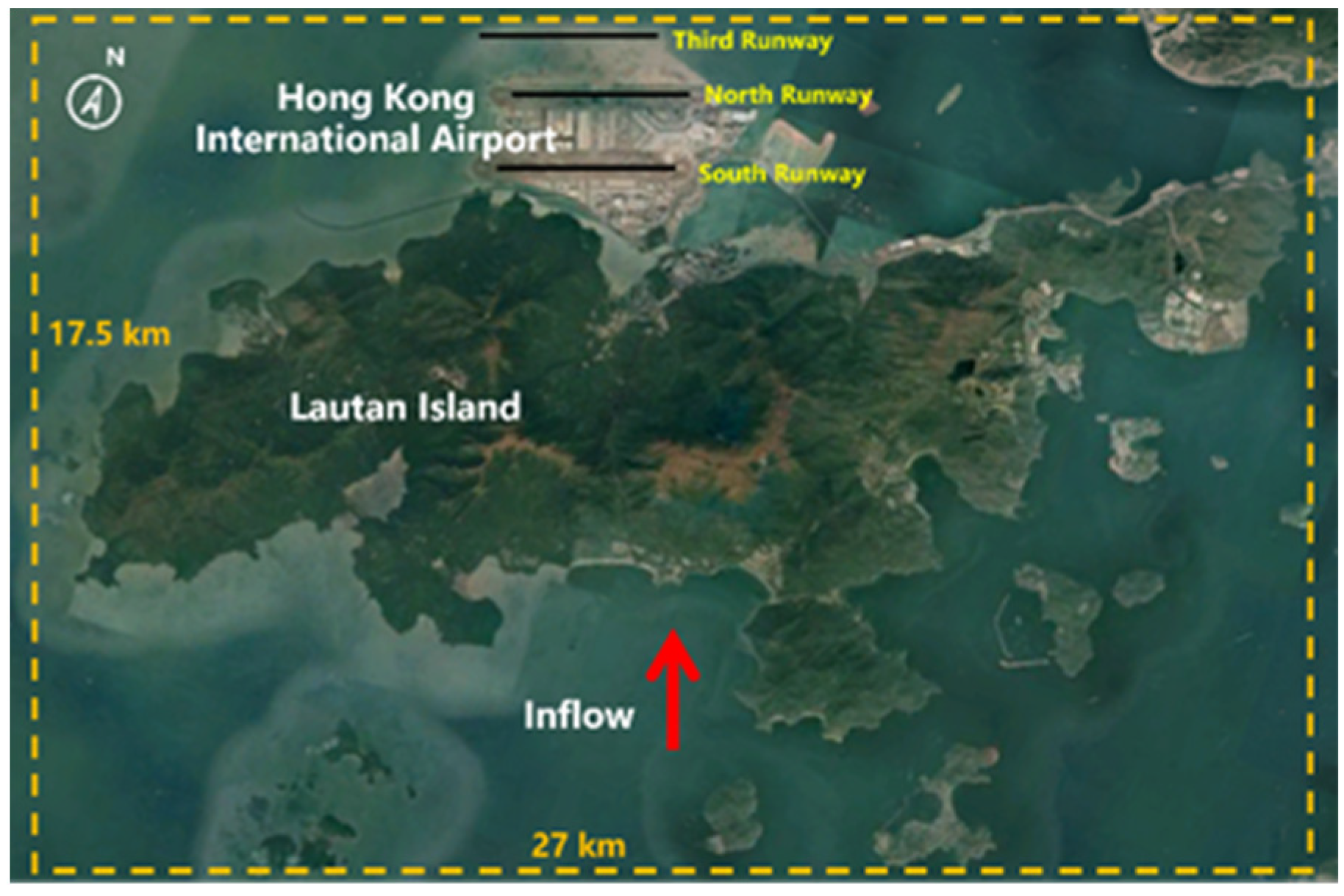
2.1. Study Location
2.2. Data Processing from Doppler LiDAR
2.3. Machine Learning Regression Algorithms
2.3.1. Light Gradient Boosting Machine (LightGBM) Regression
2.3.2. Extreme Gradient Boosting (XGBoost) Regression
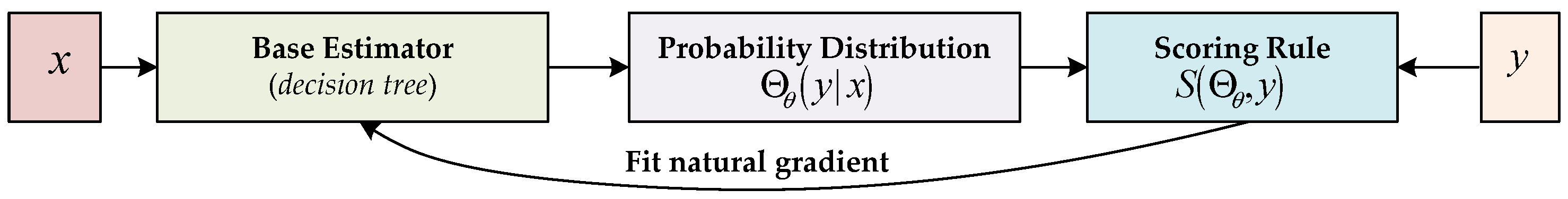
2.3.3. Natural Gradient Boosting (NGBoost) Regression
2.3.4. Categorical Boosting (CatBoost) Regression
2.3.5. Adaptive Boosting (AdaBoost) Regression
- The weight distribution is initialized as ;
- At iteration , the weak learning is trained, i.e.,, using the weight distribution;
- The weight distribution is updated in accordance with previous instances of the training dataset as ;
- The final output over all the iterations is returned as and .
2.3.6. Random Forest (RF) Regression
2.4. Principle of Bayesian Optimization
2.5. Performance Assessment
3. Results and Discussion
4. Conclusions and Recommendations
- On the testing dataset (intense wind-shear data of HKIA-based LiDAR from 1 January 2020 to 31 December 2020), the Bayesian optimized-XGBoost model had the best overall performance of all the optimized machine learning regression models, with an MAE (1.764), MSE (5.611), RMSE (2.368), and R-square (0.859), which was followed by Bayesian optimized-CatBoost model, which had an MAE (1.795), MSE (5.783), RMSE (2.404), and R-square (0.753);
- The AdaBoost regression model demonstrated the lowest performance in terms of MAE (1.863), MSE (6.815), RMSE (2.610), and R-square (0.549);
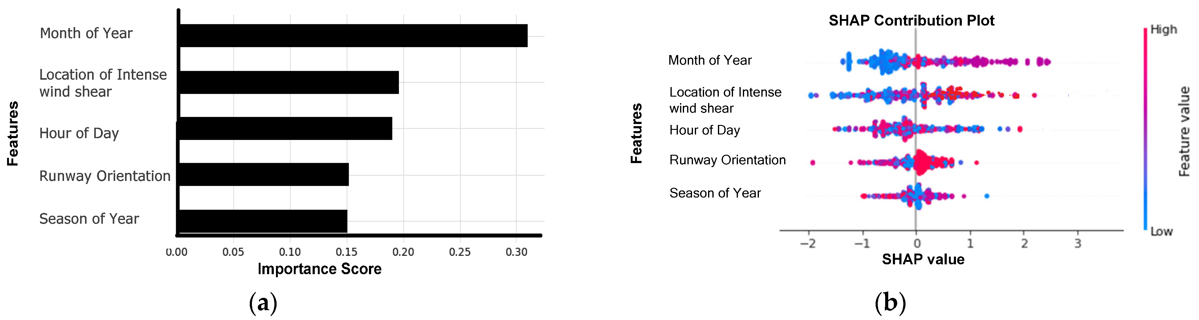
- The Bayesian optimized-XGBoost model demonstrated that the month of year was the most influential factor, followed by distance of occurrence of intense wind shear from the RWY;
- August is more likely to have intense wind-shear events. Similarly, most of the intense wind-shear events are expected to occur at RWY and 1-MD from the runway departure end. The pilots are required to be cautious during takeoff.
Author Contributions
Funding
Institutional Review Board Statement
Informed Consent Statement
Data Availability Statement
Acknowledgments
Conflicts of Interest
References
- Chan, P.W. Severe wind shear at Hong Kong International airport: Climatology and case studies. Meteorol. Appl. 2017, 3, 397–403. [Google Scholar] [CrossRef]
- Bretschneider, L.; Hankers, R.; Schönhals, S.; Heimann, J.M.; Lampert, A. Wind Shear of Low-Level Jets and Their Influence on Manned and Unmanned Fixed-Wing Aircraft during Landing Approach. Atmosphere 2021, 13, 35. [Google Scholar] [CrossRef]
- Michelson, M.; Shrader, W.; Wieler, J. Terminal Doppler weather radar. Microw. J. 1990, 33, 139. [Google Scholar]
- Shun, C.; Chan, P. Applications of an infrared Doppler lidar in detection of wind shear. J. Atmos. Ocean. Technol. 2008, 25, 637–655. [Google Scholar] [CrossRef]
- Li, L.; Shao, A.; Zhang, K.; Ding, N.; Chan, P.-W. Low-level wind shear characteristics and LiDAR-based alerting at Lanzhou Zhongchuan International Airport, China . J. Meteorol. Res. 2020, 34, 633–645. [Google Scholar] [CrossRef]
- Hon, K.-K. Predicting low-level wind shear using 200-m-resolution NWP at the Hong Kong International Airport. J. Appl. Meteorol. Climatol. 2020, 59, 193–206. [Google Scholar] [CrossRef]
- Zhang, Y.; Pan, G.; Chen, B.; Han, J.; Zhao, Y.; Zhang, C. Short-term wind speed prediction model based on GA-ANN improved by VMD. Renew. Energy 2020, 156, 1373–1388. [Google Scholar] [CrossRef]
- Zhang, Z.; Ye, L.; Qin, H.; Liu, Y.; Wang, C.; Yu, X.; Yin, X.; Li, J. Wind speed prediction method using shared weight long short-term memory network and Gaussian process regression. Appl. Energy 2019, 247, 270–284. [Google Scholar]
- Cai, H.; Jia, X.; Feng, J.; Li, W.; Hsu, Y.M.; Lee, J. Gaussian Process Regression for numerical wind speed prediction enhancement. Renew. Energy 2020, 146, 2112–2123. [Google Scholar] [CrossRef]
- Khattak, A.; Chan, P.W.; Chen, F.; Peng, H. Prediction and Interpretation of Low-Level Wind Shear Criticality Based on Its Altitude above Runway Level: Application of Bayesian Optimization–Ensemble Learning Classifiers and SHapley Additive explanations. Atmosphere 2022, 12, 2102. [Google Scholar] [CrossRef]
- Chen, F.; Peng, H.; Chan, P.W.; Ma, X.; Zeng, X. Assessing the risk of windshear occurrence at HKIA using rare-event logistic regression. Meteorol. Appl. 2020, 27, e1962. [Google Scholar] [CrossRef]
- Singh, R.K.; Rani, M.; Bhagavathula, A.S.; Sah, R.; Rodriguez-Morales, A.J.; Kalita, H.; Nanda, C.; Sharma, S.; Sharma, Y.D.; Rabaan, A.A.; et al. Prediction of the COVID-19 pandemic for the top 15 affected countries: Advanced autoregressive integrated moving average (ARIMA) model. JMIR Public Health Surveill. 2020, 6, e19115. [Google Scholar] [CrossRef] [PubMed]
- Singh, S.; Parmar, K.S.; Kumar, J.; Makkhan, S.J. Development of new hybrid model of discrete wavelet decomposition and autoregressive integrated moving average (ARIMA) models in application to one month forecast the casualties cases of COVID-19. Chaos Solitons Fractals 2020, 135, 109866. [Google Scholar] [CrossRef] [PubMed]
- Dansana, D.; Kumar, R.; Das Adhikari, J.; Mohapatra, M.; Sharma, R.; Priyadarshini, I.; Le, D.N. Global forecasting confirmed and fatal cases of COVID-19 outbreak using autoregressive integrated moving average model. Front. Public Health 2020, 8, 580327. [Google Scholar] [CrossRef] [PubMed]
- Plitnick, T.A.; Marsellos, A.E.; Tsakiri, K.G. Time series regression for forecasting flood events in Schenectady, New York. Geosciences 2018, 8, 317. [Google Scholar] [CrossRef]
- Sadeghi, B.; Ghahremanloo, M.; Mousavinezhad, S.; Lops, Y.; Pouyaei, A.; Choi, Y. Contributions of meteorology to ozone variations: Application of deep learning and the Kolmogorov-Zurbenko filter. Environ. Pollut. 2022, 310, 119863. [Google Scholar] [CrossRef]
- Smyl, S. A hybrid method of exponential smoothing and recurrent neural networks for time series forecasting. Int. J. Forecast. 2020, 36, 75–85. [Google Scholar] [CrossRef]
- Sinaga, H.; Irawati, N. A medical disposable supply demand forecasting by moving average and exponential smoothing method. In Proceedings of the 2nd Workshop on Multidisciplinary and Applications (WMA) 2018, Padang, Indonesia, 24–25 January 2018. [Google Scholar]
- Zhang, S.; Khattak, A.; Matara, C.M.; Hussain, A.; Farooq, A. Hybrid feature selection-based machine learning Classification system for the prediction of injury severity in single and multiple-vehicle accidents. PLoS ONE 2022, 17, e0262941. [Google Scholar] [CrossRef]
- Dong, S.; Khattak, A.; Ullah, I.; Zhou, J.; Hussain, A. Predicting and analyzing road traffic injury severity using boosting-based ensemble learning models with SHAPley Additive exPlanations. Int. J. Environ. Res. Public Health 2022, 19, 2925. [Google Scholar] [CrossRef]
- Khattak, A.; Almujibah, H.; Elamary, A.; Matara, C.M. Interpretable Dynamic Ensemble Selection Approach for the Prediction of Road Traffic Injury Severity: A Case Study of Pakistan’s National Highway N-5. Sustainability 2022, 14, 12340. [Google Scholar] [CrossRef]
- Goodman, S.N.; Goel, S.; Cullen, M.R. Machine learning, health disparities, and causal reasoning. Ann. Intern. Med. 2018, 169, 883–884. [Google Scholar] [CrossRef]
- Guo, R.; Fu, D.; Sollazzo, G. An ensemble learning model for asphalt pavement performance prediction based on gradient boosting decision tree. Int. J. Pavement Eng. 2022, 23, 3633–3644. [Google Scholar] [CrossRef]
- Zhao, Y.; Deng, W. Prediction in Traffic Accident Duration Based on Heterogeneous Ensemble Learning. Appl. Artif. Intell. 2022, 36, 2018643. [Google Scholar] [CrossRef]
- Freund, Y.; Schapire, R.; Abe, N. A short introduction to boosting. J. Jpn. Soc. Artif. Intell. 1999, 14, 1612. [Google Scholar]
- Ke, G.; Meng, Q.; Finley, T.; Wang, T.; Chen, W.; Ma, W.; Ye, Q.; Liu, T.Y. Lightgbm: A highly efficient gradient boosting decision tree. Adv. Neural Inf. Process. Syst. 2017, 30, 52. [Google Scholar]
- Prokhorenkova, L.; Gusev, G.; Vorobev, A.; Dorogush, A.V.; Gulin, A. CatBoost: Unbiased boosting with categorical features. Adv. Neural Inf. Process. Syst. 2018, 31. [Google Scholar]
- Chen, T.; Guestrin, C. Xgboost: A scalable tree boosting system. In Proceedings of the 22nd Acm Sigkdd International Conference on Knowledge Discovery and Data Mining, San Francisco, CA, USA, 13–17 August 2016; pp. 785–794. [Google Scholar]
- Breiman, L. Random forests. Mach. Learn. 2001, 45, 5–32. [Google Scholar] [CrossRef]
- Duan, T.; Anand, A.; Ding, D.Y.; Thai, K.K.; Basu, S.; Ng, A.; Schuler, A. Ngboost: Natural gradient boosting for probabilistic prediction. In Proceedings of the 37th International Conference on Machine Learning, Virtual Event, 13–18 July 2020; pp. 2690–2700. [Google Scholar]
- Snoek, J.; Larochelle, H.; Adams, R.P. Practical Bayesian optimization of machine learning algorithms. In Advances in Neural Information Processing Systems 25 (NIPS 2012); 2012; Volume 25, Available online: https://proceedings.neurips.cc/paper/2012/hash/05311655a15b75fab86956663e1819cd-Abstract.html (accessed on 4 August 2022).
- Chan, P.; Hon, K. Observation and numerical simulation of terrain-induced windshear at the Hong Kong International Airport in a planetary boundary layer without temperature inversions. Adv. Meteorol. 2016, 2016, 1454513. [Google Scholar] [CrossRef]
- Wu, J.; Chen, X.Y.; Zhang, H.; Xiong, L.D.; Lei, H.; Deng, S.H. Hyperparameter optimization for machine learning models based on Bayesian optimization. J. Electron. Sci. Technol. 2019, 17, 26–40. [Google Scholar]
- Victoria, A.H.; Maragatham, G. Automatic tuning of hyperparameters using Bayesian optimization. Evol. Syst. 2021, 12, 217–223. [Google Scholar] [CrossRef]
- Chan, P.W.; Hon, K.K. Observations and numerical simulations of sea breezes at Hong Kong International Airport. Weather 2022, 78, 55–63. [Google Scholar] [CrossRef]


| Date | Time | Runway | Intense Wind Shear Magnitude | Encounter Location |
|---|---|---|---|---|
| 16 May 2017 | 5:17 PM | 07RA | 35 knots | RWY |
| 19 June 2017 | 5:19 PM | 25LA | 32 knots | 1-MD |
| --- | --- | --- | --- | --- |
| --- | --- | --- | --- | --- |
| 29 March 2019 | 10:12 PM | 07CA | 37 knots | RWY |
| 29 March 2019 | 10:14 PM | 07RA | 39 knots | RWY |
| --- | --- | --- | --- | --- |
| --- | --- | --- | --- | --- |
| 21 September 2020 | 3:58 AM | 07RA | 30 knots | 2-MF |
| Dataset | Max | Median | Min | Mean | St. Dev |
|---|---|---|---|---|---|
| Entire dataset | 40 | 33 | 30 | 33.881 | 2.596 |
| Train dataset | 40 | 33 | 30 | 33.743 | 2.455 |
| Test dataset | 40 | 34 | 30 | 33.921 | 2.366 |
| Algorithm | Hyperparameters | Range | Optimal Values |
|---|---|---|---|
| LightGBM | {(n_estimators), (num_leaves), (learning rate), (reg_lambda), (reg_alpha)} | {(100–1500), (30–100), (0.001–0.2), (1.1–1.5), (1.1–1.5)} | {1180, 28, 0.10, 1.19, 1.01} |
| CatBoost | {(n_estimators), (max_depth), (learning rate)} | {(200–1500), (2–15), (0.001–0.2)} | {1060, 8, 0.08} |
| AdaBoost | {(n_estimators), (learning rate)} | {(100–1500), (0.001–0.2)} | {790, 0.04} |
| RF | {(n_estimators), (max_depth)} | {(50–1000), (2–15)} | {955, 5} |
| XGBoost | {(n_estimators), (num_leaves), (learning rate), (reg_lambda), (reg_alpha)} | {(100–1500), (30–100), (0.001–0.2), (1.1–1.5), (1.1–1.5)} | {880, 65, 0.05, 1.18, 1.40} |
| NGBoost | {(n_estimators), (learning rate)} | {(100–1500), (0.001–0.2)} | {1130, 0.03} |
| Models | Performance Metrics | |||
|---|---|---|---|---|
| MAE | MSE | RMSE | R-Square | |
| LightGBM | 1.813 | 5.840 | 2.416 | 0.711 |
| NGBoost | 1.858 | 6.298 | 2.509 | 0.619 |
| Random Forest | 1.851 | 6.194 | 2.488 | 0.647 |
| CatBoost | 1.795 | 5.783 | 2.404 | 0.753 |
| XGBoost | 1.764 | 5.611 | 2.368 | 0.859 |
| AdaBoost | 1.863 | 6.815 | 2.610 | 0.549 |
Disclaimer/Publisher’s Note: The statements, opinions and data contained in all publications are solely those of the individual author(s) and contributor(s) and not of MDPI and/or the editor(s). MDPI and/or the editor(s) disclaim responsibility for any injury to people or property resulting from any ideas, methods, instructions or products referred to in the content. |
© 2023 by the authors. Licensee MDPI, Basel, Switzerland. This article is an open access article distributed under the terms and conditions of the Creative Commons Attribution (CC BY) license (https://creativecommons.org/licenses/by/4.0/).
Share and Cite
Khattak, A.; Chan, P.-W.; Chen, F.; Peng, H. Time-Series Prediction of Intense Wind Shear Using Machine Learning Algorithms: A Case Study of Hong Kong International Airport. Atmosphere 2023, 14, 268. https://doi.org/10.3390/atmos14020268
Khattak A, Chan P-W, Chen F, Peng H. Time-Series Prediction of Intense Wind Shear Using Machine Learning Algorithms: A Case Study of Hong Kong International Airport. Atmosphere. 2023; 14(2):268. https://doi.org/10.3390/atmos14020268
Chicago/Turabian StyleKhattak, Afaq, Pak-Wai Chan, Feng Chen, and Haorong Peng. 2023. "Time-Series Prediction of Intense Wind Shear Using Machine Learning Algorithms: A Case Study of Hong Kong International Airport" Atmosphere 14, no. 2: 268. https://doi.org/10.3390/atmos14020268
APA StyleKhattak, A., Chan, P.-W., Chen, F., & Peng, H. (2023). Time-Series Prediction of Intense Wind Shear Using Machine Learning Algorithms: A Case Study of Hong Kong International Airport. Atmosphere, 14(2), 268. https://doi.org/10.3390/atmos14020268