North–South IMF Disturbance Detection via an Adaptive Filter Approach

Abstract

Geomagnetic storm-detection algorithms are important for space-weather-warning services to provide reliable warnings (e.g., ionospheric disturbances). For that reason, a new approach using an adaptive filter (least mean squares algorithm) for the detection of geomagnetic storms based on the volatility of the north–south interplanetary magnetic field $B_z$ is presented. The adaptive filter is not dependent on solar wind plasma measurements, which are more frequently affected by data gaps than $B_z$, and is less dependent on the magnitude of $B_z$ disturbances compared with other detection algorithms (e.g., static thresholds). The configuration of the filter is discussed in detail with three geomagnetic storm events, and required optimization as well as possible extensions are discussed. However, the proposed configuration performs satisfactorily without further improvements, and good correlations are observed with geomagnetic indices. Long-term changes are also reflected by the filter (solar cycles 23 and 24), and thus the performance is not affected by different solar wind conditions during the solar minimum and maximum. Conclusively, the proposed filter provides a good solution when more complex approaches (e.g., solar-wind–magnetosphere coupling functions) that rely on solar wind plasma measurements are not available.

1. Introduction

Space weather-driven variations in the ionosphere can cause significant disruptions to critical infrastructure and services [1,2]. This particularly impacts communications and navigation services, which are affected in a variety of ways by changes in the magnetosphere–ionosphere–thermosphere (MIT) system [3]. Such interactions are driven by, e.g., interplanetary coronal mass ejections (ICMEs), which cause considerable changes in the interplanetary magnetic field (IMF) and other solar wind parameters [4].

For example, the proton density and velocity increase significantly with the shock front of ICMEs, while the IMF components are affected by complex interactions. In particular, changes in the north–south IMF component are of interest in this context, since a southward directed IMF interacts more strongly with Earth’s magnetosphere [5]. For this reason, the geoeffectiveness of storms’ described solar-wind–magnetosphere coupling functions is commonly calculated from the north–south IMF component $B_z$ or the east–west IMF component $B_y$ [6,7].

Disturbances of the solar wind due to ICME are categorized into different types, including the compression region (sheath), ejecta and magnetic cloud (MC). Additionally, disturbances may be caused by co-rotating interaction regions (CIR), which dominate during the descending phase of the solar cycle [8]. These different phenomena can be identified using different solar wind measurements [9,10] and are of interest to predict geomagnetic storm conditions. For this reason, optimally, the analysis of such events is performed with a combination of different solar wind parameters to identify the different characteristics.

However, in operational applications, this is not always possible (e.g., due to data gaps), and only certain solar wind parameters may be available. The detection of disturbances in solar wind with such a restricted parameter set then requires different methods.

In the present study, the detection of $B_z$ disturbances is investigated to provide an additional solution for the solar-wind-driven ionosphere model by Schmölter and Berdermann [11]. The model predicts ionospheric disturbances (i.e., total electron content perturbations) during geomagnetic storms with real-time solar wind measurements (triggered by the detection of an event) and, thus, relies on precise storm onset time estimations. The required onset time may be calculated from defined thresholds that are applied to IMF and solar wind plasma measurements [11] or solar-wind–magnetosphere coupling functions [7].

However, both approaches are affected by data gaps in the solar wind plasma measurements. For example, a calculation of the effective solar wind pressure [7] is only possible if both the proton density and velocity are available (coverage of approximately 60% with Advanced Composition Explorer data in the investigated time period from 1998 to 2020). Furthermore, both approaches do not account for differences in the solar wind during the phases of the 11 year solar cycle (e.g., the frequency of ICME and CIR or dominance of slow and fast solar wind), and thus the performance is different during the solar minimum and maximum [11].

The adaptive filter approach investigated in the present study is designed as a backup solution for the solar-wind-driven ionosphere model by Schmölter and Berdermann [11] to continuously provide storm onset time estimations even when solar wind plasma measurements are not available. The $B_z$ measurements are stable, with only an insignificant number of data gaps for operation of the filter, which allows for continuous calculation. In addition, the different conditions depending on the 11 year solar cycle are considered, since the estimation of the storm onset does not depend on static thresholds. Instead, significant changes are identified based on the weight of the applied least mean squares (LMS) algorithm.

Generally, adaptive filters are applied to either estimate a desired time series (noise-free) or to detect changes in that time series via an optimization algorithm [12,13,14]. The applied algorithms adjust continuously, and therefore adaptive filters are sequential, nonlinear and, in some cases, nondeterministic. The group of filters is popular in different fields, e.g., economics [15,16], with an interest in establishing reliable forecast models. Adaptive filters are also applied to different space weather topics to predict phenomena or to combine different results.

Zhou and Wei [17] applied an adaptive filter approach to predict recurrent geomagnetic disturbances based on a geomagnetic index. The study specifically used the filter’s ability to adapt to the observed patterns of the recurrent geomagnetic disturbances to improve the prediction performance. Podladchikova et al. [18] applied an adaptive Kalman filter approach to improve the solar wind speed forecast based on various solar wind measurements. Ionospheric parameter were also investigated with adaptive filter approaches [19]. Thus, adaptive filters can be successfully applied in space weather research (especially in combination with other methods) and are of interest to investigate disturbances in solar wind measurements.

For implementation of the proposed adaptive filter approach, the volatility of $B_z$ is introduced, and its geomagnetic storm detection performance is analyzed and discussed (initial comparison with non-adaptive volatility but multiple time windows). The term volatility describes the deviations observed in time series and is commonly used in economic contexts, for example, as the standard deviation of logarithmic rates. In the present study, the term is used primarily to distinguish the calculated filter results from the standard deviation but also to indicate that it may be replaced with other designs in the future. The obtained parameters (e.g., the optimal time window and learning rate) are applied as appropriate inputs to the adaptive filter and, using a manually optimized configuration, the results of the filter runs are analyzed for selected geomagnetic storms.

In addition to the onset time, the intensity of the storms is also investigated to assess possible applications in future studies. Based on these analyses, required and optional extensions of the approach are discussed.

2. Data

The present study applies measurements of the north–south IMF component and geomagnetic indices (from 1998 to 2020) complementing the work in previous studies [7,11] and ensuring the comparability of the calculated performance measurements.

2.1. Measurements of the North–South IMF Component

The interplanetary magnetic field (IMF), including the north–south component $B_z$ is observed with the Magnetic Field Experiment (MAG) [20] on the board National Aeronautics and Space Administration (NASA) Advanced Composition Explorer (ACE) [21]. The 16-second averages of $B_z$ (level 2 data) in geocentric solar magnetospheric (GSM) coordinates were provided by the NASA ACE Science Center [22,23] covering solar cycles 23 and 24. Thus, a comprehensive data set for the analysis, training, and validation of geomagnetic storm forecasts is available. Additionally, the implementation of the solar-wind-driven ionosphere model for the effects of geomagnetic storms by Schmölter and Berdermann [11] utilizes ACE/MAG measurements of $B_z$, and for this reason, the analysis in the present study applies the data set as well.

2.2. Geomagnetic Indices

The present study applies Kp and Dst to investigate the storm detection performance of different approaches. For this purpose, correlation coefficients and performance measurements are calculated from the applied filters and geomagnetic indices. This approach neglects the varying correlations between solar wind and IMF measurements with geomagnetic activity (i.e., different correlations during the initial, main and recovery phases) and, thus, is not an absolute measure for the performance. Nevertheless, relative differences in the storm detection performance are well represented, thereby, allowing a ranking of the different approaches [7].

The 1 h disturbance storm time (Dst) index is a commonly used parameter to quantify the impact of geomagnetic storms. Dst describes the impact on Earth’s ring current during geomagnetic storms [24], and measurements were provided by World Data Center for Geomagnetism (WDC) in Kyoto [25,26,27]. The good correlation of the Dst index with solar wind plasma (e.g., proton density and speed) and IMF (e.g., $B_z$) features [28,29,30,31,32] qualifies this observable for the analysis of geomagnetic storm-detection algorithms.

The 3 h K indices (and the planetary Kp index) describe the disturbances in the horizontal component of Earth’s magnetic field during geomagnetic storms [33,34,35,36]. The Kp index is provided by the German Research Centre for Geosciences in Potsdam [37,38], and its good correlation with different solar wind features [39,40] qualifies this observable for the analysis of geomagnetic storm-detection algorithms. In the present study, calculations using geomagnetic indices are performed with a time resolution of 1 h. For this reason, the Kp index is linearly interpolated at the corresponding time steps.

Both geomagnetic activity indices were applied in previous studies in the scope of the forecast model for the effects of geomagnetic storms [11]. Therefore, the indices are used in the present extended analysis to ensure comparability.

3. Results

3.1. Volatility of the North–South IMF Component

For the definition of a reliable adaptive filter, the analysis of the input data and methods applied are crucial. For this reason, the north–south IMF component $B_z$ and possible candidates for the $B_z$ volatility are investigated during geomagnetic storms. Generally, the volatility ${\sigma }^{\prime }$ may be described with the standard deviation $\sigma$ according to

$${\sigma }_{t,w}=\sqrt{\frac{1}{w}\sum _{i=t-w}^t{(x_i-{\mu }_{t,w})}^2}.$$

(1)

This ${\sigma }_{t,w}$ time series is calculated from the data points $x_i$ (i.e., $B_z$) at each time step t for a time window w. Thus, changes in the volatility may be observed and used for further analyses. In the present study, the volatility ${\sigma }_{t,w}^{\prime }$ is calculated according to the root mean square (RMS) as

$${\sigma }_{t,w}^{\prime }=\sqrt{\frac{1}{w}\sum _{i=t-w}^t{\left(x_i\right)}^2}.$$

(2)

While the standard deviation accounts only for the difference to the mean ${\mu }_{t,w}$, the RMS also considers the absolute value. Therefore, $B_z$ oscillations (increased ${\sigma }_{t,w}$) as well as southward trends of $B_z$ (decreased ${\mu }_{t,w}$) during geomagnetic storms may be better represented using Equation (2). The characteristics of these changes are considered in various solar-wind-driven ionosphere models and implemented via empirical relationships [41,42] or solar-wind–magnetosphere coupling functions [7]. However, a disadvantage of such approaches is that the defined thresholds are static and, thus, depend on the observed solar activity in the training data set.

The present study investigates an adaptive approach as proposed for time series data [43]. For this purpose, an adaptive volatility filter using ${\sigma }_{t,w}^{\prime }$ is implemented, which is not dependent on the $B_z$ or $\sigma \left(B_z\right)$ thresholds. Instead, disturbance detection is performed using the observed weight of a least mean squares (LMS) algorithm, and an estimate of the geomagnetic activity is calculated using the instantaneous volatility (according to optimized w). Since the configuration of the filter is based on several steps, the difference between ${\sigma }^{\prime }\left(B_z\right)$ and $\sigma \left(B_z\right)$ is examined in more detail first.

The difference between ${\sigma }^{\prime }\left(B_z\right)$ and $\sigma \left(B_z\right)$ is shown in Figure 1 using a static time window of 2 h.

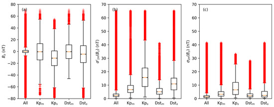
Figure 1. Box plots for north–south IMF component $B_z$ (a), volatility ${\sigma }^{\prime }\left(B_z\right)$ (b) and standard deviation $\sigma \left(B_z\right)$ (c). ${\sigma }^{\prime }\left(B_z\right)$ and $\sigma \left(B_z\right)$ are calculated for a time window of 2 h. Each panel shows the distribution for the whole data set (from 1998 to 2020) and according to moderate and severe geomagnetic storm conditions. Kp and Dst are applied to define geomagnetic storm conditions. Each box marks the interquartile range, and each vertical line marks minimum and maximum. Outliers are marked with red crosses.

The first box plot in each panel represents the whole data set from 1998 to 2020. The following box plots represent each data set for moderate and severe geomagnetic storm conditions. The selection using the Kp index considers values greater than 5 for moderate storms (Kp ${}_m$) and values greater than 8 for severe storms (Kp${}_s$). The selection using the Dst index considers values smaller than −50 nT for moderate storms (Dst${}_m$) and values smaller than −100 nT for severe storms (Dst${}_s$).

In each period defined by these conditions, all 16-second averages of $B_z$, ${\sigma }^{\prime }\left(B_z\right)$ and $\sigma \left(B_z\right)$ are selected (between start and end of each geomagnetic storm). The southward trend of $B_z$ during geomagnetic storms is reflected in Figure 1a; however, a significant decrease of the median (as well as lower and upper quartile) occurs only for Kp ${}_s$. ${\sigma }^{\prime }\left(B_z\right)$ and $\sigma \left(B_z\right)$ in Figure 1b,c are significantly increased for moderate and severe storms; however, the distinctions between different conditions are more strongly pronounced for ${\sigma }^{\prime }\left(B_z\right)$.

The correlation and performance (prediction of geomagnetic activity) are further analyzed via the approach applied in preceding studies [7]. First, binary time series (0 = no storm and 1 = storm) are calculated from ${\sigma }^{\prime }\left(B_z\right)$ and $\sigma \left(B_z\right)$ for time windows from 1 to 48 h and for various thresholds covering the entire range of values (resulting in a matrix for each data set). A similar binary time series is calculated from the geomagnetic indices using the introduced thresholds for moderate and severe storms (see Figure 1).

The results based on ${\sigma }^{\prime }\left(B_z\right)$ and $\sigma \left(B_z\right)$ are then compared with the observed conditions based on geomagnetic indices, and the confusion matrix for each threshold and time window w is calculated. From these, in turn, the hit rate (POD) and false-alarm rate (POFD) are determined. Both POD and POFD are combined in a receiver operating characteristic (ROC) plot reflecting the performance for each configuration. Additionally, the optimal performance is presented using the true skill statistic (TSS = POD − POFD), where the highest value is identified at the maximum distance from the ROC center line.

The ROC plot in Figure 2 shows the results for different ${\sigma }^{\prime }\left(B_z\right)$ configurations and the most optimal $\sigma \left(B_z\right)$ configuration.

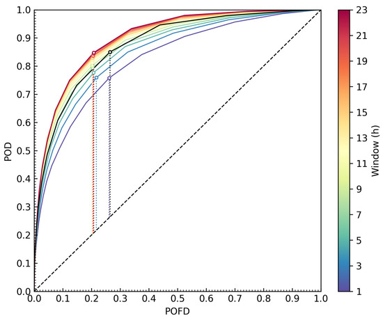
Figure 2. The ROC curves of ${\sigma }^{\prime }\left(B_z\right)$ for different windows (color coded) and the optimal $\sigma \left(B_z\right)$ configuration (black, window of 3 h) are shown. The optimal value for each parameter according to the true skill statistic is marked with corresponding circles and dotted lines. The no-skill condition is marked with a black dashed line.

The maximum TSS of ${\sigma }^{\prime }\left(B_z\right)$ configurations increases (w smaller than 23 h) and generally ${\sigma }_w^{\prime }\left(B_z\right)$ performs better than corresponding ${\sigma }_w\left(B_z\right)$. Additionally, there are several ${\sigma }^{\prime }\left(B_z\right)$ configurations with smaller time windows but greater maximum TSS than the $\sigma \left(B_z\right)$ configuration with the highest maximum TSS (window of 3 h). Thus, ${\sigma }^{\prime }\left(B_z\right)$ according to Equation (2) is the preferred input data set for the adaptive filter. The POD for different ${\sigma }^{\prime }\left(B_z\right)$ configurations at a limited POFD of 10% is shown in Figure 3. This applied limit for the POFD is required because the configurations obtained using the maximum TSS have POFDs that are not acceptable for an operational framework.

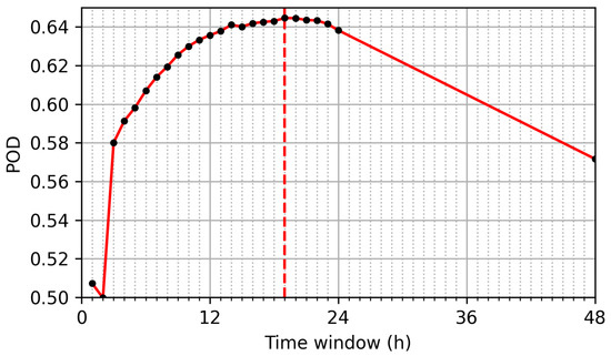
Figure 3. The hit rate (POD) for ${\sigma }^{\prime }\left(B_z\right)$ configurations with different time windows (black dots and red line). The dashed red line marks the maximum POD at 19 h. The false-alarm rate (POFD) is limited to 10%.

The maximum POD is observed at a time window of 19 h (4275 samples), and therefore this configuration is selected for the initial setup of the desired ${\sigma }_d^{\prime }\left(B_z\right)$ filter. Additionally, a fast ${\sigma }_f^{\prime }\left(B_z\right)$ and slow ${\sigma }_s^{\prime }\left(B_z\right)$ filter are required for the further analysis. The windows of these filters are set to arbitrary values of 1 and 24 h. Thus, the three windows of the fast, desired and slow filter are related according to

$$w_f<w_d<w_s.$$

(3)

The estimated configuration ${\sigma }_d^{\prime }\left(B_z\right)$ with optimized w may be applied for the detection of $B_z$ disturbances without further adjustment. However, this approach would rely on the applied training data and, e.g., may perform differently throughout the solar cycle. These variations are accounted by the adaptive filter approach, which is implemented using the three estimated filters.

3.2. Detection of Changes in the North–South IMF Component

The detection of changes in the the north–south IMF component $B_z$ is implemented using an adaptive filter that calculates the instantaneous volatility ${\sigma }_{t,o}^{\prime }\left(B_z\right)$ at each time step t according to

$${\sigma }_{t,o}^{\prime }={\lambda }_t{\sigma }_{t,f}^{\prime }+(1-{\lambda }_t){\sigma }_{t,s}^{\prime }.$$

(4)

The weight ${\lambda }_t$ that is applied to the fast ${\sigma }_f^{\prime }\left(B_z\right)$ and slow ${\sigma }_s^{\prime }\left(B_z\right)$ filter is adjusted at each time step t as well. For this purpose, the difference between the filters and the corresponding gradients (one-sided difference of second order) are optimized using a least mean squares (LMS) algorithm as

$${\lambda }_{t+1}={\lambda }_t+({\sigma }_{t,f}^{\prime }-{\sigma }_{t,s}^{\prime })·({\sigma }_{t,d}^{\prime }-{\sigma }_{t,o}^{\prime })·l_1+(d{\sigma }_{t,f}^{\prime }-d{\sigma }_{t,s}^{\prime })·(d{\sigma }_{t,d}^{\prime }-d{\sigma }_{t,o}^{\prime })·l_2.$$

(5)

The learning rate is separated into $l_1$ and $l_2$, which control the impact of ${\sigma }^{\prime }\left(B_z\right)$ and $d{\sigma }^{\prime }\left(B_z\right)$ on changes of $\lambda$. The mean impact of the ${\sigma }_f^{\prime }\left(B_z\right)$- and ${\sigma }_s^{\prime }\left(B_z\right)$-related terms on $\lambda$ are estimated according to

$${\sigma }_f^{\prime }-{\sigma }_s^{\prime }\sim -0.28\mathrm{nT}$$

(6)

and

$$d{\sigma }_f^{\prime }-d{\sigma }_s^{\prime }\sim 0\mathrm{nT}.$$

(7)

Thus, $\lambda$ converges generally towards small values favoring the desired ${\sigma }_d^{\prime }\left(B_z\right)$ and slow ${\sigma }_s^{\prime }\left(B_z\right)$ filter. Both terms increase strongly during significant $B_z$ variations, and then $\lambda$ increases favoring the fast ${\sigma }_f^{\prime }\left(B_z\right)$ filter. A change is detected if $\lambda$ is greater than the threshold $\gamma$, which is set to 0.99 for the filter configuration. The detection triggers a decrease of $l_1$ for a period of $1.2·w_s$, which prevents strong fluctuations of $\lambda$. For this purpose, a simple polynomial function of any order k may be applied to scale $l_1$ according to

$$l_1^{\prime }=l_1{\left(\frac{t-t_0}{1.2·w_s}\right)}^k.$$

(8)

Since the change from disturbed to undisturbed $B_z$ has to be identified as well, another selection is added, which requires ${\sigma }_o^{\prime }\left(B_z\right)$ to be greater than the mean ${\sigma }_d^{\prime }\left(B_z\right)$ before the change detection. The mean of ${\sigma }_d^{\prime }\left(B_z\right)$ is calculated with the end time $t_E$ of the preceding detection according to

$$\overline{{\sigma }_{t,d}^{\prime }\left(B_z\right)}=\frac{1}{\left|\right\{t_E...t\left\}\right|}\sum _{i=t_E}^t{\sigma }_{i,d}^{\prime }\left(B_z\right).$$

(9)

The filter configuration based on the introduced parameters for the further analysis is summarized in Table 1.

Table 1. Adaptive filter configuration.

Parameter	Variable	Value
Fast filter window	$w_f$	1 h
Slow filter window	$w_s$	24 h
Desired filter window	$w_d$	19 h
Initial weight	${\lambda }_0$	0.01
Filter learning rate	$l_1$	0.025
Gradient learning rate	$l_2$	1
Threshold	$\gamma$	0.99

Since the initial weight ${\lambda }_0$ is only an estimate, a training period of $w_s$ is performed prior to each of the example runs. Thus, stable initial conditions for $\lambda$ and ${\sigma }_o^{\prime }\left(B_z\right)$ converge at the start of the investigated storm events. The estimated onset times are then compared to the time of the associated geomagnetic storm sudden commencement from the ICME catalog by Richardson and Cane [44], which is continuously updated and revised [45,46].

The first example run is performed for a geomagnetic storm event in April 2000. The observed storm during this period is reflected with a strong decrease of $B_z$ from 6 April 2000 16:00 until 6 April 2000 23:00 (see Figure 4a). Strong $B_z$ fluctuations are observed in the following period from 7 April 2000 00:00 until 7 April 2000 08:00.

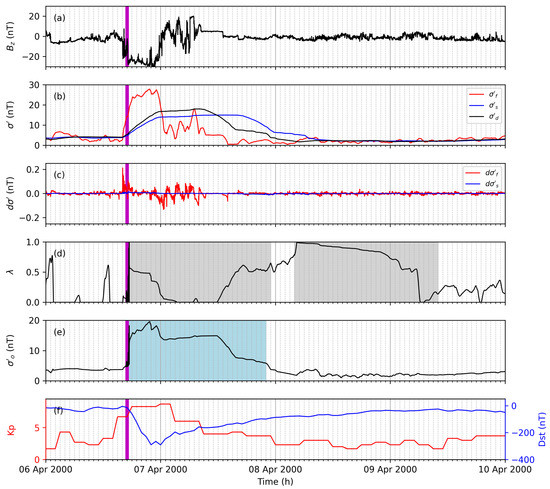
Figure 4. The north–south IMF component $B_z$ (a), volatility ${\sigma }^{\prime }$ (b), gradient of the volatility $d{\sigma }^{\prime }$ (c), weight $\lambda$ (d), instantaneous volatility ${\sigma }_o^{\prime }$ (e), and Kp and Dst (f) are shown for a geomagnetic storm starting 6 April 2000. ${\sigma }^{\prime }$ and $d{\sigma }^{\prime }$ are presented for the slow (blue) and fast (red) volatility filter. The ${\sigma }^{\prime }$ of the desired volatility filter (b) is shown with the black line. The blue-shaded area marks the disturbed period according to the adaptive filter. The gray-shaded area marks periods with scaled learning rates. The time of the associated geomagnetic storm sudden commencement is marked with a vertical magenta line.

The slow volatility ${\sigma }_s^{\prime }\left(B_z\right)$ filter (blue line in Figure 4b) reflects a stable estimate for the $B_z$ changes and the fast volatility ${\sigma }_f^{\prime }\left(B_z\right)$ filter (red line in Figure 4b) describes the immediate $B_z$ changes well (e.g., strong $B_z$ decrease during storm onset). These immediate changes are even more strongly pronounced with the gradient $d{\sigma }_f^{\prime }\left(B_z\right)$ (red line in Figure 4c). The instantaneous volatility ${\sigma }_o^{\prime }\left(B_z\right)$ calculated from the proposed adaptive filter shows the desired storm detection (see Figure 4e). A significant ${\sigma }_o^{\prime }\left(B_z\right)$ increase is observed during the storm onset time, and the maximum enhancement occurs during the strong decrease of $B_z$.

During the period of strong $B_z$ fluctuations, ${\sigma }_o^{\prime }\left(B_z\right)$ decreases but a stable estimate is observed. Thus, ${\sigma }_o^{\prime }\left(B_z\right)$ shows an immediate response to significant $B_z$ changes and estimates a stable volatility for different $B_z$ variations (on different time scales). Additionally, the enhanced geomagnetic activity is estimated similar to other coupling functions [7]. The crucial difference, however, is that no ${\sigma }_o^{\prime }\left(B_z\right)$ threshold is applied to define the storm onset time (e.g., requiring ${\sigma }_o^{\prime }\left(B_z\right)$ to be greater than 10 nT).

The second example run was performed for a geomagnetic storm event in March 2015. The observed storm during this period is reflected with a strong increase and immediate decrease of $B_z$ from 17 March 2015 04:00 until 17 March 2015 06:00 (see Figure 5a).

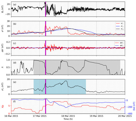
Figure 5. The north–south IMF component $B_z$ (a), volatility ${\sigma }^{\prime }$ (b), gradient of the volatility $d{\sigma }^{\prime }$ (c), weight $\lambda$ (d), instantaneous volatility ${\sigma }_o^{\prime }$ (e), and Kp and Dst (f) are shown for a geomagnetic storm starting 17 March 2015. ${\sigma }^{\prime }$ and $d{\sigma }^{\prime }$ are presented for the slow (blue) and fast (red) volatility filter. The ${\sigma }^{\prime }$ of the desired volatility filter (b) is shown with the black line. The blue-shaded area marks the disturbed period according to the adaptive filter. The gray-shaded area marks periods with scaled learning rates. The time of the associated geomagnetic storm sudden commencement is marked with a vertical magenta line.

Strong $B_z$ decreases and fluctuations are observed in the following period from 17 March 2015 07:00 until 18 March 2015 00:00. Moderate $B_z$ fluctuations are still observed after this period. Additionally, $B_z$ decreases are observed during 16 March 2015 23:00 and 17 March 2015 02:00. The adaptive filter reflects these variations well but the storm onset time is detected too early due to preceding $B_z$ decreases (see Figure 5e). This example run demonstrates how the proposed adaptive filter is able to identify geomagnetic storms independent of strong ${\sigma }_o^{\prime }\left(B_z\right)$ increases; however, on the other hand, the applied configuration is too sensitive, and a slower learning rate may be more appropriate.

The third example run is performed for a geomagnetic storm event in October and November 2003 (the Halloween storm), which is characterized by two strong shocks, extremely high solar wind speeds, comparatively less strong IMF variations and a strong impact on Earth [47]. Strong $B_z$ fluctuations are observed for the first shock with a minimum of −50 nT from 29 October 2003 06:00 until 29 October 2003 11:00, and a $B_z$ decrease is observed from 29 October 2003 18:00 until 30 October 2003 03:00 (see Figure 6a). $B_z$ fluctuations are observed for the second shock from 30 October 2003 17:00 until 31 October 2003 03:00.

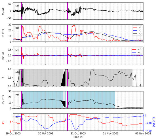
Figure 6. The north–south IMF component $B_z$ (a), volatility ${\sigma }^{\prime }$ (b), gradient of the volatility $d{\sigma }^{\prime }$ (c), weight $\lambda$ (d), instantaneous volatility ${\sigma }_o^{\prime }$ (e), and Kp and Dst (f) are shown for a geomagnetic storm starting 29 October 2003. ${\sigma }^{\prime }$ and $d{\sigma }^{\prime }$ are presented for the slow (blue) and fast (red) volatility filter. The ${\sigma }^{\prime }$ of the desired volatility filter (b) is shown with the black line. The blue-shaded area marks the disturbed period according to the adaptive filter. The gray-shaded area marks periods with scaled learning rates. The time of the associated geomagnetic storm sudden commencement is marked with a vertical magenta line.

The adaptive filter identifies the two storm periods well and an immediate response during the storm onset is observed (see Figure 6e). However, strong ${\sigma }_o^{\prime }\left(B_z\right)$ fluctuations are observed during the end of the first storm period due to overestimated $\lambda$ adjustments. The adaptive filter is not stable during this period, and the following period could be influenced due to these undesired variations (e.g., due to a false storm detection). Nevertheless, the adaptive filter also represents this geomagnetic storm with two shocks well considering that the configuration (see Table 1) is not optimized.

Figure 4, Figure 5 and Figure 6 present ICME-driven geomagnetic storms. Figure 7, on the other hand, shows an example for CIR-driven $B_z$ disturbances.

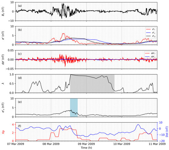
Figure 7. The north–south IMF component $B_z$ (a), volatility ${\sigma }^{\prime }$ (b), gradient of the volatility $d{\sigma }^{\prime }$ (c), weight $\lambda$ (d), instantaneous volatility ${\sigma }_o^{\prime }$ (e), and Kp and Dst (f) are shown for CIR-driven geomagnetic activity. ${\sigma }^{\prime }$ and $d{\sigma }^{\prime }$ are presented for the slow (blue) and fast (red) volatility filter. The ${\sigma }^{\prime }$ of the desired volatility filter (b) is shown with the black line. The blue-shaded area marks the disturbed period according to the adaptive filter. The gray-shaded area marks periods with scaled learning rates.

The selected event is during the solar minimum, and thus low geomagnetic activity is observed. The CIR starting 7 March 2009 22:00 [9] causes less-pronounced $B_z$ variations than does the discussed ICME-driven geomagnetic storms. The interplanetary shock was reported at 8 March 2009 17:00 [9], and a corresponding Dst decrease is observed (see Figure 7f). The adaptive filter reflects the observed geomagnetic activity partially for both geomagnetic indices. ${\sigma }_o^{\prime }\left(B_z\right)$ correlates well with Kp; however, the estimated onset time is too late for the observed increase. However, the Dst decrease is well represented with the estimated onset time. Thus, this example shows that the adaptive filter is able to detect less-pronounced $B_z$ disturbances.

4. Discussion

The ${\sigma }_o^{\prime }\left(B_z\right)$ performance is not significantly changed compared to the ${\sigma }_d^{\prime }\left(B_z\right)$ performance (see Figure 2 and Figure 3) according to POD ($-1.70\%$) and POFD ($-3.70\%$). This can be attributed to the precise estimation of the storm onset time being less relevant to the performance compared to storm duration, and the presence of geomagnetic storms in only a fraction of the data set ($4.53\%$). The investigated ICME-driven geomagnetic storms (see Figure 4, Figure 5 and Figure 6) and CIR-driven geomagnetic activity (see Figure 7) are well represented by the adaptive filter approach. A general overview is calculated for an extended period from 2000 to 2020. The adaptive filter approach was executed in one continuous run, and then 1 h averages of $B_z$, ${\sigma }_d^{\prime }\left(B_z\right)$ and ${\sigma }_o^{\prime }\left(B_z\right)$ were applied to calculate annual Pearson correlation coefficients with Kp and Dst. The resulting correlation time series are shown in Figure 8.

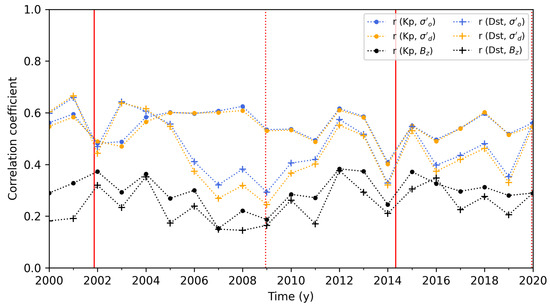
Figure 8. The annual correlation of Kp (dot) and Dst (cross) with north–south IMF component $B_z$ (black), desired volatility ${\sigma }_d^{\prime }$ (yellow) and instantaneous volatility ${\sigma }_o^{\prime }$ (blue) from 2000 to 2020. The Pearson correlation coefficient was calculated for each combination with 1 h data. The solar maxima (solid red line) and minima (dotted red line) are shown for solar cycles 23 and 24.

The annual correlation of ${\sigma }_o^{\prime }\left(B_z\right)$ (blue lines) is slightly improved compared to ${\sigma }_d^{\prime }\left(B_z\right)$ (yellow lines) but significant improvements are observed compared to $B_z$ (black lines). Regardless of whether $B_z$, ${\sigma }_d^{\prime }\left(B_z\right)$, or ${\sigma }_o^{\prime }\left(B_z\right)$ are used, Kp is generally better correlated than Dst (except for the solar maximum of solar cycle 23). In particular, during the solar minimum from 2005 to 2011, Kp is significantly better correlated than Dst, which may be related to the observed difference in Figure 7 (the solar minimum is dominated by CIR).

The interplanetary drivers significantly affect the response of Kp and Dst during geomagnetic storms [10,48], and additionally both indices are driven by different magnetospheric processes [49]. Since Kp is significantly driven by high-latitude auroral electrojets [49] and Dst is reflecting the ring current intensity [49], a different correlation with solar wind measurements is expected. For these reasons, future studies should investigate in greater detail how these characteristic may be included in the proposed adaptive filter. The different time resolutions (and interpolations of Kp) may affect the results as well.

The proposed adaptive filter with an initial configuration is able to detect $B_z$ disturbances and estimates a stable volatility during these events. For this reason, the instantaneous volatility ${\sigma }_o^{\prime }\left(B_z\right)$ may also be used to estimate geomagnetic activity if an optimized configuration is applied.

4.1. Storm Impact via Volatility

Figure 9 presents the correlation of Kp with $B_z$, ${\sigma }_d^{\prime }\left(B_z\right)$ and ${\sigma }_o^{\prime }\left(B_z\right)$ for the example runs (see Figure 4, Figure 5 and Figure 6).

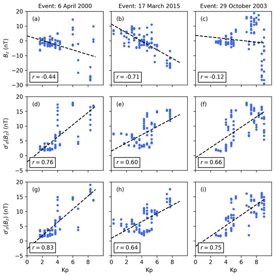
Figure 9. Scatter plots for geomagnetic storms starting 6 April 2000 (a,d,g), 17 March 2015 (b,e,h) and 29 October 2003 (c,f,i) showing the correlation of the geomagnetic index Kp with the north–south IMF component $B_z$ (a–c), desired volatility ${\sigma }_d^{\prime }$ (d–f) and instantaneous volatility ${\sigma }_o^{\prime }$ (g–i). The correlation coefficient r and trend line (black dashed line) are annotated in each plot. The data are presented in hourly resolution.

The inverse correlation of Kp and $B_z$ varies between weak and strong for the three geomagnetic storms. These differences may be accounted for by solar-wind–magnetosphere coupling functions that calculate the energy transfer from the solar wind into the magnetosphere [6]. However, this storm impact may also be calculated using ${\sigma }_o^{\prime }\left(B_z\right)$, which is well correlated with Kp for the three geomagnetic storms. In particular, the correlations for the events starting 6 April 2000 and 29 October 2003 are significantly increased. The comparison of the ${\sigma }_d^{\prime }\left(B_z\right)$ and ${\sigma }_o^{\prime }\left(B_z\right)$ correlations further shows a significant improvement due to the adaptive filter approach (approximately 10%). Thus, future studies could investigate whether an optimization of ${\sigma }_o^{\prime }\left(B_z\right)$ in regard to storm period and impact is possible. Figure 10 presents the correlation of Dst with $B_z$, ${\sigma }_d^{\prime }\left(B_z\right)$ and ${\sigma }_o^{\prime }\left(B_z\right)$ for the example runs (see Figure 4, Figure 5 and Figure 6).

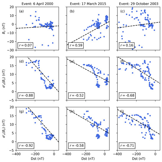
Figure 10. Scatter plots for geomagnetic storms starting 6 April 2000 (a,d,g), 17 March 2015 (b,e,h) and 29 October 2003 (c,f,i) showing the correlation of the geomagnetic index Dst with the north–south IMF component $B_z$ (a–c), desired volatility ${\sigma }_d^{\prime }$ (d–f) and instantaneous volatility ${\sigma }_o^{\prime }$ (g–i). The correlation coefficient r and trend line (black dashed line) are annotated in each plot. The data are presented in hourly resolution.

The results confirm the discussed advantages of the adaptive filter according to Kp (see Figure 9), and the comparison of the ${\sigma }_d^{\prime }\left(B_z\right)$ and ${\sigma }_o^{\prime }\left(B_z\right)$ correlations shows a significant improvement again (approximately 7%).

The long-term correlation of the adaptive filter with Kp and Dst may be considered as well (see Figure 8), since such analysis allows for the comparison of differences of geomagnetic activity during solar minima and maxima. The applied filter configuration shows an improved correlation with Kp during the solar minimum (no decrease compared to the solar maximum). Thus, changes are successfully detected even during weaker solar activity.

Including the one-sided difference in the filter algorithm (see Equation (5)) compared to other approaches [43] causes a more immediate response of the filter during significant decrease of $B_z$. Such changes are reflected differently by Kp and Dst, and other dependencies (e.g., time of year) further modify the resulting impact of the geomagnetic storm. Thus, the approach presented in this study is not able to replace solar-wind–magnetosphere coupling functions; however, an estimate of the impact is still possible.

4.2. Optimization and Extension of the Adaptive Filter Approach

The proposed adaptive filter was not optimized in the present study; however, a good detection of $B_z$ disturbances as well as a good correlation with Kp and Dst was observed. Nevertheless, an optimization should be performed in future studies, including all available historical storm events. The approach by Schmölter and Berdermann [7] that optimized a different geomagnetic storm-detection algorithm (with the data of two solar cycles) could also be applied here.

However, such an extensive optimization is expected to require long processing times for the proposed adaptive filter since the algorithm is sequential. Additionally, there are six parameters that should be considered for optimization, including $w_f$, $w_s$, $w_d$, $l_1$, $l_2$ and $\gamma$. A large number of test runs is therefore required even if only a limited set of possible values is assumed for each parameter. Adjustments to the algorithm itself (e.g., not taking gradients into account) could also be considered.

The proposed adaptive filter may also be improved with various extensions. For example, the time windows are restricted to values from 1 to 24 h, although values at higher resolution could be applied. In particular, shorter $w_f$ should be investigated (more immediate response to $B_z$ disturbances). Furthermore, weight coefficients could be applied to the selected samples (proposed filter with equal weights). For this purpose, the IMF disturbances during geomagnetic storms have to be defined more precisely and, if necessary, be categorized. However, this introduces further complexity to an automatized optimization.

The propagation delay between $B_z$ disturbances at L1 and Earth has been neglected in the present investigation but no significant impact on the qualitative comparison of calculated correlations (see Figure 9 and Figure 10) is expected. Nevertheless, this propagation delay has to be considered for the prediction of geomagnetic indices and ionosphere models. If solar wind plasma measurements are available, this delay may be calculated and added using appropriate algorithms [50,51].

The presented approach could also be applied to further IMF components or solar wind plasma measurements if the geomagnetic storm-detection capabilities are better than other approaches. However, this would require a solution for data gaps, which are more frequent for solar wind plasma measurements compared to $B_z$ measurements. For example, the filter could be restarted after each significant data gap (and the time period could be flagged accordingly); however, the implementation and optimization of such a solution would be less appropriate in the context of the solar-wind-driven ionosphere model proposed by Schmölter and Berdermann [11] with respect to the processing time.

In summary, the adaptive filter should be applied as suggested when solar wind plasma measurements are not available, and thus geomagnetic storm detection has to be performed using IMF components only. Future studies should aim to optimize the configuration in respect to the onset time, and the geomagnetic activity may be considered as well.

5. Conclusions

The adaptive filter approach introduced in the present study allows for the detection of $B_z$ disturbances and geomagnetic storms when solar wind plasma measurements—and hence solar-wind–magnetosphere coupling functions—are not available. Identifying geomagnetic storms with the proposed algorithm (see Equations (2), (4) and (5)) was less dependent on the magnitude of $B_z$ disturbances and, therefore, had better correlations with Kp and Dst (see Figure 8) compared with the $B_z$ volatility with a constant time window (or $B_z$ measurements). Thus, for example, variations due to the 11 year solar cycle were also considered (see Figure 8).

The analyses with an initial configuration (see Table 1) for selected geomagnetic storms showed satisfactory results (see Figure 4, Figure 5 and Figure 6), and the instantaneous volatility was well correlated with geomagnetic indices (see Figure 9 and Figure 10). Furthermore, the fast and slow filters provided good solutions (see Figure 2), and thus the performance was sufficient even under the worst-case conditions.

Future optimization and extension of the adaptive filter are challenging due to the sequential algorithm and the resulting processing times. For this reason, the approach should first be optimized with respect to the onset time of $B_z$ disturbances, and further changes (e.g., correlation with the geomagnetic activity) are optional. With these adjustments made, the adaptive filter could then be applied to the solar-wind-driven ionosphere model by Schmölter and Berdermann [11] or may be provided as a standalone space-weather-warning index.

References

- Baker, D.N.; Daly, E.; Daglis, I.; Kappenman, J.G.; Panasyuk, M. Effects of Space Weather on Technology Infrastructure. Space Weather 2004, 2, 2. [Google Scholar] [CrossRef]
- Eastwood, J.P.; Biffis, E.; Hapgood, M.A.; Green, L.; Bisi, M.M.; Bentley, R.D.; Wicks, R.; McKinnell, L.A.; Gibbs, M.; Burnett, C. The Economic Impact of Space Weather: Where Do We Stand? Risk Anal. 2017, 37, 206–218. [Google Scholar] [CrossRef] [PubMed]
- Sreeja, V. Impact and mitigation of space weather effects on GNSS receiver performance. Geosci. Lett. 2016, 3, 24. [Google Scholar] [CrossRef]
- Milan, S.E.; Clausen, L.B.N.; Coxon, J.C.; Carter, J.A.; Walach, M.T.; Laundal, K.; ∅stgaard, N.; Tenfjord, P.; Reistad, J.; Snekvik, K.; et al. Overview of Solar Wind-Magnetosphere-Ionosphere-Atmosphere Coupling and the Generation of Magnetospheric Currents. Space Sci. Rev. 2017, 206, 547–573. [Google Scholar] [CrossRef]
- Choi, K.E.; Lee, D.Y.; Choi, K.C.; Kim, J. Statistical properties and geoeffectiveness of southward interplanetary magnetic field with emphasis on weakly southward Bz events. J. Geophys. Res. Space Phys. 2017, 122, 4921–4934. [Google Scholar] [CrossRef]
- Gonzalez, W.D. A unified view of solar wind-magnetosphere coupling functions. Planet. Space Sci. 1990, 38, 627–632. [Google Scholar] [CrossRef]
- Schmölter, E.; Berdermann, J. Real-Time Solar Storm Onset Determination at Lagrange Point 1 (L1) Based on an Optimized Effective Pressure Parameter. URSI Radio Sci. Lett. 2021, 3. [Google Scholar] [CrossRef]
- Zhang, J.; Temmer, M.; Gopalswamy, N.; Malandraki, O.; Nitta, N.V.; Patsourakos, S.; Shen, F.; Vršnak, B.; Wang, Y.; Webb, D.; et al. Earth-affecting solar transients: A review of progresses in solar cycle 24. Prog. Earth Planet. Sci. 2021, 8, 56. [Google Scholar] [CrossRef]
- Yermolaev, Y.I.; Nikolaeva, N.S.; Lodkina, I.G.; Yermolaev, M.Y. Catalog of large-scale solar wind phenomena during 1976–2000. Cosm. Res. 2009, 47, 81–94. [Google Scholar] [CrossRef]
- Yermolaev, Y.I.; Lodkina, I.G.; Dremukhina, L.A.; Yermolaev, M.Y.; Khokhlachev, A.A. What Solar–Terrestrial Link Researchers Should Know about Interplanetary Drivers. Universe 2021, 7, 138. [Google Scholar] [CrossRef]
- Schmölter, E.; Berdermann, J. Predicting the Effects of Solar Storms on the Ionosphere Based on a Comparison of Real-Time Solar Wind Data with the Best-Fitting Historical Storm Event. Atmosphere 2021, 12, 1684. [Google Scholar] [CrossRef]
- Widrow, B. Adaptive Filters; Holt, Rinehart and Winston: New York City, NY, USA, 1971. [Google Scholar]
- Ferrara, E.; Widrow, B. The time-sequenced adaptive filter. IEEE Trans. Acoust. Speech Signal Process. 1981, 29, 679–683. [Google Scholar] [CrossRef]
- Borouje, F. Adaptive Filters: Theory and Applications, 2nd ed.; Wiley: Hoboken, NJ, USA, 2013. [Google Scholar]
- Bedendo, M.; Hodges, S.D. The dynamics of the volatility skew: A Kalman filter approach. J. Bank. Financ. 2009, 33, 1156–1165. [Google Scholar] [CrossRef]
- Catania, L.; Grassi, S.; Ravazzolo, F. Predicting the Volatility of Cryptocurrency Time-Series. In Mathematical and Statistical Methods for Actuarial Sciences and Finance; Springer International Publishing: Switzerland, Basel, 2018; pp. 203–207. [Google Scholar] [CrossRef]
- Zhou, X.Y.; Wei, F.S. Prediction of recurrent geomagnetic disturbances by using adaptive filtering. Earth Planets Space 1998, 50, 839–845. [Google Scholar] [CrossRef]
- Podladchikova, T.; Veronig, A.M.; Temmer, M.; Hofmeister, S. Solar Wind Forecast based on Data Assimilation with an Adaptive Kalman Filter. In Proceedings of the EGU General Assembly Conference Abstracts, Vienna, Austria, 8–13 April 2018; p. 8685. [Google Scholar]
- Wang, J.; Feng, F.; Ma, J. An Adaptive Forecasting Method for Ionospheric Critical Frequency of F2 Layer. Radio Sci. 2020, 55, 1–12. [Google Scholar] [CrossRef]
- Smith, C.W.; L-Heureux, J.; Ness, N.F.; Acuña, M.H.; Burlaga, L.F.; Scheifele, J. The ACE Magnetic Fields Experiment. Space Sci. Rev. 1998, 86, 613–632. [Google Scholar] [CrossRef]
- Stone, E.C.; Frandsen, A.M.; Mewaldt, R.A.; Christian, E.R.; Margolies, D.; Ormes, J.F.; Snow, F. The Advanced Composition Explorer. Space Sci. Rev. 1998, 86, 1–22. [Google Scholar] [CrossRef]
- Garrard, T.L.; Davis, A.J.; Hammond, J.S.; Sears, S.R. The ACE Science Center. Space Sci. Rev. 1998, 86, 649–663. [Google Scholar] [CrossRef]
- ASC. ACE Level 2 (Verified) Data. 2022. Available online: http://www.srl.caltech.edu/ACE/ASC/level2/index.html (accessed on 29 April 2022).
- Mayaud, P.N. Derivation, Meaning, and Use of Geomagnetic Indices; American Geophysical Union: Washington, DC, USA, 1980. [Google Scholar] [CrossRef]
- Sugiura, M.; Kamei, T. IAGA Bull. 40. 1991. Available online: http://isgi.unistra.fr/indices_dst.php (accessed on 29 April 2022).
- Nose, M.; Sugiura, M.; Kamei, T.; Iyemori, T.; Koyama, Y. Dst Index. 2015. Available online: https://doi.org/10.17593/14515-74000 (accessed on 29 April 2022). [CrossRef]
- WDC. Geomagnetic Equatorial Dst index. 2022. Available online: http://wdc.kugi.kyoto-u.ac.jp/dstdir (accessed on 29 April 2022).
- Valdivia, J.A.; Sharma, A.S.; Papadopoulos, K. Prediction of magnetic storms by nonlinear models. Geophys. Res. Lett. 1996, 23, 2899–2902. [Google Scholar] [CrossRef]
- Wu, J.G.; Lundstedt, H. Prediction of geomagnetic storms from solar wind data using Elman Recurrent Neural Networks. Geophys. Res. Lett. 1996, 23, 319–322. [Google Scholar] [CrossRef]
- O’Brien, T.P.; McPherron, R.L. Forecasting the ring current index Dst in real time. J. Atmos. Sol.-Terr. Phys. 2000, 62, 1295–1299. [Google Scholar] [CrossRef]
- Temerin, M.; Li, X. A new model for the prediction of Dst on the basis of the solar wind. J. Geophys. Res. Space Phys. 2002, 107, SMP 31-1–SMP 31-8. [Google Scholar] [CrossRef]
- Kim, R.S.; Moon, Y.J.; Gopalswamy, N.; Park, Y.D.; Kim, Y.H. Two-step forecast of geomagnetic storm using coronal mass ejection and solar wind condition. Space Weather 2014, 12, 246–256. [Google Scholar] [CrossRef] [PubMed][Green Version]
- Bartels, J. The Standardized Index Ks and the Planetary Index Kp. IATME Bulletin 12b. 1949. Available online: http://isgi.unistra.fr/indices_kp.php (accessed on 29 April 2022).
- Bartels, J.; Veldkamp, J. International data on magnetic disturbances, fourth quarter, 1953. J. Geophys. Res. 1954, 59, 297–302. [Google Scholar] [CrossRef]
- Chambodut, A.; Marchaudon, A.; Menvielle, M.; Mazouz, F.E.L.; Lathuillére, C. The K -derived MLT sector geomagnetic indices. Geophys. Res. Lett. 2013, 40, 4808–4812. [Google Scholar] [CrossRef]
- Matzka, J.; Stolle, C.; Yamazaki, Y.; Bronkalla, O.; Morschhauser, A. The Geomagnetic Kp Index and Derived Indices of Geomagnetic Activity. Space Weather 2021, 19, e2020SW002641. [Google Scholar] [CrossRef]
- Matzka, J.; Bronkalla, O.; Tornow, K.; Elger, K.; Stolle, C. Geomagnetic Kp Index. 2021. Available online: http://isgi.unistra.fr/indices_kp.php (accessed on 29 April 2022). [CrossRef]
- GFZ. Geomagnetic Kp Index. 2022. Available online: https://www.gfz-potsdam.de/kp-index/ (accessed on 29 April 2022).
- Boberg, F.; Wintoft, P.; Lundstedt, H. Real time Kp predictions from solar wind data using neural networks. Phys. Chem. Earth Part C Sol. Terr. Planet. Sci. 2000, 25, 275–280. [Google Scholar] [CrossRef]
- Wintoft, P.; Wik, M.; Matzka, J.; Shprits, Y. Forecasting Kp from solar wind data: Input parameter study using 3-hour averages and 3-hour range values. J. Space Weather Space Clim. 2017, 7, A29. [Google Scholar] [CrossRef]
- Tsagouri, I.; Belehaki, A. An upgrade of the solar-wind-driven empirical model for the middle latitude ionospheric storm-time response. J. Atmos. Sol.-Terr. Phys. 2008, 70, 2061–2076. [Google Scholar] [CrossRef]
- Tsagouri, I.; Belehaki, A. Ionospheric forecasts for the European region for space weather applications. J. Space Weather. Space Clim. 2015, 5, A9. [Google Scholar] [CrossRef][Green Version]
- Ahrabian, A.; Farajidavar, N.; Cheong-Took, C.; Barnaghi, P. Detecting Changes in Time Series Data using Volatility Filters. 2017. Available online: https://arxiv.org/abs/1709.03105v2 (accessed on 29 April 2022). [CrossRef]
- Richardson, I.; Cane, H. Near-Earth Interplanetary Coronal Mass Ejections Since January 1996. 2022. Available online: https://izw1.caltech.edu/ACE/ASC/DATA/level3/icmetable2.htm (accessed on 8 August 2022).
- Cane, H.V. Interplanetary coronal mass ejections in the near-Earth solar wind during 1996–2002. J. Geophys. Res. 2003, 108. [Google Scholar] [CrossRef]
- Richardson, I.G.; Cane, H.V. Near-Earth Interplanetary Coronal Mass Ejections During Solar Cycle 23 (1996–2009): Catalog and Summary of Properties. Sol. Phys. 2010, 264, 189–237. [Google Scholar] [CrossRef]
- Skoug, R.M. Extremely high speed solar wind: 29–30 October 2003. J. Geophys. Res. 2004, 109, 29–30. [Google Scholar] [CrossRef]
- Yermolaev, Y.I.; Nikolaeva, N.S.; Lodkina, I.G.; Yermolaev, M.Y. Specific interplanetary conditions for CIR-, Sheath-, and ICME-induced geomagnetic storms obtained by double superposed epoch analysis. Ann. Geophys. 2010, 28, 2177–2186. [Google Scholar] [CrossRef]
- Huttunen, K.E.J.; Koskinen, H.E.J.; Schwenn, R. Variability of magnetospheric storms driven by different solar wind perturbations. J. Geophys. Res. 2002, 107, SMP 20-1–SMP 20-8. [Google Scholar] [CrossRef]
- Weimer, D.R. Predicting interplanetary magnetic field (IMF) propagation delay times using the minimum variance technique. J. Geophys. Res. 2003, 108. [Google Scholar] [CrossRef]
- Baumann, C.; McCloskey, A.E. Timing of the solar wind propagation delay between L1 and Earth based on machine learning. J. Space Weather. Space Clim. 2021, 11, 41. [Google Scholar] [CrossRef]
Publisher’s Note: MDPI stays neutral with regard to jurisdictional claims in published maps and institutional affiliations. |
© 2022 by the authors. Licensee MDPI, Basel, Switzerland. This article is an open access article distributed under the terms and conditions of the Creative Commons Attribution (CC BY) license (https://creativecommons.org/licenses/by/4.0/).