Reconstruction of Daily Courses of SO₄²⁻, NO₃⁻, NH₄⁺ Concentrations in Precipitation from Cumulative Samples

Highlights

• Long-term precipitation chemistry data from professional Czech Hydrometeorological Institute stations were analysed.
• We examined the behaviour of SO₄²⁻, NO₃⁻ and NH₄⁺ concentrations from wet-only samples.
• Daily concentrations were reconstructed from cumulative samples of different exposure time length.
• Useful for study of systematic annual and seasonal changes and other analyses.
• We integrated Nested Laplace Approximation, a useful, novel tool for exploiting complicated large-scale data.

Abstract

It is important to study precipitation chemistry to comprehend both atmospheric and environmental processes. The aim of this study was the reconstruction of daily concentration patterns of major ions in precipitation from samples exposed for longer and differing time periods. We explored sulphates (SO₄²⁻), nitrates (NO₃⁻) and ammonium (NH₄⁺) ions measured in precipitation within a nation-wide atmospheric deposition monitoring network in the Czech Republic during 1980–2020. We visualised the long-term trends at selected individual years for four stations, Praha 4-Libuš (LIB), Svratouch (SVR), Rudolice v Horách (RUD) and Souš (SOU), differing in geographical location and reflecting different environments. We found anticipated time trends reflecting the emission patterns of the precursors, i.e., sharp decreases in SO₄²⁻, milder decreases in NO₃⁻ and steady states in NH₄⁺ concentrations in precipitation. Statistically significant decreasing time trends in SO₄²⁻ and NO₃⁻ concentrations in precipitation between 1990 and 2015 were revealed for the LIB and SVR sites. Spring maxima in April were found for all major ions at the LIB site and for NO₃⁻ for the SVR site, for both past and current samples, whereas no distinct seasonal behaviour was recorded for NH₄⁺ at the RUD and SO₄²⁻ at the SVR sites. By applying Bayesian modelling and the Integrated Nested Laplace Approximation approach, we were able to reconstruct the daily patterns of SO₄²⁻, NO₃⁻ and NH₄⁺ concentrations in precipitation, which might be further utilised for a wide range of tasks, including comparison of magnitudes and shapes between stations, grouping the decomposed daily data into the ecologically motivated time periods, as well as for logical checks of sampling and measurement reliability.

1. Introduction

Wet deposition is a crucial mechanism in which substances are removed from the atmosphere and deposited on Earth’s surface, contributing to cleaning the air on one hand and polluting and/or fertilising the terrestrial and aquatic ecosystems on the other [1,2]. Hence, precipitation chemistry is observed and studied widely at different temporal and spatial scales: global, regional and national [3,4,5,6,7,8]. Knowledge of chemical composition of precipitation is of the utmost interest for two main reasons: (1) it reflects the composition of the atmosphere and changes in atmospheric chemistry [1,9], and (2) it enables the estimation of deposition fluxes, important for the assessment of environmental impacts, including acidification and eutrophication [10,11]. Therefore, long-term monitoring in particular [6,12,13] provides valuable information for large-scale modelling and can contribute to a better understanding of the processes taking place both in the atmosphere and various ecosystems [14].

In this context, sulphates (SO₄²⁻), nitrates (NO₃⁻) and ammonium ions (NH₄⁺) are routinely measured worldwide and studied in detail because of their environmental relevance [15,16,17,18]. They are major players in acidification and eutrophication processes seriously affecting both terrestrial and water ecosystems, which manifested in former Czechoslovakia in the 1970s and 1980s [19,20]. That is the main reason why we have selected precisely these ions for our detailed analysis.

In the atmosphere, they are formed from precursors, i.e., sulphur dioxide (SO₂), nitrogen oxides (NO_x) and ammonia (NH₃), emitted in gaseous forms in numerous natural processes and anthropogenic activities [1]. SO₂ and NO_x are emitted by burning processes, and NH₃ mainly by agriculture [21]. In Europe, precipitation chemistry is generally controlled by anthropogenic influences [22]. Sulphur (S) and nitrogen (N) belong to the biogenic elements, i.e., they are essential for living organisms [23], though in excess amounts, they affect ecosystems and the environment negatively, and natural S and N biogeochemical cycles are disturbed with serious consequences [24,25,26,27].

In the Czech Republic, a region with a long history of ambient air pollution [28,29,30,31,32,33,34], long-term monitoring of precipitation chemistry has generated valuable data series [35], which were used previously for the evaluation of aggregated coarse time trends of sulphur and nitrogen deposition fluxes [36,37,38]. This time, however, we are conducting another, much more detailed type of analysis, enabling us to explore the “inside” of the concentration data series, providing a reconstruction of information hidden in data on precipitation concentration of SO₄²⁻, NO₃⁻ and NH₄⁺ collected as monthly, weekly or daily samples. One complicating feature is that the collection length changes as the monitoring network evolves, which gives a generally inconsistent and phase-shifted picture (the collection periods might start, for example, on different days of a month, etc.) of the reality among the stations on finer-than-year time scales. To this end, we estimate time series in the same (daily) resolution to obtain compatible values (comparable both in time and across stations). The estimates correspond to the conditional values given the rain event, i.e., concentrations that are or would be recorded when raining. These reconstructed daily data series provide the basis for the comparison and interpretation of both shapes and magnitudes of the SO₄²⁻, NO₃⁻ and NH₄⁺ concentrations measured in precipitation at different time periods and different stations. For this task, we used the Integrated Nested Laplace Approximation (INLA) [39] as a useful, novel tool for exploiting complicated large-scale data, including precipitation chemistry samples via computationally efficient Bayesian analysis.

The aim of the study is firstly to reconstruct daily concentration patterns of sulphates, nitrates and ammonium ions in precipitation from samples exposed for longer and differing time periods, and secondly to use reconstructed data series to describe trends over time and to compare between time periods and between different stations. Bayesian inference with the INLA computational method used for the presented analysis is a modern, highly flexible and general approach suitable in many different application fields. For instance, it was employed in some recent air pollution studies [40,41]. However, its use for the exploration of precipitation chemistry is, to the best of our knowledge, uncommon. Hence, we comment on this INLA approach in detail in this study, to draw attention to its abilities and benefits.

2. Methods

2.1. Measuring Sites

For our study, we used records obtained within a nation-wide monitoring of precipitation chemistry run by the Czech Hydrometeorological Institute (CHMI), retrieved from the nation-wide database ISKO (Air Quality Information System) operated by the CHMI [35]. We benefitted from long-term records of SO₄²⁻, NO₃⁻ and NH₄⁺ concentrations measured in precipitation in the period 1980–2020.

Though we have explored the data series for 17 Czech stations, the reconstructed daily ion concentration time series in this manuscript are visualised and commented on for four selected stations: Praha 4-Libuš (LIB), Svratouch (SVR), Souš (SOU) and Rudolice v Horách (RUD); other results are available from the authors upon request. The selection criteria were (i) the length of the record and (ii) our intention to have representative sites for contrasting qualitatively different environments. Whereas LIB is a typical residential suburban site with a motorway within a distance of 50 m, the three others represent rural areas. SOU and RUD are middle-elevated mountain sites, both situated in the former infamous dirty, air-polluted “Black Triangle” [30], the region where both the Krušné hory Mountains and Jizerské hory Mountains were deforested in the past due to acid rain as one of the influencing co-factors. Currently, both areas are reforested again, and the area’s ambient air quality has improved substantially. SVR is located in the Czech-Moravian Uplands, in a hilly agricultural area, the station itself being at the top of the hill, affected occasionally by the plume from the Chvaletice coal power plant. Some metadata for these sites, situated in different geographical regions and reflecting different environments, are presented in

Table 1. Measuring stations’ characteristics.

Station	Acronym	Latitude	Longitude	Altitude [m a.s.l.]	Region	EoI Classification
Praha4-Libuš	LIB	14°26′49.401″ N	50°0′28.400″ E	301	Capital Prague	B/S/R-NCI
Svratouch	SVR	49°44′6.304″ N	16°2′3.109″ E	735	top of the hill	B/R/NA-REG
Souš	SOU	50°47′22.726″ N	15°19′10.859″ E	771	Jizerské hory Mountains	B/R/N-REG
Rudolice v Horách	RUD	50°34′47.402″ N	13°25′10.222″ E	840	Krušné hory Mountains	B/R/N-REG

Note: B/R/N-REG—background/rural/natural, regional; B/R/NA-REG—background/rural/natural agricultural, regional; B/S/R-NCI—background/suburban/residential, near-city.

.

2.2. Precipitation Sampling and Chemical Analysis

In this study, we worked exclusively with wet-only samples, collected by automated devices exposed only during the precipitation events, preventing an undefined portion of dry deposition from entering. The automated samplers were operated on a weekly or monthly basis at individual sites [35]. With respect to chemical analysis, SO₄²⁻ concentrations were measured by ion chromatography. The long-term mean of detection limit was 0.030 mg·L⁻¹, the calibration range was to 21 mg·L⁻¹ and the standard uncertainty (combined for chemical analysis and sampling) was 25%. The concentration of NO₃⁻ was determined by ion chromatography, the detection limit of which was 0.024 mg·L⁻¹, the calibration range was to 21 mg·L⁻¹ and the standard uncertainty (combined for chemical analysis and sampling) was 30%. The concentration of NH₄⁺ was determined by spectrophotometry (flow injection analysis with indophenol, Berthelot reaction), the detection limit of which was 0.016 mg·L⁻¹, the calibration range was to 4 mg·L⁻¹ and the standard uncertainty (combined for chemical analysis and sampling) was 26%.

2.3. Statistical Modelling

In order to model the concentration of selected ions in samples of precipitation water, we formulated a general non-parametric (hence flexible) statistical model. In order to reflect skewed distributional properties and to deal with occasional wild outliers in the ion concentrations, we work with natural (i.e., e-based) logarithms of the concentrations and assume normality and an additive model on the log scale. Effectively, this means that we postulate a log normal distribution [42] and multiplicative model for the original concentrations. Our model is motivated by standard multiplicative decomposition—annual trend times the seasonal component on an original scale (log annual trend plus log seasonal component)—which is frequently used in standard applied time series analysis [43]. Nevertheless, since the measured ion concentrations span dozens of years and show dramatic, qualitative changes in dynamics, e.g., due to profound changes in emission control policies, it is clear that log trend plus log fixed-shape-seasonal component is insufficient to describe possible deformations of seasonality over the years. Therefore, we expand and formulate the model more generally on the log scale as trend plus seasonality plus (parsimonious) interaction of trend and seasonality. The interaction allows for changes in seasonal patterns over the years (or, equivalently, changes in annual trends for different parts of the year). In other words, our model allows for the deformation of intra-annual dynamics over the years. Formally, the model amounts to a generalisation of the generalised additive model (GAM) [44,45] to incorporate parsimonious (i.e., non-saturated) interaction.

When formulating the strategy for the reconstruction of the fine time resolution of the concentration time series from irregularly aggregated raw data (with temporarily and spatially varying collection interval lengths), we work in two steps. The first step is to create the model in the desired fine time resolution (time step of one day). The second step is to relate the fine resolution model to the actual data. It is the second step that is the actual principled correction for the varying collection interval length. The approach is completely general and can easily be adapted both to various collection lengths and different from one-day fine resolutions. It can also be modified in a straightforward way if the first-step model needs to be more complicated, e.g., when it contains explicit covariates in addition to the seasonal and annual components with interaction, or when the observations would correspond to weighted averages with known weights (motivated, e.g., by a known decay dynamics).

Our model for the logarithm of concentration of a specific ion at a given station in precipitation water sample collected on day t is:

$$\begin{array}{cc}{Y}_t=& \mu +s_{annual}\left(year\left(t\right)\right)+s_{seasonal}\left(day\_within\_year\left(t\right)\right)+\\ & s_{interaction}\left(year\left(t\right),day\_within\_year\left(t\right)\right)+{\epsilon }_t=P_t+{\epsilon }_t\end{array}$$

(1)

where:

• t is the time in daily resolution indexed from the beginning of the data available from the station modelled.
• $year\left(t\right)$ is a function that extracts the year from a given time position t.
• $day\_within\_year\left(t\right)$ is a function that extracts the position of the day within a year from a given time position t.
• $Y_t$ is the natural logarithm of the ion concentration.
• $\mu$ is the overall mean (unknown constant to be estimated from data).
• $s_{annual}\left(.\right)$ is the annual component. That is, a (potentially nonlinear) concentration trend in years. It is an unknown smooth function of no pre-assumed functional form (to be estimated from data). It is implemented non-parametrically as the random walk of second order; i.e., for an integer j, we assume $s_{annual}\left(j\right)-2.s_{annual}\left(j-1\right)+s_{annual}\left(j-2\right)={\eta }_j$, where ${\eta }_j~N\left(0,{\sigma }_{\eta }^2\right)$.
• $s_{seasonal}\left(.\right)$ is the seasonal component. That is, an unknown smooth function of no pre-assumed functional form (to be estimated from data) describing a smooth within-year concentration pattern common for all years with available data. In order to be physically realistic, this component is periodic (the 31 December value has to smoothly match the 1 January value). It is implemented non-parametrically, as the first-order cyclic random walk.
• $s_{interaction}\left(.,.\right)$ is the component describing the potential interaction between the annual and seasonal parts. It is this term that allows for smooth deformation of the seasonal part over the years. The presence of this term generalises the overly restrictive standard annual plus seasonal decomposition. This is necessary, as it is clear both from previous knowledge and from even a crude look at the data that the seasonal concentration profile can change quite profoundly over the years (standard decomposition would insist that it does not change systematically, hence it would provide a potentially highly distorted picture of the reality). The term is, in fact, an unknown function of two variables (to be estimated from the data) assumed to be smooth. Beyond that, no particular functional form is assumed. Formally, this is a parsimonious interaction term (not a full, saturated interaction as in standard ANOVA models [46]). It is implemented non-parametrically, as a smooth Gaussian random field [47] with Matérn covariance structure (with smoothness parameter $\nu =1$). This allows for a rather flexible modelling of departures from the fixed annual plus seasonality model.
• $P_t$ is the systematic part of the model (linear predictor).
• ${\epsilon }_t$ is the measurement error (assuming ${\epsilon }_t~N\left(0,{\sigma }^2\right)$).

Typically, we do not have access to the (log) concentrations in the desired fine (e.g., daily) resolution. The data are obtained as (log) concentrations from time-aggregated samples; we must aggregate the daily values accordingly. In fact, the collection interval length can change over time. That is, for the i-th observation of the ion concentration logarithm (say, $Z_i$) in the precipitation sample which is collected during the time interval $\left(L_i,U_i\right]$ (of collection length $l_i=U_i-L_i$), we have:

$$Z_i={\sum }_{u=L_i}^{U_i}{Y}_u{\epsilon }_i, \mathrm{with} {\epsilon }_i~N\left(0,{\sigma }^2\right)$$

(2)

Note that this is a completely general formulation, which allows for arbitrary collection interval lengths. It can easily be expanded even for the case when the weight of a given day’s contribution would decay with the time elapsed from the collection interval end.

If we take the previous two steps together and write them as (aggregated) regression in matrix form, we derive, simultaneously for all observations:

$$Z=A.P+\epsilon =A.\left(\mu .J+Annu+Seas+Inter\right)+\epsilon ,$$

(3)

where:

• $Z$ is the nx1 vector of available observations (where n is the number of measurements available).
• $\epsilon$ is the nx1 vector of measurement errors.
• $A$ is the nxT matrix specifying the time aggregation invoked by the non-trivial collection lengths. In our application, it is a matrix of zeros and ones (generally, it can contain zeros and non-negative weights when considering decays). Its i-th row has ones at column positions corresponding to days over which the i-th sample was collected, and zeros otherwise.
• $P$ is the Tx1 vector of linear predictors from model (1) for the T days covering the time interval of interest between the start of the first (I = 1) sample and end of the last (I = n) sample available in the data. $P$ arises as a sum of overall mean vector ($\mu .J, \mathrm{where} \mu \mathrm{is} \mathrm{a} \mathrm{scalar} \mathrm{and} J \mathrm{is} \mathrm{the} Tx1 \mathrm{vector} \mathrm{of} \mathrm{ones}$). $Annu$ is an annual component (Tx1 vector of $s_{annual}$ from model (1) evaluated at T days’ stretch of interval of interest), $Seas$ is a seasonal component (Tx1 vector of $s_{seasonal}$ from model (1) evaluated at T days of interval of interest) and $Inter$ is an interaction component (Tx1 vector of $s_{interaction}$ from model (1) evaluated at T days of interval of interest).

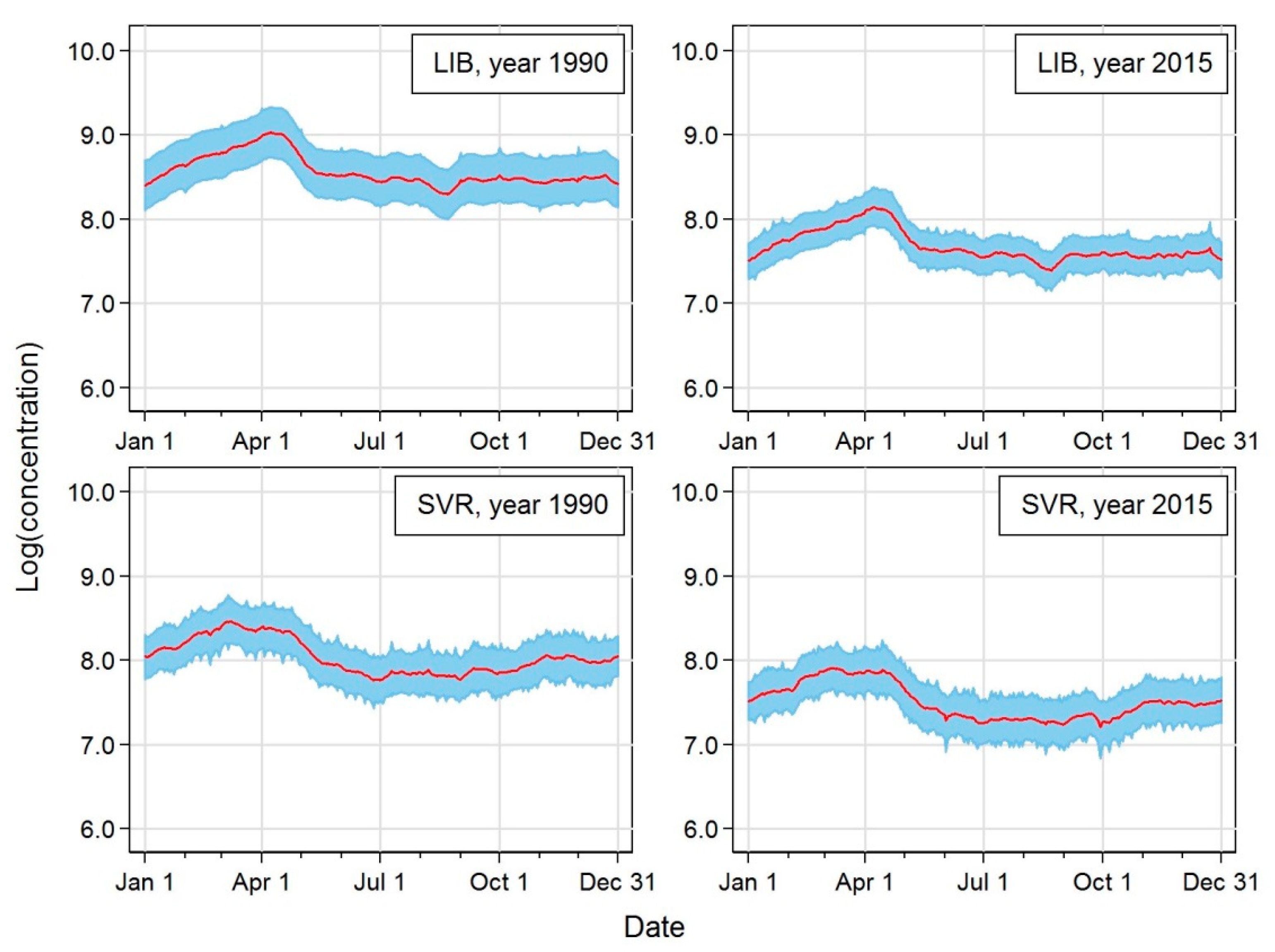
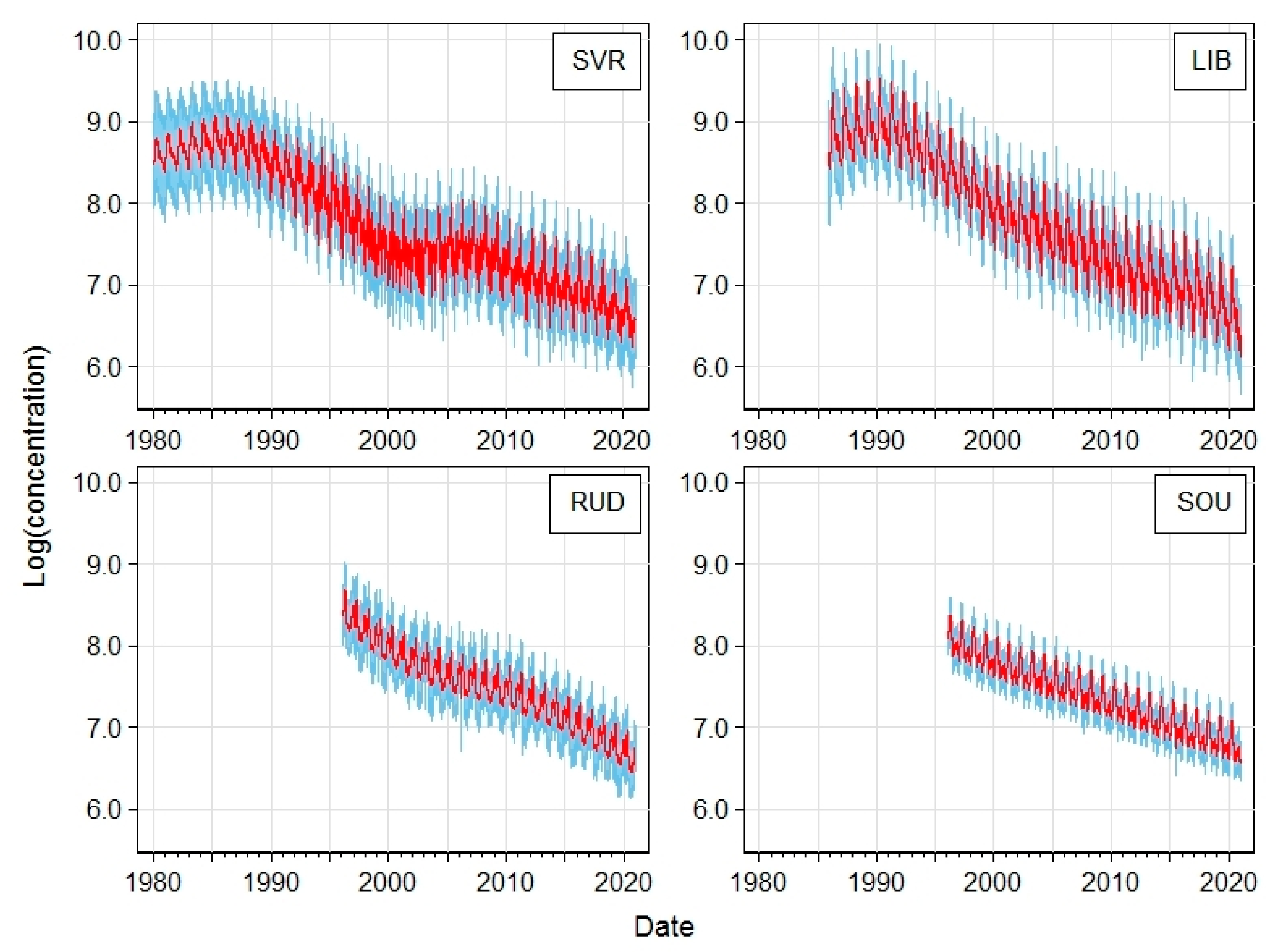
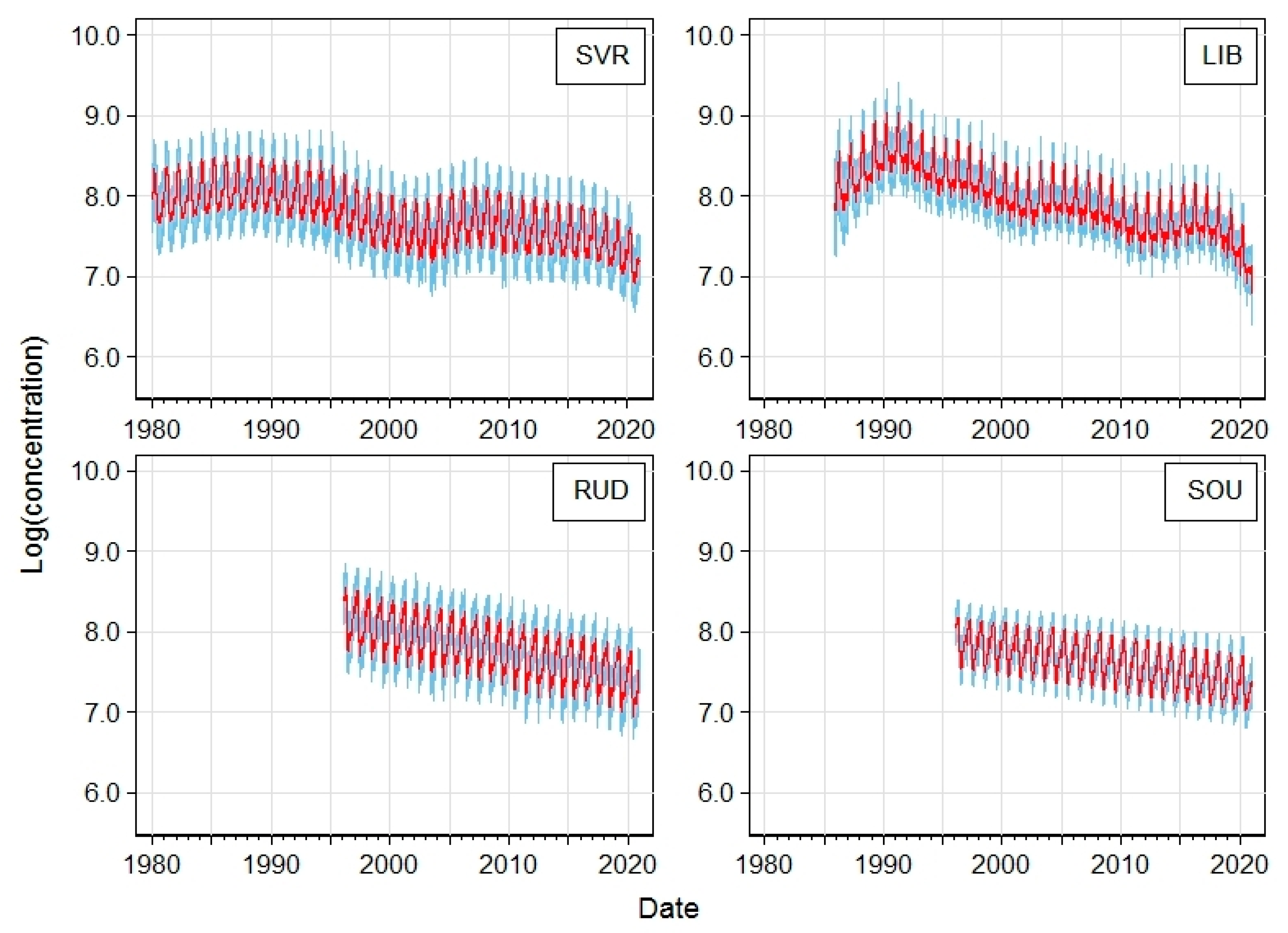
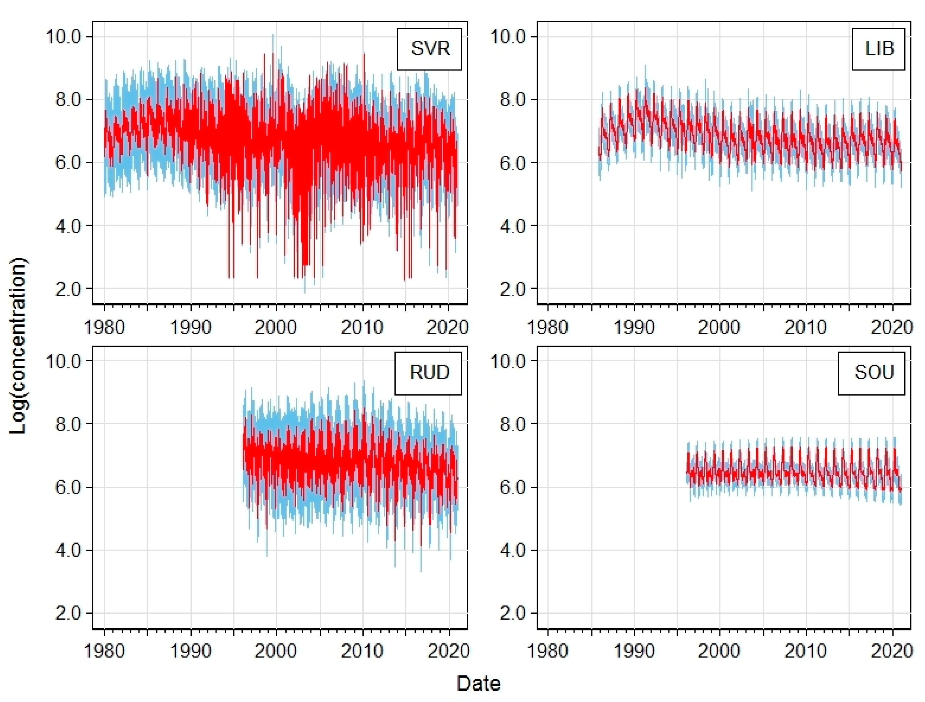
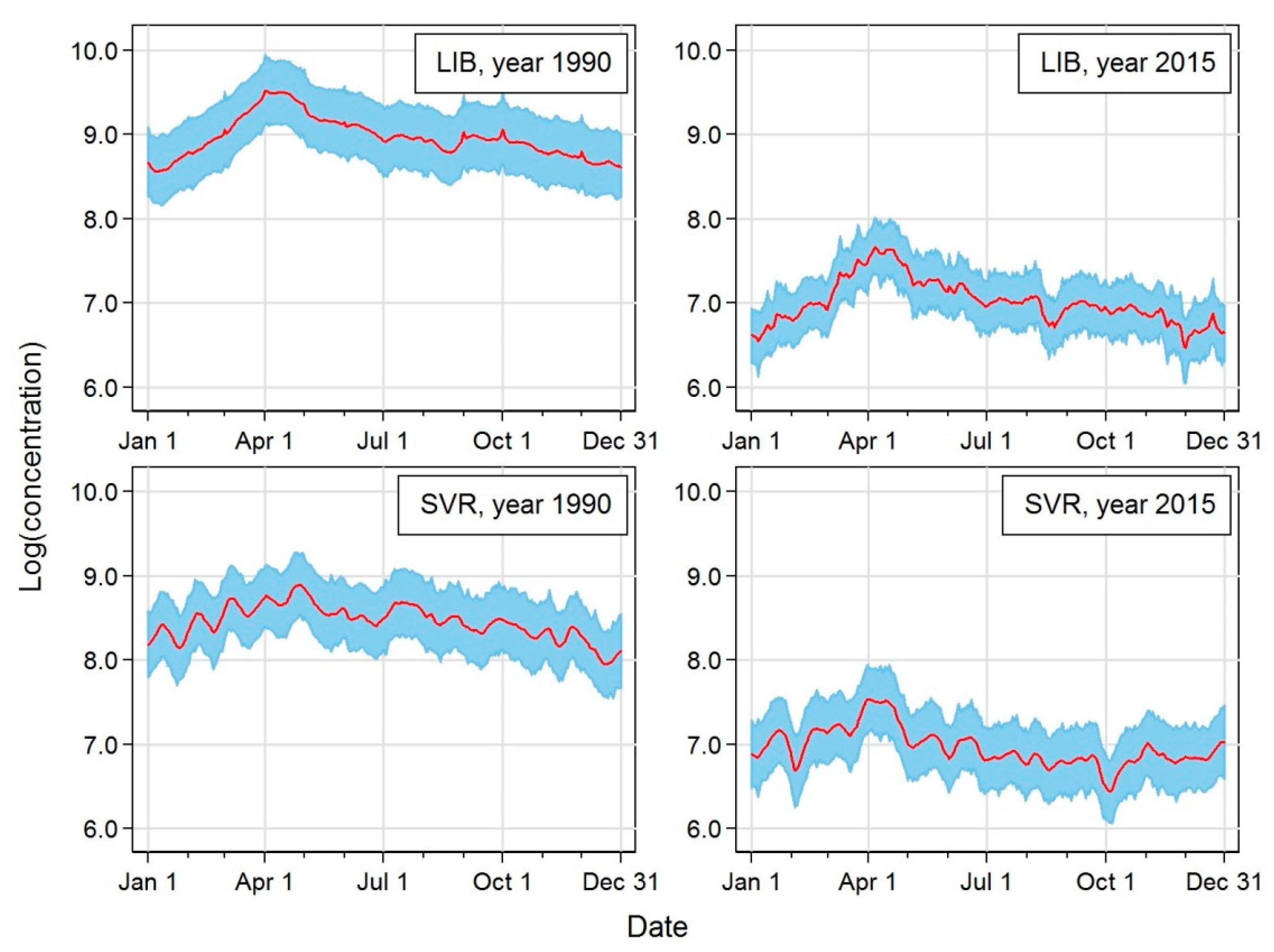
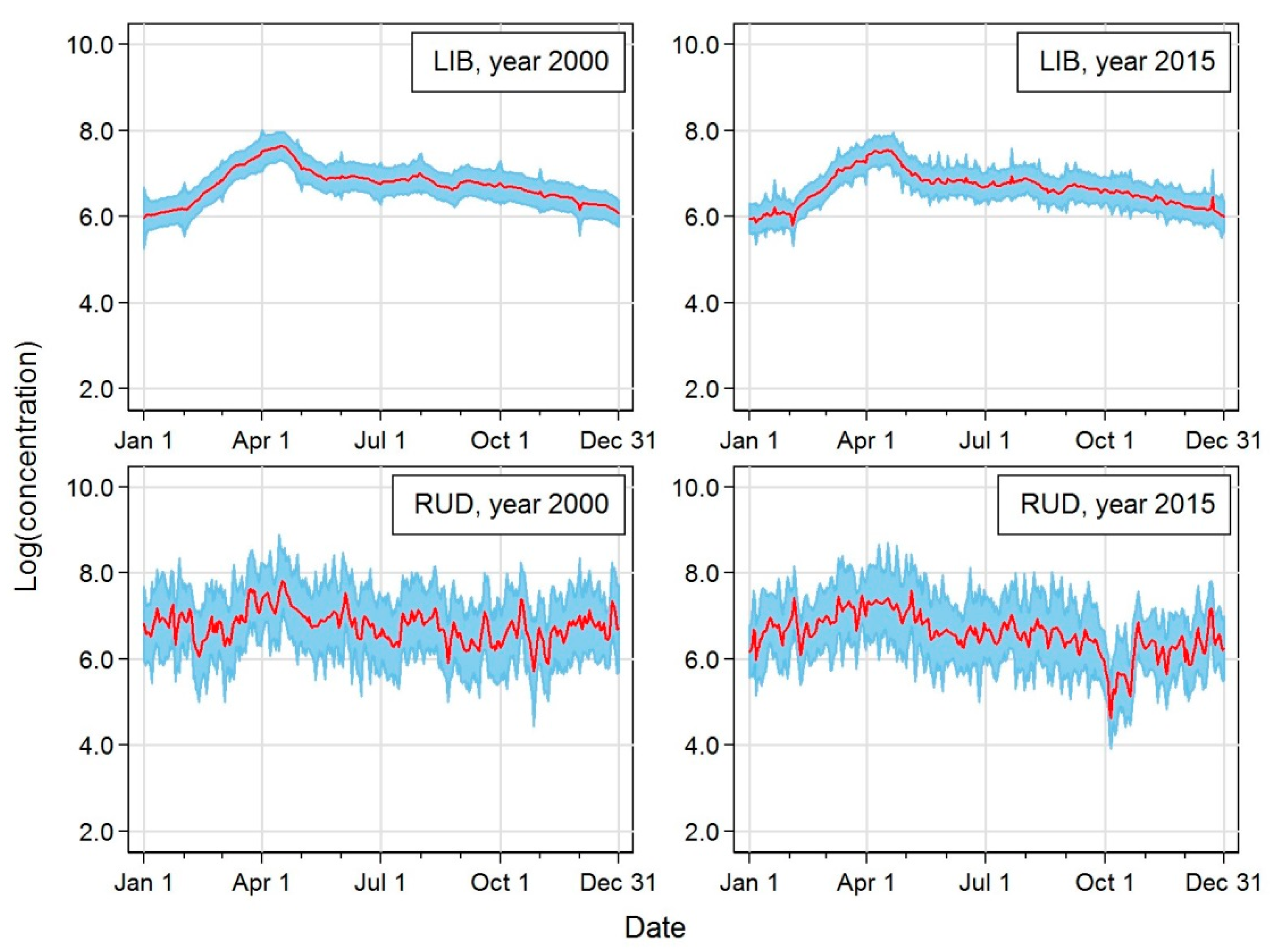
To regularise, the model is formulated in the Bayesian way, with complexity priors on structural parameters [48]. It is then identified or fitted (i.e., posterior distribution is obtained) using the numerically highly effective Integrated Nested Laplace Approximation (INLA) [39]. The use of INLA avoids the need for computationally costly Markov chain Monte Carlo sampling. The computational efficiency and flexibility of the INLA lead to its quickly increasing popularity [49]. For the computations, we use R [50] and the INLA library [39], utilising the elegant connection between the Matérn Gaussian random field and appropriate stochastic partial differential equation (SPDE) [51] to acquire computationally effective approximation for the interaction term. One substantial advantage of using INLA SW in this context is that the implicit aggregation from which data arise can be easily specified through a user-specified predictor matrix (available as one of many INLA flexible features). Apart from point estimates, we also assessed the uncertainty using 95% credible intervals. The model was fitted for each station separately, i.e., with stratification on station.

3. Results

Simple descriptive statistics characterising the measured values used as input data for modelling analysis are presented in Supplementary Table S1. The data are shown as annual sampling period-length-weighted geometric means. The principal results for SO₄²⁻, NO₃⁻ and NH₄⁺ concentrations in precipitation obtained from model (1) are shown in Figure 1, Figure 2 and Figure 3. In order to enable an easy visual comparison, we tried to adhere to the same scales for both axes for all ions as much as possible, except for the range for NH₄⁺, where we used a different minimum concentration (2 µg·m⁻³) than for two other ions (6 µg·m⁻³). A comparison of the general trends indicated that there are substantial differences between the three ions studied. Whereas the SO₄²⁻ and NO₃⁻ data series show a clear decline over time, though being more pronounced for SO₄²⁻ than NO₃⁻, the NH₄⁺ course is rather steady on larger time scales, evincing neither a decrease nor an increase over time.

The courses of SO₄²⁻ concentrations in precipitation (Figure 1) indicated the maxima reached at the turn of the 1990s at both the SVR and LIB sites, with a consequent steady decrease at LIB, showing interestingly amplifying ranges of concentrations towards recent years. At the SVR site, the decrease in SO₄²⁻ concentrations was interrupted at the beginning of the 2000s for a short period of some five years, showing a steady state with subsequent further decrease until now. The SO₄²⁻ courses at the RUD and SOU sites are shorter, nevertheless indicating similar decreases over the entire measurement period, though within much narrower ranges than the two previous sites, retaining a similar concentration spread for the entire period.

The courses of NO₃⁻ concentrations (Figure 2) indicated a decrease over time as well, though much milder than in the case of SO₄²⁻. The ranges of daily concentrations are similar for all four sites, unlike for SO₄²⁻. The SVR site showed a certain interruption in decrease in 2005–2008, similarly as for SO₄²⁻. The LIB site shows a kind of undulated decreasing trend of NO₃⁻³, with an abrupt drop in the last two years. The RUD and SOU NO₃⁻ concentration patterns evince similar decreases.

In contrast to the above ions, NH₄⁺ concentrations in precipitation (Figure 3) have more or less steady courses over time, with unprecedented broad ranges at the SVR site, the daily concentrations showing a very irregular pattern. Broad ranges—however, not as broad as for the SVR site—are found also for the RUD site, whereas the NH₄⁺ concentration pattern is much tighter for the LIB, and for the SOU site in particular.

Detailed views at individual ion courses over individual selected years, reflecting the air pollution levels in the past and present, are presented in Figure 4, Figure 5 and Figure 6. The overall one-year courses for SO₄²⁻ for LIB show very similar patterns with clear spring maxima in April both in 1990 and 2015, with the 2015 curve clearly situated much lower than the 1990 curve. SO₄²⁻ concentrations in SVR showed different patterns in 1990 and 2015, but dissimilar from the LIB site. The SO₄²⁻ concentrations in 2015 are much lower than those in 1990 (Figure 4).

In contrast, the NO₃⁻ concentration courses were very similar both at LIB and SVR and for both selected years of 1990 and 2015, with clear spring maxima in both selected years. The NO₃⁻ patterns were shifted lower for 2015 as compared to 1990 for both LIB and SVR. The credible intervals were narrower for NO₃⁻ than for SO₄²⁻ concentrations (Figure 5). For NH₄⁺ ions in LIB, the curves for both 2000 and 2015 were nearly identical with respect to both concentration values and shape with spring maxima in April, but very dissimilar in RUD, exhibiting oscillations over both years, with much wider credible intervals than LIB (Figure 6).

The 95% credible intervals are not overlapping for the SO₄²⁻ and NO₃⁻ concentrations for time patterns in 1990 and 2015 for the LIB and SVR sites (Figure 4 and Figure 5), indicating statistically significant decreases over time in these ion concentrations in precipitation. This is not the case for NH₄⁺, however, for the concentrations of which the 95% credible intervals for LIB and RUD sites in 2000 and 2015 do overlap, suggesting non-significant changes over time (Figure 6). Hence, within one measuring station, within the same ion, there is obviously a statistically significant decreasing trend for the SO₄²⁻ and NO₃⁻ concentrations, whereas it is not true for the NH₄⁺ concentrations in precipitation. Furthermore, the overlapping 95% credible intervals for individual examined ions suggest that concentration levels and time courses do not differ significantly between the measuring sites. However, we can still notice some differences, albeit statistically insignificant. For example, NO₃⁻ concentrations show higher values at the LIB site and partly also at the RUD site than at other sites (Figure 2), and SO₄²⁻ concentrations show a faster decrease in time at the LIB and RUD sites compared to SOU (Figure 1).

4. Discussion

4.1. Specific Comments on the Observed Patterns

Decreasing trends in SO₄²⁻ and somewhat lower decreases in NO₃⁻ concentrations in precipitation are in line with observations elsewhere and reflect the decrease in SO₂ and NO_x emissions due to stringent and effective countermeasures taken in Europe [21] and North America [16]. In contrast, NH₄⁺ concentrations in precipitation exhibit a more or less steady state at the examined stations, which reflects the fact that unlike SO₂ and NO_x, NH₃ is not a criteria pollutant required by the EU legislation in force [52], and so the emission reductions of NH₃ appear problematic in reality [53]. This is also reflected in the increasing relative contribution of NH₄⁺ as compared to NO₃⁻ to atmospheric deposition of reactive nitrogen reported both from Europe [8,54], including the Czech Republic [38] and other countries worldwide [55,56]. It is necessary to remark, however, that this is not the case everywhere, and that in particular, European countries loaded with high NH₃ emissions in the past, such as Belgium/Flanders, The Netherlands and France, reported the opposite trend [57,58,59].

Temporal variations in major ion concentrations with spring maxima for Europe were noted and reported earlier, with an unclear explanation [60]. Interestingly, major ions in precipitation frequently show similar seasonal variations though they originate from different sources [61]. We saw spring maxima for all three ions examined at the LIB site for both past and current measurements, though the occurrence of the spring maximum was not the case for all stations.

The visible drop in NO₃⁻ concentrations observed at the LIB site in the past two years is likely to be due to the COVID-19 pandemic and related lockdowns with subsequent decreases in NO_x in ambient air (precursors of NO₃⁻ in precipitation), which was reported from many urban regions in Europe [62,63,64], including the Czech Republic [65]. A decrease in the number of cars operated in urban areas due to people being in home offices actually resulted in substantial NO_x emission decreases in many cities, including Prague [66].

4.2. Problems in Long-Term Assessment Arising from Changes in Monitoring with Respect to Sampling Period Length

In the evaluation of long-term ambient air pollution trends, a general problem remains to be solved. This problem relates to changing sampling periods over time [67]. This is of general interest since precipitation samples for ion analysis are generally collected with different sampling interval lengths, typically days, weeks or months, but other lengths might arise for logistic and other practical reasons [68]. The collection length can be different not only among different sampling sites (stations), it can also change during the course of time even for the same station (e.g., in relationship with the development and expansion of the nation-wide ambient air quality monitoring network, changes related to monitoring budget fluctuations, etc). Temporal changes are obviously slow and hence they might be perceived as not very important for studies conducted at shorter time intervals (specifically, over months to a few years). They are of substantial importance, however, when one wants to retrieve information on long-term trends—monitoring network maturation (in the form of a gradual tendency toward shorter sample collection periods) definitely comes into play as a nuisance factor.

An additional problem comes with occasional missing values interspersed among valid observations [69,70]. Indeed, looking at raw data amounts directly to looking through a distorting filter whose properties change over time. Furthermore, even for short-term studies, it is not unusual to have incompatibilities in the sampling period among the stations spatially at the same time. It seems that many practical assessments lack appreciation of the extent of the problem the sampling interval inhomogeneities bring into data analysis and interpretation. It is a nuisance (purely artificial) factor that is not connected with the studied process of ion concentration. Surely enough, it is of no interest. Nevertheless, it modulates the output data in a complex way that might prevent direct compatibility of measurements in both time and space.

Direct comparison of different collection lengths (e.g., daily and monthly data) is, of course, impossible [71]. A simple reaction might be to reduce the resolution to the length of the coarsest collection interval (e.g., month, if monthly and weekly data are compared). This is not only deficient (it leads to an information loss), it might not be a feasible approach (if there is a phase shift between the two periods). Alternatively, many published analyses resigned to the original data resolution and compare only highly aggregated data (e.g., annual averages) for which the effect of sampling interval incompatibilities is small or negligible [72,73].

Such an approach, however, inevitably results in a substantial waste of information. This crude treatment prevents the detailed inspection inside intra-annual (seasonal) patterns and their changes over the years of monitoring. It is more appropriate to remove observational process complexities and irregularities by estimating concentration time series in a unified finer-than-year resolution in an objective way and then compare their properties across time and space. This amounts to the reconstruction of the concentration at a finer time resolution for all stations of interest in a unified and principled manner. The approach based on the statistical removal of the distorting filter is indeed possible and relatively straightforward, as its properties (based on sampling collection length) are known precisely.

The sub-year scale of ion precipitation concentration changes is exactly what we aim at in this work. For this, we have to adjust first for the sampling interval inhomogeneities both across and within stations. We achieve this adjustment by a formalised statistical modelling that allows us to reconstruct estimated time series of ion concentration in a unified time resolution (i.e., the same time-step for all estimates both within and across stations). We choose the daily resolution for the estimates. Beyond presenting and interpreting the concrete concentration series reconstructions, we describe a powerful but relatively simple framework for the formalised Bayesian statistical modelling that allows reconstruction. Seen from a broader viewpoint, the reconstruction amounts to the disaggregation of originally irregularly aggregated time series via a fully specified Bayesian model (with complexity penalised priors analogous to the roughness penalties customarily used in the traditional smoothing).

4.3. Overall Evaluation

In our study, we provide insight into the daily behaviour of major inorganic ions in precipitation samples collected on a monthly or weekly basis. This detailed insight was achieved by decomposing the data series gained in longer-term exposures (employed as a standard in most measuring networks) into detailed daily concentration patterns using a relevant statistical approach to reveal the information embedded in monthly or weekly cumulative values, hidden so far in these “averaged” data. This type of analysis is useful for multiple purposes indicated briefly below.

First, we are able to obtain information on daily precipitation concentrations from samples collected via longer than a day exposure—in our case, via cumulative sampling over a month or a week. At the same time, it is important to realise the obvious fact that what we attain is an estimate of the daily concentration trajectory. Nevertheless, it is an optimal estimate, justified by the fact that it arises from formally derived posterior distribution [74] formulated in an objective way that removes artefacts and inhomogeneities of the complex sampling procedure. This appears very useful as we can gain information in a more detailed time resolution, saving money and efforts on daily sampling, which is usually impractical and not achievable, specifically in rural areas, where precipitation chemistry sampling is frequently operated. These sites are mostly not easily accessible locations in mountain areas, usually in complex forested terrain, sometimes in remote regions. For practical purposes, it will be important to consider possible savings together with increased imprecision of the estimates arising from longer sampling times when creating a measurement network. The principles of statistical theory of experimental design apply directly here [75].

Second, we can explore the daily behaviour of various aspects of precipitation chemistry. For instance, using the daily concentration estimates, we can appreciate both the magnitude and shape of ion concentration trajectories. Furthermore, from this type of analysis, we gain comparable shapes and magnitudes of the concentrations, the magnitudes being the natural logarithms of estimated daily concentrations. Third, we can consider re-aggregation of these earlier disintegrated daily concentrations into a time series of some lower but constant resolution of interest. Furthermore, we can easily estimate concentration averages for various practically relevant time periods, such as vegetation seasons or phenological phases, etc., meaningful with respect to the impact of the studied substances (in our case, sulphur and nitrogen) on vegetation and ecosystems, either via deposition or uptake pathways.

Last but not least, this kind of analysis might serve as a valuable tool for a kind of logical verification of measured data, as these can be assumed to follow a distinguished pattern. In this point, we can refer to Figure 3, showing an extremely strange and messy pattern of NH₄⁺ concentrations at the SVR site, quite different from NH₄⁺ behaviour pattern at other sites, which might indicate some problems in measurements and provoke a check of sampling and measuring operating procedures. In any case, such a highly disputable precipitation chemistry pattern requires further attention and scrutinising of possible causes, which might reveal either a systematic error in sampling or indicate a sort of interesting feature deserving further exploration.

In particular, such an analysis is important amid an ongoing global environmental change bringing substantial alterations in precipitation patterns [76,77,78], and with respect to carrying out broader syntheses exploring possible ambient air quality impacts on the environment and ecosystems, where the obtained results may serve as valuable inputs describing atmospheric deposition as an important driver of air pollution.

5. Conclusions and Outlook

We explored the long-term dynamics of sulphates (SO₄²⁻), nitrates (NO₃⁻) and ammonia (NH₄⁺) ions measured in precipitation within a nation-wide precipitation chemistry monitoring network in the Czech Republic. The raw data span dozens of years and reflect the evolution of the measurement network; the collection periods are changing throughout time (the collection intervals tend to shorten, overall) and are generally different for different stations. Therefore, we formulated a Bayesian statistical model that allows for the estimation of concentration in daily resolution. The model was fitted using the INLA approach for each station of interest separately (formally, we are stratifying on station) and the course of the dynamics was reconstructed as a time series with an equidistant daily step. Using the INLA approach enabled us to reconstruct the daily courses of major ion concentrations in precipitation sampled over different exposure time periods (weekly, monthly). These reconstructed daily patterns are useful for numerous reasons and offer a wide range of possibilities for further exploration, such as (1) gaining more detailed patterns from longer exposure sampling periods relevant predominantly for rural and remote regions, (2) exploration of the daily behaviour of precipitation chemistry at different sites benefitting from the fact that both shapes and magnitudes are comparable, (3) aggregation of the earlier disintegrated daily concentrations into selected time periods relevant with respect to phenology or ecology and (4) logical verification of measured data.

Our detailed analysis revealed sharp decreases in SO₄²⁻, milder decreases in NO₃⁻ and steady states in NH₄⁺ concentrations in precipitation. With respect to within-year courses, spring maxima in April were found for all major ions at the LIB site and for NO₃⁻ at the SVR site, for both past and current samples. In contrast, no distinct seasonal behaviour was recorded for NH₄⁺ at the RUD site and SO₄²⁻ at the SVR site. It will be interesting to use in the future an approach similar to the (expanded version of the) reconstruction presented in this paper for estimating the relationship between the concentrations of gaseous and water concentrations of naturally related compounds (such as SO₂ and NO_x on one side, and sulphates and nitrates on the other).

References

1. Seinfeld, J.H.; Pandis, S.N. Atmospheric Chemistry and Physics; John Wiley: New York, NY, USA, 1998; p. 1326. [Google Scholar]
2. Pacyna, J.M. Atmospheric Deposition. In Encyclopedia of Ecology; Academic Press: Cambridge, MA, USA, 2008; pp. 275–285. Available online: https://www.sciencedirect.com/science/article/pii/B9780080454054002585 (accessed on 10 April 2022).
3. Galloway, J.N.; Cowling, E.B. The Effects of Precipitation on Aquatic and Terrestrial Ecosystems: A Proposed Precipitation Chemistry Network. J. Air Pollut. Control Assoc. 1978, 28, 229–235. [Google Scholar] [CrossRef] [Green Version]
4. Sirois, A.; Vet, R.; Lamb, D.A. Comparison of the Precipitation Chemistry Measurements Obtained by the CAPMoN and NADP/NTN Networks. Environ. Monit. Assess. 2000, 62, 273–303. [Google Scholar] [CrossRef]
5. Wetherbee, G.A.; Shaw, M.J.; Latysh, N.E.; Lehmann, C.M.B.; Rothert, J.E. Comparison of precipitation chemistry measurements obtained by the Canadian Air and Precipitation Monitoring Network and National Atmospheric Deposition Program for the period 1995–2004. Environ. Monit. Assess. 2010, 164, 111–132. [Google Scholar] [CrossRef] [PubMed]
6. Tørseth, K.; Aas, W.; Breivik, K.; Fjæraa, A.M.; Fiebig, M.; Hjellbrekke, A.G.; Lund, M.C.; Solberg, S.; Yttri, K.E. Introduction to the European Monitoring and Evaluation Programme (EMEP) and observed atmospheric composition change during 1972–2009. Atmos. Chem. Phys. 2012, 12, 5447–5481. [Google Scholar] [CrossRef] [Green Version]
7. Amodio, M.; Catino, S.; Dambruoso, P.R.; de Gennaro, G.; di Gilio, A.; Giungato, P.; Laiola, E.; Marzocca, A.; Mazzone, A.; Sardaro, A.; et al. Atmospheric Deposition: Sampling Procedures, Analytical Methods, and Main Recent Findings from the Scientific Literature. Adv. Meteorol. 2014, 2014, 161730. [Google Scholar] [CrossRef]
8. Vet, R.; Artz, R.S.; Carou, S.; Shaw, M.; Ro, C.-U.; Aas, W.; Baker, A.; Bowersox, V.C.; Dentener, F.; Galy-Lacaux, C.; et al. A global assessment of precipitation chemistry and deposition of sulphur, nitrogen, sea salt, base cations, organic acids, acidity and pH, and phosphorus. Atmos. Environ. 2014, 93, 3–10. [Google Scholar] [CrossRef]
9. Seinfeld, J.H. Air Pollution: A Half Century of Progress. AIChE J. 2004, 50, 1096–1108. [Google Scholar] [CrossRef]
10. Erisman, J.W.; Draaijers, G.P.J. Atmospheric Deposition: In Relation to Acidification and Eutrophication; Studies in Environmental Science 63; Elsevier: Amsterdam, The Netherlands, 1995. [Google Scholar]
11. Forsius, M.; Posch, M.; Holmberg, M.; Vuorenmaa, J.; Kleemola, S.; Augustaitis, A.; Beudert, B.; Bochenek, W.; Clarke, N.; de Wit, H.A.; et al. Assessing critical load exceedances and ecosystem impacts of anthropogenic nitrogen and sulphur deposition at unmanaged forested catchments in Europe. Sci. Total Environ. 2021, 753, 141791. [Google Scholar] [CrossRef]
12. Lovett, G.M.; Burns, D.A.; Driscoll, C.T.; Jenkins, J.C.; Mitchell, M.J.; Rustad, L.; Shanley, J.B.; Likens, G.E.; Haeuber, R. Who needs environmental monitoring? Front. Ecol. Environ. 2007, 5, 253–260. [Google Scholar] [CrossRef]
13. Likens, G.E.; Butler, T.J.; Claybrooke, R.; Vermeylen, F.; Larson, R. Long-term monitoring of precipitation chemistry in the U.S.: Insights into changes and condition. Atmos. Environ. 2021, 245, 118031. [Google Scholar] [CrossRef]
14. Weatherhead, E.C.; Reinsel, G.C.; Tiao, G.C.; Meng, X.-L.; Choi, D.; Cheang, W.-K.; Keller, T.; DeLuisi, J.; Wuebbles, D.J.; Kerr, J.B.; et al. Factors affecting the detection of trends: Statistical considerations and applications to environmental data. J. Geophys. Res. 1998, 103, 17149–17161. [Google Scholar] [CrossRef]
15. Farmer, G.; Barthelmie, R.; Davies, T.; Brimblecombe, P.; Kelly, P.M. Relationships between concentration and deposition of nitrate and sulphate in precipitation. Nature 1987, 328, 787–789. [Google Scholar] [CrossRef]
16. Lehmann, C.M.B.; Bowersox, V.C.; Larson, S.M. Spatial and temporal trends of precipitation chemistry in the United States, 1985–2002. Environ. Pollut. 2005, 135, 347–361. [Google Scholar] [CrossRef]
17. Staelens, J.; Wuyts, K.; Adriaenssens, S.; Van Avermaet, P.; Buysse, H.; Van den Bril, B.; Roekens, E.; Ottoy, J.-P.; Verheyen, K.; Thas, O.; et al. Trends in atmospheric nitrogen and sulphur deposition in northern Belgium. Atmos. Environ. 2012, 49, 186–196. [Google Scholar] [CrossRef]
18. Waldner, P.; Marchetto, A.; Thimonier, A.; Schmitt, M.; Rogora, M.; Granke, O.; Mues, V.; Hansen, K.; Karlsson, G.P.; Žlindra, D.; et al. Detection of temporal trends in atmospheric deposition of inorganic nitrate and sulphate to forests in Europe. Atmos. Environ. 2014, 95, 363–374. [Google Scholar] [CrossRef] [Green Version]
19. Fanta, J. Rehabilitating degraded forests in Central Europe into self-sustaining forest ecosystems. Ecol. Eng. 1997, 8, 289–297. [Google Scholar] [CrossRef]
20. Moldan, B.; Hak, T. Environment in the Czech Republic: A Positive and Rapid Change. Environ. Sci. Technol. 2007, 41, 358–362. [Google Scholar] [CrossRef] [Green Version]
21. EEA. Air Quality in Europe—2020 Report; European Environmental Agency, No 09/2020; EEA: Copenhagen, Denmark, 2020. [Google Scholar]
22. Keresztesi, A.; Birsan, M.-V.; Nita, I.-A.; Bodor, Z.; Szep, R. Assessing the neutralisation, wet deposition and source contributions of the precipitation chemistry over Europe during 2000–2017. Environ. Sci. Eur. 2019, 31, 50. [Google Scholar] [CrossRef] [Green Version]
23. Bruce, A.; Bray, D.; Hopkin, K.; Johnson, A.; Lewis, J.; Raff, M.; Roberts, K.; Walter, P. Essential Cell Biology, 4th ed.; Garland Science, Taylor & Francis Group, LLC: New York, NY, USA, 2014. [Google Scholar]
24. Likens, G.E.; Bormann, F.H.; Johnson, N.M. Interactions between major biogeochemical cycles in terrestrial ecosystems. In Some Perspectives of the Major Biogeochemical Cycles; Likens, G.E., Ed.; SCOPE: Chichester, UK, 1981; pp. 93–112. [Google Scholar]
25. Galloway, J.N.; Dentener, F.J.; Capone, D.G.; Boyer, E.W.; Howarth, R.W.; Seitzinger, S.P.; Asner, G.P.; Cleveland, C.C.; Green, P.A.; Holland, E.A.; et al. Nitrogen cycles: Past, present, and future. Biogeochemistry 2004, 70, 153–226. [Google Scholar] [CrossRef]
26. Galloway, J.N.; Townsend, A.R.; Erisman, J.W.; Bekunda, M.; Cai, Z.; Freney, J.R.; Martinelli, L.A.; Seitzinger, S.P.; Sutton, M.A. Transformation of the nitrogen cycle: Recent trends, questions and potential solutions. Science 2008, 320, 889–892. [Google Scholar] [CrossRef] [Green Version]
27. Fowler, D.; Pyle, J.A.; Raven, J.A.; Sutton, M.A. The global nitrogen cycle in the twenty-first century: Introduction. Philos. Trans. R. Soc. B Biol. Sci. 2013, 368, 20130165. [Google Scholar] [CrossRef] [PubMed]
28. Bridges, K.S.; Jickells, T.D.; Davies, T.D.; Zeman, Z.; Hůnová, I. Aerosol, precipitation and cloud water observations on the Czech Krusne Hory plateau adjacent to a heavily industrialised valley. Atmos. Environ. 2002, 36, 353–360. [Google Scholar] [CrossRef]
29. Bridgman, H.A.; Davies, T.D.; Jickells, T.; Hůnová, I.; Tovey, K.; Bridges, K.; Surapipith, V. Air pollution in the Krusne hory region, Czech Republic during the 1990s. Atmos. Environ. 2002, 36, 3375–3389. [Google Scholar] [CrossRef]
30. Hůnová, I. Ambient Air Quality in the Czech Republic: Past and Present. Atmosphere 2020, 11, 214. [Google Scholar] [CrossRef] [Green Version]
31. Hůnová, I. Ambient air quality for the territory of the Czech Republic in 1996–1999 expressed by three essential factors. Sci. Total Environ. 2003, 303, 245–251. [Google Scholar] [CrossRef]
32. Hůnová, I.; Kurfürst, P.; Maznová, J.; Coňková, M. The contribution of occult precipitation to sulphur deposition in the Czech Republic. Erdkunde 2011, 65, 247–259. [Google Scholar] [CrossRef]
33. Hůnová, I.; Kurfürst, P.; Baláková, L. Areas under high ozone and nitrogen loads are spatially disjunct in Czech forests. Sci. Total Environ. 2019, 656, 567–575. [Google Scholar] [CrossRef]
34. Hůnová, I.; Brabec, M.; Malý, M.; Valeriánová, A. Long-term trends in fog occurrence in the modern-day Czech Republic, Central Europe. Sci. Total Environ. 2020, 711, 135018. [Google Scholar] [CrossRef]
35. CHMI. Air pollution in the Czech Republic in 2019; Czech Hydrometeorological Institute: Prague, Czech Republic, 2020. [Google Scholar]
36. Hůnová, I.; Šantroch, J.; Ostatnická, J. Ambient air quality and deposition trends at rural stations in the Czech Republic during 1993–2001. Atmos. Environ. 2004, 38, 887–898. [Google Scholar] [CrossRef]
37. Hůnová, I.; Maznová, J.; Kurfürst, P. Trends in atmospheric deposition fluxes of sulphur and nitrogen in Czech forests. Environ. Pollut. 2014, 184, 668–675. [Google Scholar] [CrossRef]
38. Hůnová, I.; Kurfürst, P.; Stráník, V.; Modlík, M. Nitrogen deposition to forest ecosystems with focus on its different forms. Sci. Total Environ. 2017, 575, 791–798. [Google Scholar] [CrossRef] [PubMed]
39. Rue, H.; Martino, S.; Chopin, N. Approximate Bayesian Inference for Latent Gaussian Models Using Integrated Nested Laplace Approximations (with discussion). J. R. Stat. Soc. Series B 2009, 71, 319–392. [Google Scholar] [CrossRef]
40. Sanyal, S.; Rochereau, T.; Maesano, C.N.; Com-Ruelle, L.; Annesi-Maesano, I. Long-Term Effect of Outdoor Air Pollution on Mortality and Morbidity: A 12-Year Follow-Up Study for Metropolitan France. Int. J. Environ. Res. Public Health 2018, 15, 2487. [Google Scholar] [CrossRef] [PubMed] [Green Version]
41. Shaddick, G.; Thomas, M.L.; Amini, H.; Broday, D.; Cohen, A.; Frostad, J.; Green, A.; Gumy, S.; Liu, Y.; Martin, R.V.; et al. Data Integration for the Assessment of Population Exposure to Ambient Air Pollution for Global Burden of Disease Assessment. Environ. Sci. Technol. 2018, 52, 9069–9078. [Google Scholar] [CrossRef]
42. Limpert, E.; Stahel, W.; Abbt, M. Lognormal distributions across the sciences: Keys and clues. BioScience 2001, 51, 341–352. [Google Scholar] [CrossRef]
43. Shumway, R.H.; Stoffer, D.S. Time Series Analysis and Its Applications: With R Examples, 4th ed.; Springer: Cham, Switzerland, 2017. [Google Scholar]
44. Hastie, T.; Tibshirani, R. Generalized Additive Models; Chapman & Hall/CRC: Boca Raton, FL, USA, 1990. [Google Scholar]
45. Wood, S.N. Generalized Additive Models: An Introduction with R, 2nd ed.; Chapman & Hall/CRC: New York, NY, USA, 2017. [Google Scholar]
46. Rawlings, J.O.; Pantula, S.G.; Dickey, D.A. Applied Regression Analysis; Springer: New York, NY, USA, 1998. [Google Scholar]
47. Rue, H.; Held, L. Gaussian Markov Random Fields: Theory and Applications; Monographs on Statistics and Applied Probability; Chapman & Hall: London, UK, 2005; Volume 104. [Google Scholar]
48. Simpson, D.P.; Rue, H.; Riebler, A.; Martins, T.G.; Sørbye, S.H. Penalising model component complexity: A principled, practical approach to constructing priors (with discussion). Stat. Sci. 2017, 32, 1–28. [Google Scholar] [CrossRef]
49. Bakka, H.; Rue, H.; Fuglstad, G.; Riebler, A.; Bolin, D.; Illian, J.; Krainski, E.; Simpson, D.; Lindgren, F. Spatial modelling with R-INLA: A review. WIRE Comput. Stat. 2018, 10, e1443. [Google Scholar]
50. R Core Team. R: A Language and Environment for Statistical Computing; R Foundation for Statistical Computing: Vienna, Austria, 2022; Available online: www.R-project.org (accessed on 14 May 2022).
51. Lindgren, F.; Rue, H.; Lindström, J. An explicit link between Gaussian fields and Gaussian Markov random fields: The SPDE approach (with discussion). J. R. Stat. Soc. Series B 2011, 73, 423–498. [Google Scholar] [CrossRef] [Green Version]
52. EC. Directive 2008/50/EC of the European Parliament and of the Council of 21 May 2008 on Ambient Air Quality and Cleaner Air for Europe; EC: New York, NY, USA, 2008. [Google Scholar]
53. Sutton, M.A.; Reis, S.; Baker, S.M. (Eds.) Atmospheric Ammonia; Springer: Dordrecht, The Netherlands, 2009. [Google Scholar]
54. Fagerli, H.; Aas, W. Trends in nitrogen in air and precipitation: Model results and observations at EMEP sites in Europe, 1980–2003. Environ. Pollut. 2008, 154, 448–461. [Google Scholar]
55. Du, E.; de Vries, W.; Galloway, J.N.; Hu, X.; Fang, J. Changes in wet nitrogen deposition in the United States between 1985 and 2012. Environ. Res. Lett. 2014, 9, 095004. [Google Scholar] [CrossRef]
56. Li, X.; Shi, H.; Xu, W.; Liu, W.; Wang, X.; Hou, L.; Feng, F.; Yuan, W.; Li, L.; Xu, H. Seasonal and spatial variations of bulk nitrogen deposition and the impacts on the carbon cycle in the arid/semiarid grassland of Inner Mongolia, China. PLoS ONE 2015, 10, e0144689. [Google Scholar] [CrossRef] [PubMed]
57. Boxman, A.W.; Peters, R.C.J.H.; Roelofs, J.G.M. Long-term changes in atmospheric N and S throughfall deposition and effects on soil solution chemistry in a Scots pine forest in the Netherlands. Atmos. Environ. 2008, 156, 1252–1259. [Google Scholar] [CrossRef] [PubMed]
58. Verstraeten, A.; Neirynck, J.; Genouw, G.; Cools, N.; Roskams, P.; Hens, M. Impact of declining atmospheric deposition on forest soil solution chemistry in Flanders, Belgium. Atmos. Environ. 2012, 62, 50–63. [Google Scholar] [CrossRef]
59. Pascaud, A.; Sauvage, S.; Coddeville, P.; Nicolas, M.; Croisé, L.; Mezdour, A.; Probst, A. Contrasted spatial and long-term trends in precipitation chemistry and deposition fluxes at rural stations in France. Atmos. Environ. 2016, 146, 28–43. [Google Scholar] [CrossRef] [Green Version]
60. Fuhrer, J. Study of Acid Deposition in Switzerland: Temporal Variation in the Ionic Composition of Wet Precipitation at Rural Sites during 1983-1984. Environ. Pollut. 1986, 12, 111–129. [Google Scholar] [CrossRef]
61. Irwin, J.G.; Williams, M.L. Acid Rain: Chemistry and Transport. Environ. Pollut. 1988, 50, 29–59. [Google Scholar] [CrossRef]
62. Lovarelli, D.; Conti, C.; Finzi, A.; Bacenetti, J.; Guarino, M. Describing the trend of ammonia, particulate matter and nitrogen oxides: The role of livestock activities in northern Italy during COVID-19 quarantine. Environ. Res. 2020, 191, 110048. [Google Scholar] [CrossRef]
63. Menut, L.; Bessagnet, B.; Siour, G.; Mailler, S.; Pennel, R.; Cholakian, A. Impact of lockdown measures to combat COVID-19 on air quality over western Europe. Sci. Total Environ. 2020, 741, 140426. [Google Scholar] [CrossRef]
64. Naethe, P.; Delaney, M.; Julitta, T. Changes of NOx in urban air detected with monitoring VIS-NIR field spectrometer during the coronavirus pandemic: A case study in Germany. Sci. Total Environ. 2020, 748, 141286. [Google Scholar]
65. Vichova, K.; Veselik, P.; Heinzova, R.; Dvoracek, R. Road Transport and Its Impact on Air Pollution during the COVID-19 Pandemic. Sustainability 2021, 13, 11803. [Google Scholar] [CrossRef]
66. CHMI. Air Pollution in the Czech Republic in 2020; Czech Hydrometeorological Institute: Prague, Czech Republic, 2021. [Google Scholar]
67. Galloway, J.N.; Likens, G.E. The collection of precipitation for chemical analysis. Tellus 1978, 30, 71–82. [Google Scholar] [CrossRef] [Green Version]
68. Krupa, S. Sampling and physico-chemical analysis of precipitation: A review. Environ. Pollut. 2002, 120, 565–594. [Google Scholar] [CrossRef]
69. Little, R.J.A.; Rubin, D.B. Statistical Analysis with Missing Data; Wiley: New York, NY, USA, 1987. [Google Scholar]
70. Schafer, J.L. Analysis of Incomplete Multivariate Data; Monographs on Statistics and Applied Probability; Chapman & Hall: London, UK, 1997; Volume 72. [Google Scholar]
71. Sirois, A.; Vet, R. The Precision of Precipitation Chemistry Measurements in the Canadian Air and Precipitation Monitoring Network (CAPMoN). Environ. Monit. Assess. 1999, 57, 301–329. [Google Scholar] [CrossRef]
72. Schwab, J.J.; Casson, P.; Brandt, R.; Husain, L.; Dutkewicz, V.; Wolfe, D.; Demerjian, K.L.; Civerolo, K.L.; Rattigan, O.V.; Felton, H.D.; et al. Atmospheric Chemistry Measurements at Whiteface Mountain, NY: Cloud Water Chemistry, Precipitation Chemistry, and Particulate Matter. Aerosol Air Qual. Res. 2016, 16, 841–854. [Google Scholar] [CrossRef] [Green Version]
73. Itahashi, S.; Yumimoto, K.; Uno, I.; Hayami, H.; Fujita, S.-I.; Pan, Y.; Wang, Y. A 15-year record (2001–2015) of the ratio of nitrate to non-sea-salt sulfate in precipitation over East Asia. Atmos. Chem. Phys. 2018, 18, 2835–2852. [Google Scholar] [CrossRef] [Green Version]
74. Gelman, A.; Carlin, J.B.; Stern, H.S.; Rubin, D.B. Bayesian Data Analysis, 2nd ed.; Chapman & Hall/CRC: Boca Raton, FL, USA, 2003. [Google Scholar]
75. Montgomery, D.C. Design and Analysis of Experiments, 8th ed.; John Wiley & Sons, Inc.: Hoboken, NJ, USA, 2013. [Google Scholar]
76. Jacob, D.J.; Winner, D.A. Effect of climate change on air quality. Atmos. Environ. 2009, 43, 51–63. [Google Scholar] [CrossRef] [Green Version]
77. Jones, J.M.; Davies, T.D. The influence of climate on air and precipitation chemistry over Europe and downscaling applications to future acidic deposition. Clim. Res. 2000, 14, 7–24. [Google Scholar] [CrossRef] [Green Version]
78. von Schneidemesser, E.; Monks, P.S.; Allan, J.D.; Bruhwiler, L.; Forster, P. Chemistry and the Linkages between Air Quality and Climate Change. Chem. Rev. 2015, 115, 3856–3897. [Google Scholar] [CrossRef]
Figure 1. Reconstructed daily courses of log SO42 concentrations [µg·L−1] in precipitation at four selected sites. Red line—daily mean natural log concentrations; light blue—95% credible intervals for the estimates; the vertical lines denote 1 January of individual calendar years.
Atmosphere 13 01049 g001
Figure 2. Reconstructed daily courses of log NO3 concentrations (µg L−1) in precipitation at four selected sites. Red line—daily mean natural log concentrations; light blue—95% credible intervals for the estimates; the vertical lines denote 1 January of individual calendar years.
Atmosphere 13 01049 g002
Figure 3. Reconstructed daily courses of log NH4+ concentrations (µg L−1) in precipitation at four selected sites. Red line—daily mean natural log concentrations, light blue—95% credible intervals for the estimates, the vertical lines denote 1 January of individual calendar years.
Atmosphere 13 01049 g003
Figure 4. Reconstructed daily courses of log SO42 concentrations (µg L−1) in precipitation for sampling period of one year. Comparison of the past (1990) and current periods (2015) for LIB and SVR. Red line—daily mean natural log concentrations; light blue—95% credible intervals for the estimates.
Atmosphere 13 01049 g004
Figure 5. Reconstructed daily courses of log NO3 concentrations (µg L−1) in precipitation for sampling period of one year. Comparison of the past (1990) and current periods (2015) for LIB and SVR. Red line—daily mean natural log concentrations; light blue—95% credible intervals for the estimates.
Atmosphere 13 01049 g005
Figure 6. Reconstructed daily courses of log NH4+ concentrations (µg L−1) in precipitation for sampling period of one year. Comparison of the past (2000) and current periods (2015) for LIB and RUD. Red line—daily mean natural log concentrations; light blue—95% credible intervals for the estimates.
Atmosphere 13 01049 g006