Abstract
The South China Sea summer monsoon (SCSSM) is crucial for the East Asian monsoon system, which has been detected from plenty of aspects, while its prediction has been relatively less investigated on the subseasonal timescale. The 1–31-day predictions of SCSSM, including fundamental dynamic and thermodynamic characteristics, indices, onset date and associated circulations, are examined and diagnosed for different climate systems, i.e., T106 and T106 × T255 (with a nudging process added) in the Chinese Academy of Meteorological Sciences climate system model (CAMS-CSM). The results indicate the general decreasing prediction skills of the model with the growing lead times. For lead times of 1–10 days, zonal winds at the lower (850 hPa) and higher (200 hPa) levels can be reasonably predicted, as well as the pseudo-equivalent potential temperatures at 850 hPa. Meanwhile, the prediction skill for the higher level generally shows a better performance than that for the lower level. The prediction capability is relatively weak during the circulation adjustment period before the monsoon onset, while a significant enhancement occurs after that. During the analyzed period of 2011–2020, the prediction of SCSSM onset date is mainly skillful in most years, while the year of 2015 shows a prediction result with at least six pentads earlier than the observation, which is subsequently taken as a failure case for further investigation. At the lower level, the model could not effectively predict the weakening and eastward withdrawal of the Western Pacific subtropical high and the shift in wind field during the SCSSM onset. As for the upper level, the rapid northward movement of the South Asia high and its establishment in the Indochina Peninsula are neither well captured. In addition, the models of T106 and T106 × T255 do not show significant differences in most cases, but the latter tends to be more skillful on the continent.
1. Introduction
The South China Sea summer monsoon (SCSSM) is one of the essential parts of the Asian monsoon system [1,2,3], which plays a significant role in the water vapor supply from the southern Indochina Peninsula to East Asia after the monsoon onset [4]. The onset of the SCSSM signals the start of the rainy season in eastern China and significantly impacts the total precipitation over the whole of East Asia. For instance, the onset and persistence of the summer monsoon in the South China Sea (SCS) are closely related to the megafloods in South China in 1994 and the Yangtze River basin in 1998 [5,6]. Therefore, studies on the SCSSM onset, especially on its predictions, are necessary for preventing various meteorological hazards, and the study of subseasonal prediction on SCSSM is of great importance [7]. The South China Sea summer monsoon experiment (SCSMEX) and other studies have revealed numerous observational facts related to the SCSSM. The SCSSM related to large-scale circulation background, physical mechanisms, and climatic features have been generally well understood.
The most significant change in the low-level wind field on pre- and post-onset is the acceleration and eastward extension of the tropical westerly wind band from the tropical east Indian Ocean to the south-central SCS. The upstream Somali jets also experience a considerable degree of enhancement. From the northern Bay of Bengal to the northern SCS, a wind shear line embedded in two cyclonic circulations is formed, i.e., the emergence of “vortex pairs” on both sides of the equator near 80° E, accompanied by a northward movement of the Sri Lankan low. During the SCSSM onset, cyclonic stream fields excited by sensible heating in the Indian Peninsula and latent heating in the Indochina Peninsula are superimposed over the Bay of Bengal, accompanied by the formation of the Bay of Bengal trough and a strong low vortex. The vortex located over the Bay of Bengal and the vortex near the equator in the Southern Hemisphere forms a “vortex pair”, which is an important precursor signal for SCSSM onset [8]. The Western Pacific subtropical high pressure (WPSH) is rapidly weakening and withdrawing eastward from the southern Indochina Peninsula and the SCS. Meanwhile, the trough over Bangladesh keeps extending and deepening southward, which is very positive for the development of local convective activities [9]. In the upper troposphere (200 hPa), the most prominent circulation feature is that the South Asia high (SAH) develops dramatically in the eastern part of the southern Indochina Peninsula and moves northward. Before the onset of SCSSM, the weak SAH is located in the southern part of the southern Indochina Peninsula. After that, the SAH moves northwestward and strengthens considerably. The upper-level jet accelerates accordingly, which leads to the upper-level divergence over the southern Indochina Peninsula and the SCS, and the convective activity is intensified [10]. Previous studies have provided detailed insights into the factors of SCSSM onset, as well as large-scale climatic phenomena; however, predicting the onset of SCSSM is still a challenge, which is influenced by various factors. Although SCSSM onset has common characteristics, significant interannual and interdecadal variations still exist in SCSSM activity, such as the factors affecting the onset of SCSSM; the correlation between predictands and predictors may vary over decades [11]. This interannual variation is mainly manifested by the distinct intensity of SCSSM in different years and the differences in onset date each year [12,13,14]. At the same time, SCSSM onset is affected by intraseasonal and synoptic-scale perturbations during the seasonal transition [15,16]. The early and late SCSSM onset is closely related to the active phase of low-frequency oscillations over the East Asian monsoon region. For example, the active phase of Madden–Julian oscillation (MJO) propagating northward and the warm phase of 2–3-week oscillation (TTO) of the upper-level temperature propagating eastward in the midlatitudes trigger the SCSSM onset [17]. Moreover, intraseasonal variations exist in the SCSSM. The tropical western Pacific warm pool is one of the warmest regions in the ocean, and strong sea–air interactions affect the thermal state of the warm pool, which affects the convective activity over it and thus further regulates the intraseasonal variation in the East Asian monsoon [18,19]. Furthermore, heating conditions on the Tibetan Plateau and the El Niño–Southern Oscillation can also influence SCSSM [20,21,22,23].
During the recent decades, the weather forecasting and climate prediction have been developed significantly, with the corresponding prediction skills of SCSSM also improved to a great extent. However, as the gap between the subseasonal forecast has attracted relatively less attention in the past, it is nowadays increasingly imperative for the seamless forecast framework and the human society demand [24]. The less proficient prediction on the subseasonal timescale is always attributed to joint impacts of the initial and boundary conditions [25,26]. More investigations on subseasonal forecasts of the SCSSM remain to be implemented from multiple aspects.
In this study, 1–31-day predictions of the SCSSM based on the Chinese Academy of Meteorological Sciences climate system model (CAMS-CSM) climate forecast system are examined and diagnosed towards a ten-year retrospective forecast experiment from 2011 to 2020, including fundamental dynamic and thermodynamic characteristics, indices, onset date and associated circulations. The manuscript is organized as follows. The datasets and methods are briefly described in Section 2. Section 3 displays the model predictions of the dynamic and thermodynamic characteristics of the SCSSM, as well as associated critical circulations. Finally, summary and discussion are presented in Section 4.
2. Data and Method
2.1. Model Description
The CAMS-CSM is a coupled model containing atmosphere [ECmwf-HAMburg (ECHAM5)], ocean [Modular Ocean Model (MOM4)], sea ice [Sea Ice Simulator (SIS)], and land surface [Common Land Model (CoLM)] developed by the Chinese Academy of Meteorological Sciences (CAMS) [27]. The 3-dimensional nudging scheme is used to construct the model initial fields, including the CRA40 reanalysis and the GODAS oceanic reanalysis. The system assimilates the wind, temperature, humidity and surface pressure in the atmosphere and the temperature and salinity within 1 km under the sea surface in the ocean [28]. For the model forecast phase, it is firstly initialized at the last day of every month with a horizontal resolution of T106 (~100 km). Moreover, a nudging process is added with results from a T255 (~50 km) run, generating the T106 × T255 model forecast system, which has a consistent resolution with T106 (~100 km). The retrospective forecast experiments are carried out for the period of 2011–2020 with lead times of 1–90 days calculated. To present the model capability of predicting the SCSSM, especially its onset, the initialized day and the lead day are combined and replenished to generate a daily prediction series. Finally, the predictions with lead times of 1–31 days are investigated hereafter in this study.
2.2. Observational Data
The used observations of precipitation for prediction verification are derived from the global unified precipitation dataset of Climate Prediction Center (CPC) of the U.S. with a resolution of 0.5° × 0.5°. The observational atmospheric background data, including the zonal and meridional winds, specific humidity (q), geopotential height (hgt) and air temperature (T) at the levels of 850 hPa, 500 hPa and 200 hPa, are the National Centers for Environmental Prediction (NCEP) Department of Energy (DOE) Reanalysis II (NCEP 2) [29] and the European Center for Medium-Range Weather Forecasts (ECMWF) ERA5 reanalysis dataset [30]. The CPC and NCEP2 are provided by the NOAA/OAR/ESRL PSL, Boulder, CO, USA from their website at https://psl.noaa.gov/ (accessed on 5 April 2022); the ERA5 is obtained from the ECMWF website at https://www.ecmwf.int/ (accessed on 5 April 2022). Datasets of all predictions and observations are unified with a horizontal resolution of 2.5° × 2.5° for the following comparative analyses.
2.3. SCSSM Attributes and Verification Metrics
Various indices have been proposed to represent the intensity and characteristics of SCSSM [31,32,33,34,35,36,37], and in this study seven types of SCSSM indices are employed (Table 1). Moreover, pseudo-equivalent potential temperature (θse), composed of factors of temperature and humidity, is one of the most important indicators determining the SCSSM intensity. The calculation of θse is as follows.
where T, Td, and q are the temperature, dew point temperature, and specific humidity at 850 hPa, respectively.

Table 1.
Seven indices of the SCSSM with different definitions.
To evaluate prediction skill on the index of the SCSSM, temporal correlation coefficient (TCC) and root mean square error (RMSE) are employed. The higher (lower) TCC (RMSE) means more incredible prediction performance. The calculated method of TCC and RMSE are as follows.
where Xobs represents the observation, Xprediction is the model prediction, and n is the time length of the time series or the grid number of spatial field.
The SCSSM onset dates vary considerably for some specific years [38]. To make an objective and reasonable judgment on the onset date of SCSSM in this investigation, the index needs to reflect the typical climate characteristics of the SCSSM onset period. Based on the climate characteristics of the SCSSM onset, the mean latitude–time (Figure 1) of the low–level 850 hPa zonal winds in the SCS (110°–120° E) is presented. The easterly wind in the SCSSM monitoring area (5°–15° N) changes to westerly wind from middle to late May (i.e., the average onset date of SCSSM). The main features of the SCSSM onset period are reflected in the seasonal shift of 850 hPa zonal winds. Hence, it is desirable to reflect typical features of the onset period when choosing the indicators for defining the SCSSM onset [39]. The criterion for SCSSM onset in this study is defined according to Zhu [40] as: the SCSSM onset date is defined by the first pentad after April 25, which satisfies the criterion of 850 hPa steady westerly winds in the SCS region (5–15° N, 110–120° E). A steady westerly wind means: (1) The zonal wind at the onset pentad is positive. (2) In the subsequent four pentads (including the onset pentad), at least two pentads must be positive, and the accumulative four pentads mean zonal wind value exceeds 1 m/s. According to the significant sample theorem in statistics, the sample size must be greater than 30 to be statistically significant. Considering the sample size is small, the unbiased correlation coefficient is calculated with Equation (3).
where r is the correlation coefficient obtained from the original sequence, r* is the corrected unbiased correlation coefficient, n is the number of samples, respectively.
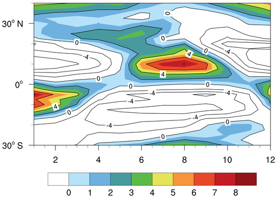
Figure 1.
Latitude–time cross-section of 850 hPa zonal wind (2011–2020) mean along 110°–120° E. The shaded area denotes positive zonal winds (unit: m s−1). The x-axis represents months from January to December.
3. Results
3.1. Predictions of Dynamic and Thermodynamic Variables
To evaluate the model’s prediction skill for the fundamental physical variables during the SCSSM, prediction during the whole monsoon season from May to September is selected. Figure 2 shows the TCC distribution of the zonal winds at 200 hPa and 850 hPa between reanalysis and prediction with different lead times. It can be obtained that CAMS–CSM has a reasonable capability to predict the 200 hPa zonal wind as the TCC reaches mostly above 0.6 for the whole region at lead times of 1–11 days (Figure 2a,b,e,f) and most of the region passes the significance test with a confidence level of 95%. The region with highest capability is generally located in 5°–30° N, which contains the SCS surroundings. The area of (5°–15° N), which is confined by the SCSSM index, is named as “index–limited region” in the following. The prediction capability becomes less proficient with increasing lead times. In addition, the difference between T106 and T106 × T255 is minor at most lead times in the index-limited region (Figures S1–S4). However, the prediction capability of T106 × T255 is significantly higher than that of T106 along Northeast China and south of Lake Balkhash for lead times of 21–31 days. The results of 850 hPa zonal wind indicate the same characteristics as 200 hPa zonal wind. The areas with better prediction capabilities are mainly concentrated in the Arabian Sea, the Bay of Bengal, and the southern part of the SCS. At the same time, the prediction differences demonstrate that T106 × T255 has relatively higher prediction capabilities around Lake Baikal and in the southern part of the index-limited area, while T106 shows a better prediction skill capability on the ocean (Figures S1–S4).
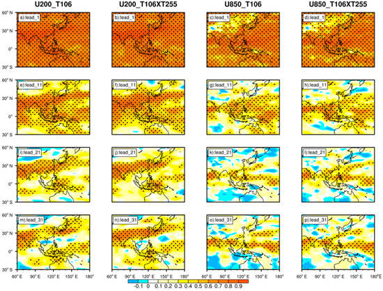
Figure 2.
The TCC distribution (shading) of 200 hPa and 850 hPa zonal wind field between prediction results (T106 and T106 × T255) and reanalysis for different lead times. The values exceeding 95% confidence level according to Student’s t-test are dotted. (a,e,i,m): 200 hPa zonal wind in T106; (b,f,j,n): 200 hPa zonal wind in T106 × T255; (c,g,k,o): 850 hPa zonal wind in T106; and (d,h,l,p): 850 hPa zonal wind in T106 × T255.
On the other hand, the prediction ability for the meridional wind (Figure 3) is not as good as that for zonal wind. At 200 hPa, when it comes to the index-limited region, T106 shows a slightly higher prediction skill than T106 × T255 for lead times of 1–31 days. In the index-limited region of 850 hPa, the prediction results are consistent with that of 200 hPa. The advantage of T106 × T255 over T106 is evident in the eastern and northeastern regions of China and the northwest Pacific. Overall, with the increasing lead times, the prediction deviation of T106 and T106 × T255 is gradually increasing, and the prediction of T106 has a slight advantage in the ocean, while on the land, the prediction capability of T106 × T255 is obviously higher than that of T106.
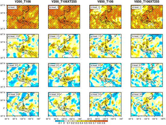
Figure 3.
Same as Figure 2, but for 200 hPa and 850 hPa meridional wind. (a,e,i,m): 200 hPa meridional wind in T106; (b,f,j,n): 200 hPa meridional wind in T106 × T255; (c,g,k,o): 850 hPa meridional wind in T106; and (d,h,l,p): 850 hPa meridional wind in T106 × T255.
The overall prediction capability for θse is reasonable (Figure 4a–h), and the two prediction results are almost consistent. Within the lead time of 11 days, the TCC of most regions is higher than 0.6 and passes the significant test at the confidence level of 95%. The weak prediction capability is mainly restrained in the Philippine Islands and the area to the east. However, the area with weak prediction capability of T106 × T255 is slightly smaller than that of T106. Another prominent feature of the SCSSM onset is the remarkable seasonal enhancement in precipitation intensity [4]. Therefore, the model prediction of precipitation is investigated (Figure 4i–p). The prediction ability for precipitation is conspicuously weaker than the zonal wind and θse, and in some regions, a negative correlation even exists. From Equation (1), θse is closely related to T and q, which are hereafter discussed (Figures S5–S8). The distributions of TCC in T and θse are similar, which indicates that the prediction results of θse may depend primarily on T. At the same time, the weaker prediction ability for q could constrain the prediction of θse, which may further restrict the model’s prediction of SCSSM onset.
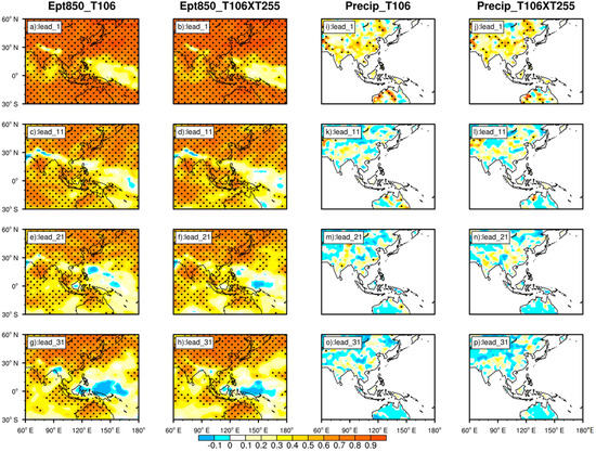
Figure 4.
Same as Figure 2, but for 850 hPa θse (a–h) and precipitation (i–p).
In addition, the evolutions of the pattern correlation coefficient (PCC) of 850 hPa zonal and meridional winds before and after the SCSSM onset are analyzed. Zonal and meridional winds of 850 hPa in the region (20° S–30° N, 60°–150° E) are selected for our study (Figure 5). The PCC prediction for zonal wind is significantly higher than those for meridional wind. With the increasing lead times, the model’s PCC prediction skill gradually decreases. Furthermore, the prediction skill is weak during the adjustment phase of the circulation in late spring and improves significantly after the monsoon onset. Prediction for meridional wind is worse than that for zonal wind, consistent with basic prediction ability for zonal and meridional winds. Finally, attention is paid to the effect of schemes on the predicting ability (Figure 5c,f); no significant difference exists between T106 and T106 × T255.
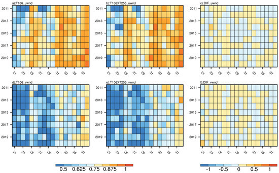
Figure 5.
The pattern correlation coefficients between reanalysis and model predictions of (a,d) T106 and (b,e) T106 × T255 for (a–c) zonal wind and (d–f) meridional wind at 850 hPa over the SCSSM region (20° S–30° N, 60°–150° E) for 2011–2020 (y-axis) from the 21st pentad to the 38th pentad (x-axis) for lead times of 1–31 days. The differences in pattern correlation coefficients in the two models are presented in (c,f).
3.2. Predictions of SCSSM Indices and the Onset Date
The TCC and RMSE are calculated between reanalysis and prediction for seven indices (Table 1) with lead times of 1–31 days. Figure 6 indicates that with increasing lead times, the TCC (RMSE) shows a general decreasing (increasing) trend. From the prediction of TCC for both schemes (Figure 6a,c) within the lead times of 1–31 days except for Li index [32], the TCC of all indices almost passes the significant test with a 95% confidence level. In addition, the model is more proficient for indices defined in a way that the 850 hPa zonal wind is averaged over a region, such as a China Meteorological Administration (CMA) index (black line), the Wang (2004) index [33], and the Jin index [35]. For indices defined with multiple levels and different regions, the prediction capability shows inconsistent results. For the He index [31], the prediction capability is superior from the 1st to the 31st lead day. However, for the Wang (2009) index which involves two regions and two levels [9], the prediction capability is lower than He index for most lead times, especially from the 7th to 13th lead day, indicating that the prediction capability may decrease when the area expands. Concentrating on Li index, it involves different levels of zonal and meridional winds, and the difference between the two levels of divergence is used as the definition of the index. The model itself is weak in predicting the meridional wind, and the calculation error of the divergence may further make the prediction capability of the Li index weaker. Similar results also exist in RMSE (Figure 6b,d). Additionally, when it comes to the difference between the two predictions (Figure 6e,f), the difference between them is from –0.2 to 0.2 for most of the indices in all lead times. Focusing on the Li index, two schemes show more significant deviations. The fluctuation of prediction bias is obvious with different lead times: in lead times of 5–9 days and 13–16 days, the T106 × T255 has better prediction results than T106, but in lead times of 10–12 days and 17–19 days, the T106 exhibits more advantageous performance.
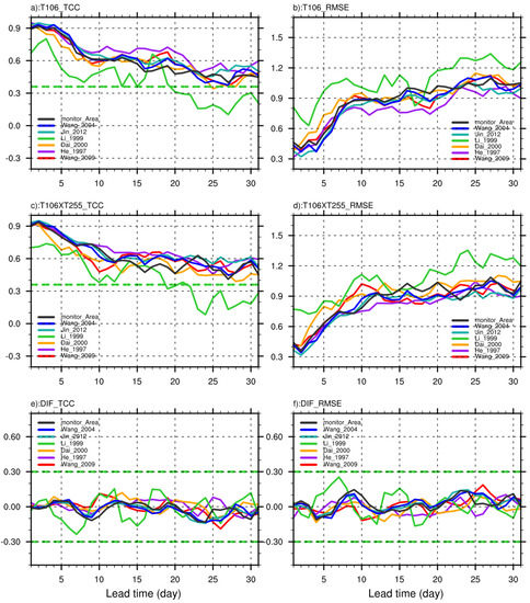
Figure 6.
The TCC and RMSE between prediction and reanalysis, and the difference between two model results for lead times of 1–31 days. (a) TCC between T106 and NCEP2 (b) RMSE between T106 and NCEP2 (c) TCC between T106 × T255 and NCEP2 (d) RMSE between T106 × T255 and NCEP2 (e) TCC difference (f) RMSE difference. The green dotted line in (a,b) is the value (0.36) of the critical correlation coefficient passing the t-test with a confidence level of 99%.
The criteria used to determine the SCSSM onset date is elaborated in Section 2.3. The calculated value (
) between NCEP2 and ERA5 is 0.96, passing the significant test with a 99% confidence level, which indicates that the onset date of SCSSM is consistent despite the use of different reanalysis data. Hence, it is more objective to use this criterion to judge the onset date of the monsoon. When the difference between the predicted and reanalyzed results is larger than two pentads, it is a failed prediction case. The model gives reliable prediction results for SCSSM onset date in most years. The prediction success rate in T106 is 88.89%, while it is 77.78% in T106 × T255.
3.3. Case Study
From 2011 to 2020, 2015 is a special case when the model predicts an unusually early onset. Both NCEP2 and ERA5 show that the onset date of SCSSM is the 34th pentad, compared to the 28th pentad in T106 and 27th pentad in T106 × T255. Furthermore, the pentad-by-pentad evolution of essential variables and the higher- and lower-level circulation backgrounds during the SCSSM onset will be investigated to identify critical factors contributing to the failure of the prediction. Figure 7 illustrates the evolution of zonal wind in T106, T106 × T255, and the reanalysis data (NCEP2 and ERA5) during the SCSSM onset period in 2015. According to the evolution of the zonal wind in T106 (Figure 7a), from the 28th pentad, the westerly wind is mainly controlled over the SCS. Although it is interrupted at the 31st pentad, it recovers quickly at the 33rd pentad. As for the observation results, the westerly wind over the SCS is weak in the 28th pentad and cannot reach the standard of the onset. After that, the westerly wind over the SCS is controlled by the easterly wind until the 34th pentad. The prediction of T106 indicates that the monsoon onset date is the 28th pentad, while it is the 27th of T106 × T255 (Figure 7b).
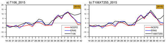
Figure 7.
Pentad-by-pentad evolution of zonal wind averages (y-axis; unit: m.s−1) in the SCSSM monitoring area (5°–15° N, 110°–120° E) for 2015 (for lead times of 1–31 days) from 19th pentad to 42nd pentad (x-axis). Red and blue lines indicate the result of NCEP2 and ERA5, respectively, with the black lines representing the two schemes of T106 (a) and T106 × T255 (b).
From the 21st to the 36th pentad, with reference to the 5°–15° N region, T106 predicts the growth of θse occurring around the 26th pentad (Figure 8b). At the same time, the observations are still relatively stable (Figure 8a). The escalation in the θse is not observed until around the 30th pentad. This suggests that T106 predicts the growth of θse roughly four pentads earlier, which impacts the prediction of SCSSM onset. Moreover, the difference (Figure 8c) shows that a cold bias exists in T106, and it is particularly evident in the pre-onset. On the contrary, T106 × T255 around the 26th pentad also predicts an increase in θse (Figure 8d). Unlike the T106 prediction, a weak thermal bias appears in the T106 × T255 (Figure 8e). However, the difference between the predicted and reanalysis results of θse in T106 × T255 is small (less than 6 K in most regions), while this difference is more pronounced in T106 (more than 12 K in most regions). For example, T106 × T255 can capture θse more reasonably during the SCSSM onset, but the prediction of its evolution process is lacking, contributing to the failure of predicting the onset of SCSSM.
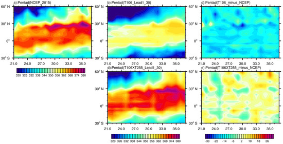
Figure 8.
Latitude–pentad cross–section of 850 hPa mean θse (2015) along 110°–120° E. The shaded area denotes θse values (unit: K). (a): reanalysis; (b,d): prediction; (c,e): difference between prediction and reanalysis.
Concerning the circulation case of T106 (Figure 9), pentad 0 is the onset date in the reanalysis data (34th pentad, 2015). The observed results show a clear weakening trend in the WPSH in the east during the onset of SCSSM (32nd–34th pentad). The observed WPSH is significantly weaker than predicted on the 34th pentad. From the 32nd to 34th pentad, the observed results manifest a more apparent negative anomaly in the Bay of Bengal area, corresponding to the formation and deepening development of the Bay of Bengal trough. The southwestern airflow in front of the trough travels eastward and accelerates to the SCS. From the beginning of the 33rd pentad, the observations display a more pronounced “vortex pair” near the equator (80° E), followed by the onset of SCSSM, but the model fails to capture this critical signal. From the beginning of the onset pentad (34th pentad), an obvious easterly wind anomaly appears along the Bay of Bengal, which means that the model fails to reasonably predict the strengthening of the westerly wind. Meanwhile, the observed intensity of WPSH is much weaker than that of predictions, corresponding to the fact that the onset of SCSSM is earlier in the prediction, which has finished the weakening and eastern withdrawal of WPSH. Similar results can be found in T106 × T255 (Figure 10). By comparing the predicted results of the two schemes, the prediction of the SCSSM onset date is significantly earlier for both models at the same lead time, but the prediction of the WPSH intensity in T106 is more potent than that of T106 × T255 before and after the SCSSM onset. In other words, the prediction of T106 for the WPSH intensity is more deviated from the actual situation during the onset.
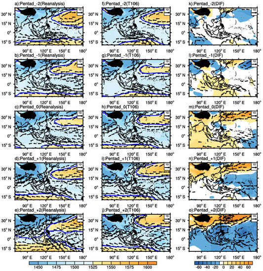
Figure 9.
The mean wind (vector; unit: m.s−1) and hgt (shading; unit: gpm) at 850 hPa for 2015 with earlier predictions of T106. (a–e): reanalysis; (f–j): prediction, (k–o): difference between predictions and reanalysis. Pentad_0 illustrates the onset date based on reanalysis; Pentad_+ (−)1,2 states the pentad later (earlier) than Pentad_0 for one or two pentads. Only wind with speed of above 5 m s−1 is plotted. The blue contour of 1520 gpm denotes the WPSH.
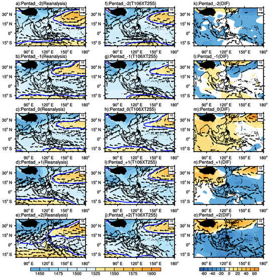
Figure 10.
Same as Figure 9, but for T106 × T255 forecasts. (a–e): reanalysis; (f–j): prediction; (k–o): difference between predictions and reanalysis.
For the higher-level troposphere, the SAH shifted northward from the 32nd to the 33rd pentad. Its intensity increased, and the jet stream was significantly enhanced on both sides (Figure 11a–c). In the prediction of T106, the main body of SAH is northward and weaker, and it is on the northwest side of the Indochina Peninsula. Starting from the 33rd pentad (Figure 11g), the SAH has a breaking trend and breaks at the 34th pentad (Figure 11h). Compared with the observed results: a negative anomaly exists, and the cyclonic anomaly is prominent (Figure 11k–o), which means that CAMS–CSM could not reasonably capture the intensification of SAH in 2015. Concerning the location of the SAH, it is speculated that the SAH may have completed its advance to the northwest in the predicted results of T106, i.e., the SCSSM has already erupted in T106. In the predicted results of T106 × T255 (Figure 12), the overall prediction results are similar to those of T106, with a more reasonable prediction of SAH intensity and smaller deviation in the wind field than T106 (Figure 12k–o).
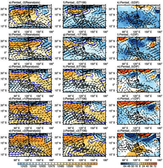
Figure 11.
Same as Figure 9, but for 200 hPa. The blue contour of 12,480 gpm denotes SAH. (a–e): reanalysis; (f–j): prediction; (k–o): difference between predictions and reanalysis.
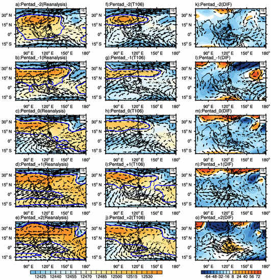
Figure 12.
Same as Figure 11, but for T106 × T255 forecasts. (a–e): reanalysis; (f–j): prediction; (k–o): difference between predictions and reanalysis.
4. Conclusions and Discussion
The South China Sea summer monsoon (SCSSM) is closely related to the rain belt in East Asia. Skillful predictions of SCSSM play essential roles in regional disaster preventions and mitigations. Based on multiple observational datasets, the 1–31-day predictions of SCSSM based on the Chinese Academy of Meteorological Sciences climate system model (CAMS–CSM) climate forecast system are examined and diagnosed with two schemes of T106 and T106 × T255 (with a nudging process added) for the retrospective forecast experiment from 2011 to 2020. The SCSSM indices, onset and associated dynamic and thermodynamic characteristics are analyzed with the following conclusions obtained.
The essential SCSSM elements such as the zonal wind, temperature, humidity and θse at the lower levels are mostly predicted with generally reasonable capability for lead times of <11 days, but the prediction ability decreased during the subseasonal scale, in agreement with previous studies [25,41]. However, the model shows relatively lower skills for predictions of meridional winds and precipitation. Therefore, among the selected seven SCSSM indices, the model shows higher skills for those defined by zonal winds, while it could not perform well for the indices involving both meridional and zonal winds over different regions.
Assessments also indicate that the prediction skills tend to decrease with the increasing lead times. The T106 × T255 model with nudging process shows advantages over the continent, while over the ocean, the standalone T106 is characterized by a slight superiority. Furthermore, the prediction skill is relatively weak during the circulation adjustment period before the monsoon onset, while a significant enhancement occurs after that.
Generally, the models are capable of predicting the SCSSM onset and capturing the essential signals for most years during the retrospective forecast experiment, in which the year of 2015 is taken as an example of prediction failure for further investigations. Large-scale environmental factors impacting SCSSM onset during 2015 were discussed. In the 2015 case, the shift in zonal wind and the increase in θse are not well reflected in the model predictions, suggesting that the model fails to accurately predict changes in dynamic and thermodynamic conditions that are closely linked to the SCSSM onset [8,33]. Accordingly, biases for the large-scale circulation field are mainly concentrated on prediction deficiencies of both upper-level intensification and northward movement processes of SAH and lower-level elements, including the weakening and eastward withdrawal of the WPSH, the appearance of “vortex pairs” near the equator and the acceleration of the westerly wind [8,9,10]. The model fails to reasonably capture the precursor signal of SCSSM onset which further leads to the failure of predicting onset date.
The numerical model predictions are always characterized by relatively less-proficient performances on the subseasonal timescale due to significant impacts from both initial conditions and boundary forcings [40]. In this study, the 1–31-day predictions of the SCSSM are discussed towards the CAMS–CSM climate forecast system with different schemes of T106 and T106 × T255 at the same resolution. Although the nudging process in T106×T255 could partly improve the prediction skills over specific areas, various deficiencies can still be found in the model. Further investigations would be focused on the features of finer-resolution model predictions and possible improvements via advanced postprocessing procedures [42,43]. In addition, experiments covering a longer period would also be carried out to reveal more characteristics of the subseasonal forecasts.
Supplementary Materials
The following supporting information can be downloaded at: https://www.mdpi.com/article/10.3390/atmos13071051/s1, Figure S1: The TCC difference (T106 minus T106 × T255) between prediction results (T106 and T106 × T255) and reanalysis (NCEP2) (shade) of 200 hPa zonal wind; the areas exceeding 95% confidence level according to Student’s t-test are dotted. The black box represents the area limited by SCSSM onset index (5–15° N, 110–120° E). (a–d) represent the results of different lead times (1–31 days), respectively; Figure S2. Same as Figure S1 but for 850 hPa zonal wind; Figure S3: Same as Figure S1 but for 200 hPa meridional wind; Figure S4: Same as Figure S1 but for 850 hPa meridional wind; Figure S5. The TCC distribution between prediction results (T106) and reanalysis results (NCEP2) (shade) of 850 hPa T; the areas exceeding 95% confidence level according to Student’s t-test are dotted. The black box represents the area limited by SCSSM onset index (5–15° N, 110–120° E). (a–d) represent the results of different lead times, respectively; Figure S6: Same as Figure S5 but for 850 hPa T in T106 × T255; Figure S7: Same as Figure S5 but for 850 hPa q in T106; Figure S8: Same as Figure S5 but for 850 hPa-specific q in T106 × T255.
Author Contributions
All authors equally collaborated in the research presented in this publication by making the following contributions. Conceptualization, Y.F.; Data curation, L.W.; Formal analysis, X.W.; Investigation, X.W.; Methodology, Y.F., L.W. and Y.Z.; Supervision, Y.F.; Writing—original draft, X.W.; Writing—review and editing, Y.F., L.W. and Y.Z. All authors have read and agreed to the published version of the manuscript.
Funding
This research was jointly supported by the National Key Research and Development Program of China 2019YFC1510004, the National Natural Science Foundation of China (Grants 42105030; 42005015), the Natural Science Foundation of the Jiangsu Higher Education Institutions of China 21KJB170005 and the College Students’ Practice Innovation Training Program of Jiangsu Province, NUIST Students’ Platform for Innovation and Entrepreneurship Training Program (202210300005Z).
Institutional Review Board Statement
Not applicable.
Informed Consent Statement
Not applicable.
Data Availability Statement
The observation data in this paper are publicly available. These data can be found here: https://psl.noaa.gov/data/gridded/data.ncep.reanalysis2.html; https://cds.climate.copernicus.eu/cdsapp#!/dataset/reanalysis–era5–pressure–levels?tab=form (accessed on 5 April 2022). The original data supporting the conclusions will be provided by the authors without reservation.
Acknowledgments
We are thankful for the support from the Startup Foundation for Introducing Talent of NUIST.
Conflicts of Interest
The authors declare no conflict of interest.
References
- Ding, Y. Summer Monsoon Rainfalls in China. J. Meteorol. Soc. Jpn. Ser. II 1992, 70, 373–396. [Google Scholar] [CrossRef] [Green Version]
- Kong, W.; Chiang, J.C.H. Interaction of the Westerlies with the Tibetan Plateau in Determining the Mei-Yu Termination. J. Clim. 2020, 33, 339–363. [Google Scholar] [CrossRef] [Green Version]
- Tao, S.; Chen, L. A review of recent research of the east Asian summer monsoon in China. In Monsoon Meteorology; Chang, C.-P., Krishnamurti, T.N., Eds.; Oxford University Press: New York, NY, USA, 1987; pp. 60–92. [Google Scholar]
- Ding, Y.; Chan, J. The East Asian Summer Monsoon: An Overview. Meteorol. Atmos. Phys. 2005, 89, 117–142. [Google Scholar] [CrossRef]
- Ding, Y.; Liu, Y. Onset and the evolution of the Summer Monsoon over the South China Sea during SCSMEX Field Experiment in 1998. J. Meteorol. Soc. Jpn. Ser. II 1999, 79, 255–276. [Google Scholar] [CrossRef] [Green Version]
- Huang, R.H.; Xu, Y.; Wang, P.; Zhou, L. The features of the catastrophic flood over the Changjiang River Basin during the summer of 1998 and cause exploration. Clim. Environ. Res. 1998, 3, 300–313. (In Chinese) [Google Scholar] [CrossRef]
- Shao, X.; Huang, P.; Huang, R. A review of the South China Sea summer monsoon onset. Adv. Earth Sci. 2014, 29, 1126–1137. (In Chinese) [Google Scholar] [CrossRef]
- He, J.; Wen, M.; Shi, X.; Zhao, Q. Splitting and eastward withdrawal of the subtropical high belt during the onset of the South China Sea summer monsoon and their possible mechanism. J. Nanjing Univ. Nat. Sci. Ed. 2002, 38, 318–330. (In Chinese) [Google Scholar]
- Wang, B.; Huang, F.; Wu, Z.; Yang, J.; Fu, X.; Kikuchi, K. Multi-Scale Climate Variability of the South China Sea Monsoon: A Review. Dyn. Atmos. Ocean. 2009, 47, 15–37. [Google Scholar] [CrossRef]
- Liu, B.; Zhu, C. A Possible Precursor of the South China Sea Summer Monsoon Onset: Effect of the South Asian High: SAH Leads the Onset of the SCSSM. Geophys. Res. Lett. 2016, 43, 11072–11079. [Google Scholar] [CrossRef]
- Li, C.; Yanai, M. The Onset and Interannual Variability of the Asian Summer Monsoon in Relation to Land–Sea Thermal Contrast. J. Clim. 1996, 9, 358–375. [Google Scholar] [CrossRef] [Green Version]
- Wu, R.; Wang, B. Interannual Variability of Summer Monsoon Onset over the Western North Pacific and the Underlying Processes. J. Clim. 2000, 13, 2483–2501. [Google Scholar] [CrossRef]
- Wang, B.; Wu, R.; Lau, K.-M. Interannual Variability of the Asian Summer Monsoon: Contrasts between the Indian and the Western North Pacific–East Asian Monsoons. J. Clim. 2001, 14, 4073–4090. [Google Scholar] [CrossRef]
- Kwon, M.; Jhun, J.; Wang, B.; An, S.; Kug, J. Decadal Change in Relationship between East Asian and WNP Summer Monsoons. Geophys. Res. Lett. 2005, 32, L16709. [Google Scholar] [CrossRef] [Green Version]
- Krishnamurti, T. Summer Monsoon Experiment—A Review. Mon. Weather Rev. 1985, 113, 1590–1626. [Google Scholar] [CrossRef] [Green Version]
- Murakami, T. Empirical Orthogonal Function Analysis of Satellite-Observed Outgoing Longwave Radiation During Summer. Mon. Weather Rev. 1980, 108, 205–222. [Google Scholar] [CrossRef] [Green Version]
- Wu, G.; Zhang, Y. Tibetan Plateau Forcing and the Timing of the Monsoon Onset over South Asia and the South China Sea. Mon. Weather Rev. 1998, 126, 913–927. [Google Scholar] [CrossRef]
- Huang, R.; Sun, F. Impacts of the thermal state and the convective activities in the tropical western warm pool on the summer climate anomalies in East Asia. Chin. J. Atmos. Sci. 1994, 18, 141–151. (In Chinese) [Google Scholar]
- Huang, R.; Sun, F. Impact of the convective activities over the western Tropical Pacific warm pool on the intraseasonal variability of the East Asian summer monsoon. Chin. J. Atmos. Sci. 1994, 18, 456–465. (In Chinese) [Google Scholar]
- Wu, G.; Liu, Y.; He, B.; Bao, Q.; Duan, A.; Jin, F.-F. Thermal Controls on the Asian Summer Monsoon. Sci. Rep. 2012, 2, 404. [Google Scholar] [CrossRef] [Green Version]
- Huang, R.; Chen, J.; Wang, L.; Lin, Z. Characteristics, Processes, and Causes of the Spatio-Temporal Variabilities of the East Asian Monsoon System. Adv. Atmos. Sci. 2012, 29, 910–942. [Google Scholar] [CrossRef]
- Fan, Y.; Fan, K.; Xu, Z.; Li, S. ENSO–South China Sea Summer Monsoon Interaction Modulated by the Atlantic Multidecadal Oscillation. J. Clim. 2018, 31, 3061–3076. [Google Scholar] [CrossRef]
- You, J.; Jian, M.; Gao, S.; Cai, J. Interdecadal Change of the Winter-Spring Tropospheric Temperature Over Asia and its Impact on the South China Sea Summer Monsoon Onset. Front. Earth Sci. 2021, 8, 661–675. [Google Scholar] [CrossRef]
- Vitart, F.; Ardilouze, C.; Bonet, A.; Brookshaw, A.; Chen, M.; Codorean, C.; Déqué, M.; Ferranti, L.; Fucile, E.; Fuentes, M.; et al. The Subseasonal to Seasonal (S2S) Prediction Project Database. Bull. Am. Meteorol. Soc. 2017, 98, 163–173. [Google Scholar] [CrossRef]
- Li, Q.; Yang, S.; Wu, T.; Liu, X. Subseasonal Dynamical Prediction of East Asian Cold Surges. Weather Forecast. 2017, 32, 1675–1694. [Google Scholar] [CrossRef]
- Brunet, G.; Shapiro, M.; Hoskins, B.; Moncrieff, M.; Dole, R.; Kiladis, G.N.; Kirtman, B.; Lorenc, A.; Mills, B.; Morss, R.; et al. Collaboration of the Weather and Climate Communities to Advance Subseasonal-to-Seasonal Prediction. Bull. Am. Meteorol. Soc. 2010, 91, 1397–1406. [Google Scholar] [CrossRef]
- Rong, X.; Li, J.; Chen, H.; Xin, Y.; Su, J.; Hua, L.; Zhou, T.; Qi, Y.; Zhang, Z.; Zhang, G.; et al. The CAMS Climate System Model and a BasicEvaluation of Its Climatology and Climate Variability Simulation. J. Meteorol. Res. 2018, 32, 839–861. [Google Scholar] [CrossRef]
- Liu, B.; Su, J.; Ma, L.; Tang, Y.; Rong, X.; Li, J.; Chen, H.; Liu, B.; Hua, L.; Wu, R. Seasonal Prediction Skills in the CAMS-CSM Climate Forecast System. Clim. Dyn. 2021, 57, 2953–2970. [Google Scholar] [CrossRef]
- Kanamitsu, M.; Ebisuzaki, W.; Woollen, J.; Yang, S.-K.; Hnilo, J.J.; Fiorino, M.; Potter, G.L. NCEP–DOE AMIP-II Reanalysis (R-2). Bull. Am. Meteorol. Soc. 2002, 83, 1631–1644. [Google Scholar] [CrossRef]
- Hersbach, H.; Bell, B.; Berrisford, P.; Hirahara, S.; Horányi, A.; Muñoz-Sabater, J.; Nicolas, J.; Peubey, C.; Radu, R.; Schepers, D.; et al. The ERA5 Global Reanalysis. Q. J. R. Meteorol. Soc. 2020, 146, 1999–2049. [Google Scholar] [CrossRef]
- He, M. Summer monsoon and Yangtze River basin precipitation (Abstract). In Preprint of Abstracts of Papers for the First WNO International Workshop on Monsoon Studies; WMO: Geneva, Switzerland, 1997; Volume 786, pp. 67–67B. [Google Scholar]
- Li, C.; Zhang, L. Summer monsoon activities in the South China Sea and its impacts. Chin. J. Atmos. Sci. 1999, 23, 257–266. [Google Scholar] [CrossRef]
- Wang, B.; Lin, H.; Zhang, Y.; Lu, M.-M. Definition of South China Sea Monsoon Onset and Commencement of the East Asia Summer Monsoon. J. Clim. 2004, 17, 699–710. [Google Scholar] [CrossRef] [Green Version]
- Dai, N.; Xie, A.; Zhang, Y. Interannual and interdecadal variations of summer monsoon activities over South China Sea. Clim. Environ. Res. 2000, 5, 363–374. [Google Scholar]
- Jin, L.; Zhao, P. Observational and modeling studies of impacts of the South China Sea monsoon on the monsoon rainfall in the middle-lower reaches of the Yangtze River during summer. Acta Meteorol. Sin. 2012, 26, 176–188. [Google Scholar] [CrossRef]
- Xie, A.; Liu, X.; Ye, Q. Equatorial vortex and the onset of summer monsoon over the South China Sea. Acta Meteorol. Sin. 1997, 55, 611–619. (In Chinese) [Google Scholar]
- Li, J.; Zhang, L. Wind Onset and Withdrawal of Asian Summer Monsoon and Their Simulated Performance in AMIP Models. Clim. Dyn. 2009, 32, 935–968. [Google Scholar] [CrossRef]
- Wang, Q.; Ding, Y. Climatological aspects of evolution of summer monsoon over the northern South China Sea. Acta Meteorol. Sin. 1997, 55, 466–483. [Google Scholar]
- Huangfu, J.; Huang, R.; Chen, W. Relationship between the South China Sea Summer Monsoon Onset and Tropical Cyclone Genesis over the Western North Pacific. Int. J. Climatol. 2017, 37, 5206–5210. [Google Scholar] [CrossRef]
- Zhu, Z.; Li, T. Empirical Prediction of the Onset Dates of South China Sea Summer Monsoon. Clim. Dyn. 2017, 48, 1633–1645. [Google Scholar] [CrossRef]
- Liu, B.; Zhu, C. Subseasonal-to-Seasonal Predictability of Onset Dates of South China Sea Summer Monsoon: A Perspective of Meridional Temperature Gradient. J. Clim. 2021, 34, 5601–5616. [Google Scholar] [CrossRef]
- Xu, J.; Koldunov, N.; Remedio, A.R.C.; Sein, D.V.; Zhi, X.; Jiang, X.; Xu, M.; Zhu, X.; Fraedrich, K.; Jacob, D. On the Role of Horizontal Resolution over the Tibetan Plateau in the REMO Regional Climate Model. Clim. Dyn. 2018, 51, 4525–4542. [Google Scholar] [CrossRef] [Green Version]
- Zhu, S.; Zhi, X.; Ge, F.; Fan, Y.; Zhang, L.; Gao, J. Subseasonal forecast of surface air temperature using superensemble approaches: Experiments over Northeast Asia for 2018. Weather Forecast. 2021, 36, 39–51. [Google Scholar] [CrossRef]
Publisher’s Note: MDPI stays neutral with regard to jurisdictional claims in published maps and institutional affiliations. |
© 2022 by the authors. Licensee MDPI, Basel, Switzerland. This article is an open access article distributed under the terms and conditions of the Creative Commons Attribution (CC BY) license (https://creativecommons.org/licenses/by/4.0/).