Abstract
Regional climate projections are widely used in impact studies such as adaptations in agronomy. The big challenge of the climate modeling community is to serve valuable instructions regarding the reliability of these simulations to encourage agronomists to use this kind of information properly. The study validates 15 high-resolution ensembles from the Coordinated Regional Climate Downscaling Experiment-European Domain (EURO-CORDEX) for maximum temperature, minimum temperature, and precipitation to fulfill this task. Three evaluation metrics are calculated (mean absolute error, root mean square error, and correlation) for the means and the 5th and 95th percentiles. The analyses are elaborated for annual and monthly means and the vegetation periods of maize and winter wheat. Only arable lands are considered to exclude the effects of the topography. Furthermore, an ensemble selection is applied based on the evaluation metrics to reduce the data use. The five models with the best performance in the case of winter wheat are CNRM-CM5-CLMcom-CCLM4-8-17_v1, MOHC-HadGEM2-ES-IPSL-WRF381P_v1, MOHC-HadGEM2-ES-KNMI-RACMO22E_v2, MOHC-HadGEM2-ES-CLMcom-CCLM4-8-17_v1, and MPI-M-MPI-ESM-LR-KNMI-RACMO22E_v1. In the case of the vegetation period of maize, the models with the best skills are MPI-M-MPI-ESM-LR-KNMI-RACMO22E_v1, CNRM-CM5-IPSL-WRF381P_v2, MPI-M-MPI-ESM-LR-SMHI-RCA4_v1a, MOHC-HadGEM2-ES-IPSL-WRF381P_v1, and MOHC-HadGEM2-ES-KNMI-RACMO22E_v2. Quantifying the errors in climate simulations against observations and elaborating a selection procedure, we developed a consistent ensemble of high time and space resolution climate projections for agricultural use in Romania.
1. Introduction
The IPCC has reported that the observed climate change is already affecting agriculture and the food security sector through increasing temperatures, changing precipitation patterns, and greater frequency of extreme weather events [1]. Furthermore, at the European level, in the Post-2020 Common Agriculture Policy, three of the policy’s nine “specific objectives” will focus on the environment and climate, and one of them aims to contribute to climate change mitigation and adaptation [2,3,4]. Studies on the assessment of the climate change impact on land suitability require high-quality climate information.
In current climate research, climate modeling represents the primary tool for analyzing the climate system’s response to natural and anthropogenic forcing, and thus for projecting the future climate. Global Climate Models (GCMs) provide reliable information on global and large regional scales, covering a vast and very different landscape with potential for various climate-correlated extreme events. However, the horizontal resolution of GCMs, which typically ranges from 250 to 600 km, limits the possibility of addressing smaller-scale processes. Regional Climate Models (RCMs), with a higher spatial resolution (up to 11 km) over a limited area driven by GCMs, provide more appropriate climate information on such smaller scales. Therefore, the impact and adaptation measures can be more reliable. In time, the use of RCMs has grown, their resolution has increased, documentation has developed, new components have been added, and various ensemble experiments have become more widespread [5]. The EURO-CORDEX project is a coordinated initiative to produce a more robust assessment of climate change projections over the European region [6].
Global and regional climate model projections present significant uncertainties, primarily due to issues of scale resolution, leading to incoherencies among the models [7]. For this reason, many studies use the outputs of multiple future climate projections to increase confidence [7,8,9,10]. This approach leads to large data sets to be processed and analyzed. Based on the data availability, resolution, and confidence in the model’s performance, some scholars choose to consider only one model or a small number of models in their analysis [11,12,13,14]. Under these circumstances, our paper aims to select a reasonable number of ensembles, but still keep the most important climate characteristics to estimate further agro-climatological conditions for impact studies. However, numerous studies have focused on validating EURO-CORDEX against observational time series [15,16,17,18,19,20]. Beyond these works, in this study, the skills of the regional climate models are quantified not only for the widely used periods (e.g., annual, seasonal) but for vegetation periods of two cereal crops.
This paper is part of a larger project, AGROCLIMRO (www.agroclim.ro, accessed on 1 July 2021), aiming at re-zoning the agroclimatic suitability areas in Romania for the two most-extended crops in the country, maize and winter wheat. It is in line with the Common Agricultural Policy and European Union Adaptation Strategy that suggests that each member state delineates the suitability for crop growth. At the same time, this topic fits very well to flagship question 1 of the Pannonian Basin Experiment Project (PannEx) [21].
This paper aims to present the methodology and results for choosing among many RCMs running under different driving models which best fit the specified crops in the focus area. However, the results are valid for Romania and agricultural land in the entire Pannonian Basin.
2. Materials and Methods
2.1. Data Used
Temperature and precipitation are the essential variables for different crops, especially for maize and winter wheat, the dominant ones in Romania. Thus, for validation we considered extreme daily temperatures (maximum and minimum) and daily amount of precipitation in this study.
The analysis was performed based on gridded data at the best spatial resolution available at this moment, 0.1° latitude × 0.1° longitude (~11 × 11 km).
As a reference, we used data from the national ROCADA gridded database developed by the Romanian National Meteorological Administration network [22]. It was chosen as it seems to return the smallest errors for average values against observations compared to other databases at the same spatial resolution covering the focus region, such E-OBS [23,24] or CarpatClim [25,26]. The ROCADA database was derived by interpolating 155 observation points (weather stations) for air temperature and 188 points for precipitation, compared to no more than 31 used for the other databases. Its original datasets are freely available online on PANGAEA [27]. Romania’s territory is covered by 3046 pixels (Figure 1) and has a temporal extension over a 53-year period (1961–2013). For this study, we considered the common period with historical data available of the RCMs: 1971–2000.
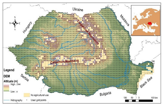
Figure 1.
Grid network used for data analysis.
In terms of modeled data, we used the high-resolution EURO-CORDEX [28] simulations, similar to the observation-derived gridded data. First, we identified all RCMs having daily minimum and maximum air temperature outputs and daily precipitation for each historical experiment and RCP 4.5 and RCP 8.5 (the latter ones are not included in the present study). Since we identified 15 combinations of driving experiments and RCMs (Table 1) and working with them could be time-consuming, we needed to make a hierarchy for all these models. To choose the most appropriate ones for further analysis, they were selected based on their best performance fit for the two crops’ vegetation seasons.

Table 1.
Modeled data features.
2.2. Methods Used
2.2.1. Evaluation Metrics for Validation
Three metrics were calculated between modeled and observation-derived datasets to evaluate regional climate simulations. The procedure was possible since both modeled and observation-derived historical data had the same horizontal resolution. The evaluation was elaborated based on multiannual means between each grid point. The evaluation metrics are the followings:
- i.
- Mean absolute error (MAE) was used to calculate the absolute value of the difference between modeled and observed data (Equation (1)):where is the modeled value; is the observation-derived value; n is the number of grids.
- ii.
- Root mean squared error (RMSE) detects the effect of the outliers in the difference between modeled and observation-derived values (Equation (2))where is the modeled value; is the observation-derived value; n is the number of grids.
- iii.
- Pearson’s Correlation Coefficient (Corr) helped to measure the linear correlation between modeled and observation-derived values.
The metrics were calculated for multiannual means and the 5th and 95th percentile values of the chosen variables to analyze the ability of the models to represent the extreme values.
2.2.2. Algorithm for RCMs Ranking
The ranking of the 15 RCMs considered was developed in 4 steps, as follows:
Step 1. Based on the 3 validation metrics (MAE, RMSE, Corr), a d performance score was assigned to simulations in the case of the variables tasmax, tasmax 95th percentile, tasmin, tasmin 5th percentile, pr, and pr 95th percentile (Table S2). The scoring procedure is adapted after Bartok et al., 2019 [29]. The scores are calculated as described in Equation (3) for MAE and RMSE and Equation (4) for Corr.
where d is the performance score, the closer d is to 1, the better the simulation performs compared to the others; max(X) and min(X) are the maximum and minimum values of the given performance metrics among the 15 models.
Step 2. The d performance scores for each variable and evaluation metric were turned into an initial ranking between 1 and 15 (positionn) since we have 15 models. The highest d score (the model that best fit the observation-derived data) was assigned to 1 (position1 in the ranking), and the lowest d score (the model with the lowest performance against the observation-derived data) was assigned to 15 (position15 in the hierarchy). In this way, a uniform initial ranking was obtained (instead of the relative d performance scores, which vary among variables and metrics).
Step 3. The initial ranking (1 to 15) was converted into a weighted scale to assign values with different orders of magnitude for various positions. In this way, the final step summing up of weights is relevant, where models performing mostly well will have a score much higher than the models performing relatively weakly. The weighted ranking is elaborated based on a non-linear series which starts at 3 (1st initial position receives the value of 3) and is growing as presented in Equation (5):
where xn—the weighted rank of the model on a given position; xn−1 is the weighted rank obtained by the model on the previous position; positionn is the number of the position in the initial ranking (e.g., an xn score of 9 is assigned to the model ranked in position 2 in the initial order: 3 + 2 × 3, where 3 is the rank for the model in position 1 in the initial ranking, 2 is the position of the model for which the weighted rank is calculated; similarly, a score of 18 is assigned to the model ranked in position 3 in the initial ranking (9 + 3 × 3), etc.). The series was introduced in reverse order to set the highest value (360) to the highest initial position (rank1).
The score was calculated for each model and each metric (see Table S3 for annual and vegetation periods in Supplementary material).
Step 4. We developed the final ranking of the models based on a final score (FS) obtained by summing up the weighted ranks calculated in Step 3 for each variable and evaluation metric. The higher the final score, the better the simulation performs compared to the others. Since temperature and precipitation act differently on cereal crops, for the final score, we applied weight for the three climatic parameters as follows: tasmin—40%; tasmax—30%, and pr—30% (Equation (6)).
- xn tasminMAE—weighted rank obtained by the model n for tasmin for the MAE metric;
- xn tasminRMSE—weighted rank obtained by the model n for tasmin for the RMSR metric;
- xn tasminCorr—weighted rank obtained by the model n for tasmin for the Pearson Correlation metric;
- xn tasmin5pMAE—weighted rank obtained by the model n for 5th percentile of tasmin for the MAE metric;
- xn tasmin5pRMSE—weighted rank obtained by the model n for 5th percentile of tasmin for the RMSR metric;
- xn tasmin5pCorr—weighted rank obtained by the model n for 5th percentile of tasmin for the Pearson Correlation metric;
- xn tasmaxMAE—weighted rank obtained by the model n for tasmax for the MAE metric;
- xn tasmaxRMSE—weighted rank obtained by the model n for tasmax for the RMSR metric;
- xn tasmaxCorr—weighted rank obtained by the model n for tasmax for the Pearson Correlation metric;
- xn tasmax95pMAE—weighted rank obtained by the model n for 95th percentile of tasmax for the MAE metric;
- xn tasmax95pRMSE—weighted rank obtained by the model n for 95th percentile of tasmax for the RMSR metric;
- xn tasmax95pCorr—weighted rank obtained by the model n for 95th percentile of tasmax for the Pearson Correlation metric;
- xn prMAE—weighted rank obtained by the model n for pr for the MAE metric;
- xn prRMSE—weighted rank obtained by the model n for pr for the RMSR metric;
- xn prCorr—weighted rank obtained by the model n for pr for the Pearson Correlation metric;
- xn pr95pMAE—weighted rank obtained by the model n for 95th percentile of pr for the MAE metric;
- xn pr95pRMSE—weighted rank obtained by the model n for 95th percentile of pr for the RMSR metric;
- xn pr95pCorr—weighted rank obtained by the model n for 95th percentile of pr for the Pearson Correlation metric;
We granted the highest weights to tasmin as it is crucial for plant development and large area crops (such as cereals). It can severely impact the yields by shortening the growing season length and diminishing the growing degree days. Sometimes, it may lead to the incomplete maturity of the plant. Maximum temperature and precipitation received the same weight, 30%, as in the temperate regions; maximum temperature is usually not so high as to endanger the crops as in the Mediterranean or tropical climates. They do not last for many consecutive days when they occur, whereas precipitation can be successfully supplied by irrigation (ground water availability is not a problem in Romania). As the performance of the models differs with the season, the ranking was developed separately for monthly and annual means as well as for the vegetation periods of maize (April–October) and winter wheat (October–June) (Table 3).
2.2.3. Area Analysis
To increase the accuracy of the analysis, we considered only the arable lands for validation. Land use data were updated for 2020, and they were provided by the Agency for Payments and Interventions in Agriculture in Romania (http://www.apia.org.ro/, accessed on 1 July 2021). From the total number of 3046 pixels covering the entire country, after excluding the non-arable land, we retained only 2726 grids, representing 89.5% of the country territory. The selection of grids was made even where a very small arable land is included; for this reason, the number of remaining grids is still relatively high. Even though this decrease does not seem so important, it should be mentioned that the area excluded is from the complex topography regions (high hills and mountains), which usually impose the most important biases. We consider that accuracy for this validation is the best possible, based on the available data at present.
3. Results
3.1. Model Performance on Temperature
First, we compared the multiannual monthly averages of daily tasmax and tasmin derived from the 15 EURO-CORDEX ensembles with the values of the same grid point from the ROCADA database.
The validation metrics for individual models over the 12 months are presented in Figure 2, and the detailed results are included in Supplementary Material as Table S1. The multimodel mean of MAE is 1.3 °C for tasmax and 1.5 °C for tasmin (Table 1). However, there is a wide spread among the models (upper left and bottom left graphs in Figure 2), mainly during the spring and summer. The most significant mean errors are detected for M5, M3, and M7. The difference between RMSE and MAE highlights outliers in errors (in RMSE, the errors are squared before averaging). Larger outliers are detected in January, February, and March, particularly M4, M6, and M11 simulations (upper right and bottom right graphs in Figure 2).
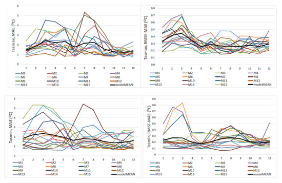
Figure 2.
Validation metrics for tasmax (upper left and right) and tasmin (bottom left and right), EURO-CORDEX simulations (full name of individual models are given in Table 1) against ROCADA observation-derived datasets, over the period 1971–2000.
Focusing on the vegetation periods of maize (April–October) and winter wheat (October–June), in the case of tasmax, the multimodel mean of MAE is 1.40 °C and 1.44 °C, and 1.47 °C and 1.62 °C in case of tasmin, respectively (Table 2).

Table 2.
Validation metrics for tasmax, tasmin, and pr: multimodel mean of 15 EURO-CORDEX simulations against ROCADA observation-derived datasets, over the period 1971–2000.
The overall performance of the models for the two vegetation periods is also analyzed by using the Taylor diagrams. The best fit characterized the maize vegetation period with lower RMSE and standard deviation and stronger spatial correlation (Figure 3).
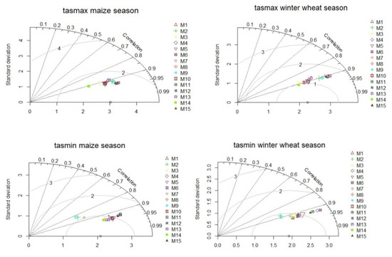
Figure 3.
Validation of tasmax and tasmin for 15 EURO-CORDEX simulations against ROCADA observation-derived datasets over the period 1971–2000 (full names of the individual model are given in Table 1) for vegetation periods of maize (April–October) and winter wheat (October–June). In the diagram, the circle on the Ox-axis represents the observation, and the colored plots represent the different models. Three statistics determine the relative places of the models: the Pearson correlation coefficient (curved axes), the centered RMS error (grey contours), and the standard deviation (Oy-axis). The model fitting best with observations will lie the nearest to the Ox-axis.
MAE and RMSE of the 5th and 95th percentiles were calculated to analyze the performance of the models in representing extreme values. Figure 4 depicts the spread of the models in terms of MAE by months. The larger errors were detected for the 5th percentile for tasmin. M3, M7, and M5 simulations indicated the most significant errors in representing low temperature (upper right graph in Figure 4). The spread among the models in the case of high extremes is smaller. Some outliers are also present, namely, M8 and M9 (lower graphs in Figure 4).
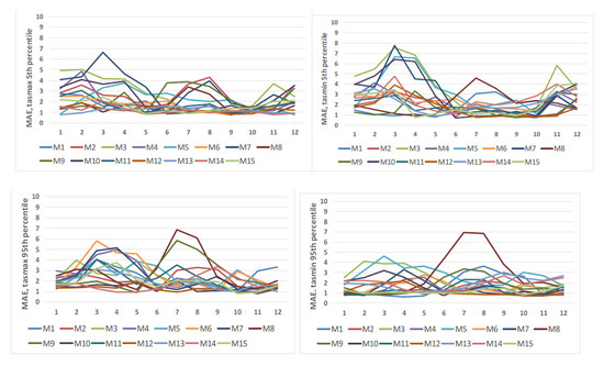
Figure 4.
Mean absolute error (MAE) for the 5th and 95th percentiles in case of daily tasmax and tasmin, EURO-CORDEX simulations (full names of individual models are given in Table 1) against ROCADA observation-derived datasets, over the period 1971–2000.
The spatial correlation was determined between modeled and observation-derived gridded values. Figure 5 presents the correlation coefficients over the 12 months for tasmin (left) and tasmax (right). A strong correlation was detected for annual mean values for both parameters (Table 2), but during the summer, three models revealed a weak correlation in tasmin (M9, M2, and M7).
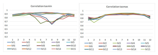
Figure 5.
Pearson correlation for tasmin (left) and tasmax (right) between EURO-CORDEX simulations (full names of individual models are given in Table 1) and ROCADA observation-derived datasets over the period 1971–2000.
In general, all the 15 RCMs can represent these variables within a reasonable range of uncertainty (Table S1). For tasmax, the MAE is between 0.7–5.3 °C having a median of 1.6 °C. More significant errors (higher than 4 °C) are present in March–April and July–August.
Regarding tasmin, the range of MAE is 0.6–5.4 °C with a median value of 1.5 °C. Larger errors (more than 4 °C) are present in February–April and July–August. The most extensive spread of errors was found for precipitation, where the MAE range of monthly precipitation is 6.2–59.4 mm with a median of 19.6 mm. Higher errors (more than 40 mm) were detected for May–August. The spatial representation of the variables was checked by a spatial correlation between model outputs and observations. The maximum temperature is represented very well. The median of the correlation coefficient throughout the year is 0.89, and the weakest correlation is 0.68 in February. In minimum temperature, the median value is 0.90, while the lowest correlation is 0.63 in August.
Even though the multimodel MAE, RMSE, and Corr are similar over the year, a significant spread among the models was found. The multimodel MAE for tasmax and tasmin is between 1.25 and 2.42 °C. More significant errors were found in tasmin in wintertime (in particular in the case of RCA4). This fact could be linked to a bias over snow-covered areas, as presented in Vautard et al., 2020 [20], assessing data from the northern part of Europe. The incoherencies are much more evident in the cold season for temperature and in the warm period for precipitation.
A similar weak representation of minimum temperature during summertime (here Figure 5) was also found in a previous study [20]. In summer, model biases are substantially dependent on stable boundary layer parameterizations due to lighter winds inducing less mixing than in winter.
3.2. Model Performance on Precipitation
Precipitation represents a critical variable in agroclimatology. The representation of precipitation in climate models shows significant uncertainties.
The validation metrics for the 15 RCMs are given in Figure 6, and the detailed results are presented in the Supplementary Material, Table S1. The multimodel mean of MAE is 144.1 mm (Table 2). There is a wide spread among the models over the year (upper left graph in Figure 6). The largest monthly MAEs are detected in the case of M7 and M8. The difference between RMSE and MAE highlights outliers in errors, especially in the summertime, particularly for the M4, M15, and M6 simulations (upper left graph in Figure 6). The monthly 95th percentiles were compared between modeled values and observation-derived data (lower left chart in Figure 6). Among the models, M8 seems to be an outlier.
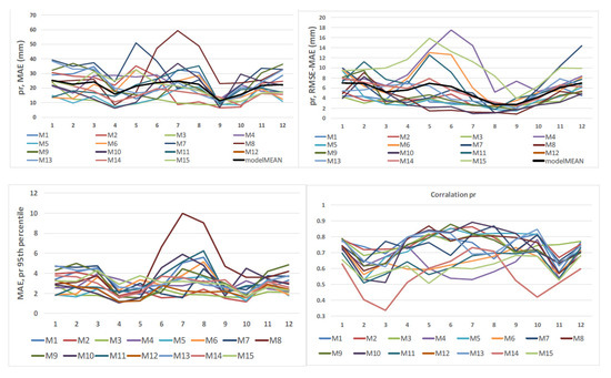
Figure 6.
Validation metrics for precipitation, EURO-CORDEX simulations (full names of individual models are given in Table 1) against ROCADA observation-derived data, over the period 1971–2000.
The weaker spatial correlations between models and observation-derived data (lower right graph in Figure 6) are also explained by regional climate models’ weakness in representing precipitation, mainly during the cold season.
In Figure 6, the differences between models and observations are calculated for monthly sums (larger values). In general, RCMs tend to overestimate precipitation, but more in winter than in summer (here Figure 6) [20]. In summer, rain is essentially absent in observations (especially in gridded ones, such as ROCADA), while most simulations produce rain through predominantly (parameterized) convective events. Regarding the importance of boundary conditions, both large-scale drivers and local physical parameterizations (e.g., convection, microphysics) are important in determining the biases [20].
A weaker spatial representation was found for precipitation, with a median value of 0.71, and the lowest correlation detected was 0.34 in March. For precipitation, Vautard et al., 2020 [20] found smaller biases in summer than in winter in Europe. We found a similar result for the multimodel MAE for the same seasons. Still, the presence of outliers in summer (in particular for the RCA4 regional model) is canceled out by averaging.
Regarding vegetation periods of maize (April–October) and winter wheat (October–June), the performance of the models is presented in Figure 7. The Taylor diagrams indicated a better fit for the winter wheat vegetation period with lower RMSE and stronger spatial correlation (see Table 2).
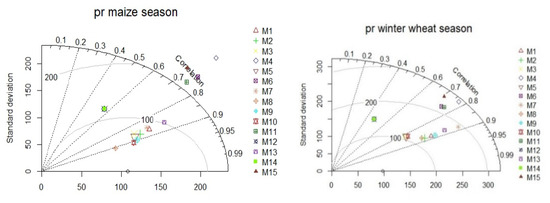
Figure 7.
Validation of pr in 15 EURO-CORDEX simulations against ROCADA observation-derived data, over the period 1971–2000 (full names of individual models are given in Table 1) for vegetation periods of maize (April–October) and winter wheat (October–June). In the diagram, the circle on Ox-axis represents the observation, and the colored plots represent the different models. Three statistics determine the relative places of the models: the Pearson correlation coefficient (curved axes), the centered RMS error (grey contours), and the standard deviation (Oy-axis). The model best fitting with observations will lie the nearest to the Ox-axis.
3.3. Model Selection Procedure
As shown in Section 3.1 and Section 3.2, there is a large spread among different RCMs in representing tasmax, tasmin, and pr. In this study, we applied a selection procedure for individual models to rank them, taking into account their performance in the case of each variable (Section 2.2.2).
At an annual scale, the top 5 models in terms of their performance are M9 (MOHC-HadGEM2-ES-IPSL-WRF381P_v1), M1 (CNRM-CM5-CLMcom-CCLM4-8-17_v1), M2 (CNRM-CM5-IPSL-WRF381P_v2), M10 (MOHC-HadGEM2-ES-KNMI-RACMO22E_v2), and M12 (MPI-M-MPI-ESM-LR-KNMI-RACMO22E_v1). Analysis by month revealed that M12 is the model that best fits in September, October, November, and December and is in the second position in July and August. For the other models, we have a much more diverse ranking over the months. M1 is placed in the top three positions (among all models) in the winter and spring months and is relatively low-ranked (below ninth place) in July, August, September, October. M10 indicated a reverse situation, ranking in the top three positions within the first three places during summer and autumn (June, July, August, and September). Still, it was assigned ranks below ninth position for the winter period (December, January, February, and March). For M2, the highest ranking was detected for February, June, October, and November, and the lowest in April, May, and December. The most significant difference in ranking during the year was found in M9, which performed best in February and March, but in July and December had a very weak performance.
Consequently, one can state that there are models with high performance in a given period of the year but with lower skills in the other months. These results are extremely important for the agriculture sector to select the models with the best performance during the vegetation periods for specific crops. They should be considered in agroclimatology studies and make the model selection accordingly to reduce the inconsistency among the model data. Similar to the monthly and annual mean values, a model ranking was calculated for the vegetation periods of maize (April–October) and of winter wheat (October–June) (Table 3). In the case of the vegetation period for maize crops, models with the highest rank are M12 (MPI-M-MPI-ESM-LR-KNMI-RACMO22E_v1), M2 (CNRM-CM5-IPSL-WRF381P_v2), M15 (MPI-M-MPI-ESM-LR-SMHI-RCA4_v1a), M9 (MOHC-HadGEM2-ES-IPSL-WRF381P_v1), and M10 (MOHC-HadGEM2-ES-KNMI-RACMO22E_v2). For the winter wheat crop, the best-fitting models are M1 (CNRM-CM5-CLMcom-CCLM4-8-17_v1), M9 (MOHC-HadGEM2-ES-IPSL-WRF381P_v1), M10 (MOHC-HadGEM2-ES-KNMI-RACMO22E_v2), M8 (MOHC-HadGEM2-ES-CLMcom-CCLM4-8-17_v1), and M12 (MPI-M-MPI-ESM-LR-KNMI-RACMO22E_v1) (Table 3).

Table 3.
Regional climate model ranking for months, for annual, and for vegetation periods of maize (April–October) and winter wheat (October–June) (full names of individual models are given in Table 1).
4. Conclusions and Discussion
In the study, 15 EURO-CORDEX simulations of tasmax, tasmin, and pr were validated against ROCADA observation-derived datasets for the Romanian arable land. The performance of the models was quantified by three validation metrics: MAE, RMSE, and spatial correlation. Consequently, we obtained different representations of maximum and minimum temperature as well as precipitation. For the vegetation periods of the two crops, a better fit for the maize vegetation period was revealed for temperature and for winter wheat crop when precipitation is considered.
Besides the significant differences in model skills over different months, several outliers were detected, inducing considerable errors in the multimodel means. Outliers are very model-dependent; they are the result of the model physics and setup, or they could be inherited from the driving GCMs. Thus, each case should be analyzed separately, but this is not the aim of this paper. For example, we found MOHC-HadGEM2-ES CLMcom-CCLM4-8-17_v1 as an outlier for tasmax and tasmin in high extremes (95th percentiles) and precipitation. References [15,20] also reported the unusual behavior of CCLM. In the case of CCLM, the spatial setup of the model (domain size and vertical resolution) has a more significant impact on performance than changes in the physical parameterization [30].
The larger ensemble spread for the lower quantiles of winter temperature (here Figure 4) can be due to the considerable sensitivity of winter temperatures on differences in the regional temperature field. Additionally, it may be due to the solid west–east air temperature gradient in winter in Europe and the snow-albedo feedback [31].
The presence of outliers could have a significant influence on random model selection. This is one of the main reasons why using a single model output for impact studies is not recommended. Furthermore, to capture the climate system’s main feature (dominant trend), the multimodel means are still not the perfect method because outliers also determine multimodel means. More realistic would be to use the entire ensemble climate sensitivity range to account for uncertainties in future climate. This type of interpretation, however, is quite difficult in impact modeling.
For this reason, the study recommends reducing the number of ensembles keeping the main climate features. Based on the validation metrics, a model ranking procedure was applied to quantify the overall skill of the individual models, including temperature and precipitation. The ranking procedure was elaborated for monthly and yearly means, as well as for vegetation periods.
In many cases, the model’s performance varies in the different periods of the year (e.g., seasons), and for this reason, the annual ranking is not recommended for the vegetation periods. Each vegetation period should be analyzed separately because the seasonal errors could lead to different rankings. In our case, the MOHC-HadGEM2-ES-IPSL-WRF381P_v1 simulation has the best performance at annual means. For the maize vegetation period, MPI-M-MPI-ESM-LR-KNMI-RACMO22E_v1 is the best model; for the wheat vegetation period CNRM-CM5-CLMcom-CCLM4-8-17_v1 is the best one. The best five models for the winter wheat crop are M1 (CNRM-CM5-CLMcom-CCLM4-8-17_v1), M9 (MOHC-HadGEM2-ES-IPSL-WRF381P_v1), M10 (MOHC-HadGEM2-ES-KNMI-RACMO22E_v2), M8 (MOHC-HadGEM2-ES-CLMcom-CCLM4-8-17_v1), and M12 (MPI-M-MPI-ESM-LR-KNMI-RACMO22E_v1). For the maize crop, the models with the highest five in the final ranking are M12 (MPI-M-MPI-ESM-LR-KNMI-RACMO22E_v1), M2 (CNRM-CM5-IPSL-WRF381P_v2), M15 (MPI-M-MPI-ESM-LR-SMHI-RCA4_v1a), M9 (MOHC-HadGEM2-ES-IPSL-WRF381P_v1), and M10 (MOHC-HadGEM2-ES-KNMI-RACMO22E_v2).
Regarding the structure of RCM and its driving model, there is no clear relationship between model type and performance. For example, the annual best rank was found for the MOHC-HadGEM2-ES-IPSL-WRF381P_v1 simulation, whereas the lowest position is also assigned to the IPSL-WRF381P_v1 RCM simulation but driven by the IPSL-CM5A-MR GCM. On the other hand, CLMcom-CCLM4-8-17_v1 driven by the same GCMs as the first one (MOHC-HadGEM2-ES) is situated in only eighth place.
Each RCM has its structure, and the performance depends on how its physics can capture large-scale and small-scale processes. Consequently, we obtained different representations of tasmax, tasmin, and pr. The models’ performance differs among variables and periods of the year. For this reason, we propose a ranking method taking into account the model performance for 18 metrics, also assessing the extremes. An example was given for five ensembles (having the lowest errors and highest correlations with observations) separately for maize and winter wheat vegetation seasons. The results are also presented on a monthly scale to combine the models for their particular use.
The results of this paper can be helpful for stakeholders for two main reasons: on the one hand, the number of the models can be significantly reduced, keeping only the models with the lowest errors, and on the other hand, the incoherencies among the models decrease by eliminating the outliers. These two aspects are very convenient for agronomical applications, where the climate is a crucial driving factor in a specific period of the year. It should be mentioned that bias-correction of raw model data is required in some applications, but this is beyond the scope of this article.
Supplementary Materials
The following are available online at https://www.mdpi.com/article/10.3390/atmos12080978/s1, Table S1: MAE and RMSE for monthly maximum temperature, minimum temperature and precipitation amount, 15 EURO-CORDEX simulations against ROCADA observations, 1971–2000; Table S2: Ranking scores for 15 EURO-CORDEX simulations for months, annual mean and means of vegetation periods of maize (April–October) and winter wheat (October–June), 1—the highest rank, 0—the lowest rank, Table S3: Weighted ranks for 15 EURO-CORDEX simulations for annual mean and means of vegetation periods of maize (April–October) and winter wheat (October–June).
Author Contributions
Conceptualization, A.-E.C. and B.B.; methodology, B.B., V.S. and A.-E.C.; software, A.-S.T. and C.S.; validation, A.-S.T., C.S. and B.B.; formal analysis, A.-E.C.; investigation, B.B. and A.-E.C.; resources, B.B., C.H., A.-E.C.; data curation, A.-S.T. and C.H.; writing—original draft preparation, B.B., A.-E.C., C.S.; writing—review and editing, B.B., A.-E.C., V.S.; visualization, C.H. and B.B.; supervision, B.B. and A.-E.C.; project administration, B.B.; funding acquisition, A.-E.C. and C.S. All authors have read and agreed to the published version of the manuscript.
Funding
This work was supported by a grant of the Romanian Ministry of Education and Research, CCCDI-UEFISCDI, project number PN-III-P2-2.1-PED-2019-2310, within PNCDI III.
Institutional Review Board Statement
Not applicable.
Informed Consent Statement
Not applicable.
Data Availability Statement
Not applicable.
Acknowledgments
This research was developed under the framework of the demonstration experimental project Redefining the agro-suitability zones for maize and winter wheat crops towards a smart climate change-oriented agriculture in Romania (www.agroclim.ro, accessed on 1 July 2021). The authors acknowledge the land use data freely provided by the Agency for Payment and Interventions in Agriculture in Romania (http://www.apia.org.ro/, accessed on 1 July 2021). We also acknowledge graphic technical support to Mugurel Raul Sidau.
Conflicts of Interest
The authors declare no conflict of interest.
References
- Field, C.; Barros, V.; Stocker, T.; Dahe, Q. IPCC—Managing the Risks of Extreme Events and Disasters to Advance Climate Change Adaptation: Special Report of the Intergovernmental Panel on Climate Change; Cambridge University Press: Cambridge, UK, 2012. [Google Scholar] [CrossRef]
- EU. EU Adaptation Strategy. 2019. Available online: https://ec.europa.eu/clima/policies/adaptation/what_en (accessed on 16 May 2021).
- EU. The Post-2020 Common Agricultural Policy: Environmental Benefits and Simplification. 2019. Available online: https://ec.europa.eu/info/sites/info/files/food-farming-fisheries/key_policies/documents/cap-post-2020-environ-benefits-simplification_en.pdf (accessed on 1 July 2021).
- EPA. Agrophenology. 2019. Available online: https://www.eea.europa.eu/data-and-maps/indicators/timing-of-the-cycle-of-2/assessment (accessed on 1 July 2021).
- Rummukainen, M. State-of-the-art with regional climate models. WIREs Clim. Chang. 2010, 1, 82–96. [Google Scholar] [CrossRef]
- Coppola, E.; Nogherotto, R.; Ciarlo, J.M.; Giorgi, F.; van Meijgaard, E.; Kadygrov, N.; Iles, C.; Corre, L.; Sandstad, M.; Somot, S.; et al. Assessment of the European Climate Projections as Simulated by the Large EURO-CORDEX Regional and Global Climate Model Ensemble. J. Geophys. Res. Atmos. 2021, 126. [Google Scholar] [CrossRef]
- Fischer, G.; Shah, M.; Tubiello, F.; van Velhuizen, H. Socio-economic and climate change impacts on agriculture: An integrated assessment, 1990–2080. Philos. Trans. R. Soc. Biol. Sci. 2005, 360, 2067–2083. [Google Scholar] [CrossRef]
- Lane, A.; Jarvis, A. Changes in Climate will modify the Geography of Crop Suitability: Agricultural Biodiversity can help with Adaptation. SAT Ejournal 2007, 4, 1–12. [Google Scholar]
- Ovalle-Rivera, O.; Läderach, P.; Bunn, C.; Obersteiner, M.; Schroth, G. Projected shifts in Coffea arabica suitability among major global producing regions due to climate change. PLoS ONE 2015, 10, e0124155. [Google Scholar] [CrossRef] [PubMed] [Green Version]
- Ranjitkar, S.; Sujakhu, N.M.; Merz, J.; Kindt, R.; Xu, J.; Matin, A.; Zomer, R.J. Suitability analysis and projected climate change impact on banana and coffee production zones in Nepal. PLoS ONE 2016, 11, e0163916. [Google Scholar] [CrossRef] [PubMed] [Green Version]
- De Silva, C.S.; Weatherhead, E.K.; Knox, J.W.; Rodriguez-Diaz, J.A. Predicting the impacts of climate change-A case study of paddy irrigation water requirements in Sri Lanka, Agric. Water Manag. 2007, 93, 19–29. [Google Scholar] [CrossRef]
- Liu, J.; Fritz, S.; Van Wesenbeeck, C.F.A.; Fuchs, M.; You, L.; Obersteiner, M.; Yang, H. A spatially explicit assessment of current and future hotspots of hunger in Sub-Saharan Africa in the context of global change. Glob. Planet. Chang. 2008, 64, 222–235. [Google Scholar] [CrossRef]
- Teixeira, E.I.; Fischer, G.; Van Velthuizen, H.; Walter, C.; Ewert, F. Global hot-spots of heat stress on agricultural crops due to climate change. Agric. For. Meteorol. 2013, 170, 206–215. [Google Scholar] [CrossRef]
- Zabel, F.; Putzenlechner, B.; Mauser, W. Global Agricultural Land Resources—A High Resolution Suitability Evaluation and Its Perspectives until 2100 under Climate Change Conditions. PLoS ONE 2014, 9, e114980. [Google Scholar] [CrossRef] [PubMed] [Green Version]
- Kotlarski, S.; Keuler, K.; Christensen, O.B.; Colette, A.; Déqué, M.; Gobiet, A.; Goergen, K.; Jacob, D.; Lüthi, D.; van Meijgaard, E. Regional climate modeling on European scales: A joint standard evaluation of the EURO-CORDEX RCM ensemble. Geosci. Model Dev. 2014, 7, 1297–1333. [Google Scholar] [CrossRef] [Green Version]
- Forestieri, A.; Arnone, E.; Blenkinsop, S.; Candela, A.; Fowler, H.; Noto, L.V. The impact of climate change on extreme precipitation in Sicily, Italy. Hydrol. Process. 2018, 32, 332–348. [Google Scholar] [CrossRef] [Green Version]
- Torma, C.Z. Detailed validation of EURO-CORDEX and Med-CORDEX regional climate model ensembles over the Carpathian Region. Időjárás 2019, 123, 217–240. [Google Scholar] [CrossRef]
- Warscher, M.; Wagner, S.; Marke, T.; Laux, P.; Smiatek, G.; Strasser, U.; Kunstmann, H. A 5 km Resolution Regional Climate Simulation for Central Europe: Performance in High Mountain Areas and Seasonal, Regional and Elevation-Dependent Variations. Atmosphere 2019, 10, 682. [Google Scholar] [CrossRef] [Green Version]
- Varga, Á.J.; Breuer, H. Sensitivity of simulated temperature, precipitation, and global radiation to different WRF configurations over the Carpathian Basin for regional climate applications. Clim. Dyn. 2020, 55, 2849–2866. [Google Scholar] [CrossRef]
- Vautard, R.; Kadygrov, N.; Iles, C.; Boberg, F.; Buonomo, E.; Bülow, K.; Coppola, E.; Corre, L.; Meijgaard, E.; Nogherotto, R. Evaluation of the large EURO-CORDEX regional climate model ensemble. J. Geophys. Res. Atmos. 2020. [Google Scholar] [CrossRef]
- Ceglar, A.; Croitoru, A.-E.; Cuxart, J.; Djurdjevic, V.; Güttler, I.; Ivančan-Picek, B.; Jug, D.; Lakatos, M.; Weidinger, T. PannEx: The Pannonian Basin Experiment. Clim. Serv. 2018, 11, 78–85. [Google Scholar] [CrossRef]
- Dumitrescu, A.; Birsan, M.V. ROCADA: A gridded daily climatic dataset over Romania (1961–2013) for nine meteorological variables. Nat Hazards 2015, 78, 1045–1063. [Google Scholar] [CrossRef]
- Klein Tank, A. Changing temperature and precipitation extremes in Europe’s climate. Change 2002, 63, 14–16. [Google Scholar]
- Website of the European Climate Assessment & Dataset project. Available online: https://www.ecad.eu/ (accessed on 16 May 2021).
- Website of CARPATCLIM Project. Available online: http://www.carpatclim-eu.org (accessed on 16 May 2021).
- Sidău, M.R.; Croitoru, A.-E.; Alexandru, D.-E. Comparative Analysis between Daily Extreme Temperature and Precipitation Values Derived from Observations and Gridded Datasets in North-Western Romania. Atmosphere 2021, 12, 361. [Google Scholar] [CrossRef]
- Birsan, M.-V.; Dumitrescu, A. ROCADA: Romanian daily gridded climatic dataset (1961–2013) V1.0. Adm. Natl. Meteorol. Bucur. Rom. PANGAEA 2014. [Google Scholar] [CrossRef]
- Website of EURO-CORDEX—Coordinated Downscaling Experiment—European Domain. Available online: https://euro-cordex.net/index.php.en (accessed on 16 May 2021).
- Bartók, B.; Tobin, I.; Vautard, R.; Vrac, M.; Jin, X.; Levavasseur, G.; Denvil, S.; Dubus, L.; Parey, S.; Michelangeli, P.-A.; et al. Climate projection dataset tailored for the European energy sector. Clim. Serv. 2019, 16, 1001383. [Google Scholar] [CrossRef]
- Suklitsch, M.; Gobiet, A.; Leuprecht, A.; Frei, C. High Resolution Sensitivity Studies with the Regional Climate Model CCLM in the Alpine Region. Meteorol. Z. 2008, 17, 467–476. [Google Scholar] [CrossRef]
- Le Roy, B.; Lemonsu, A.; Schoetter, R. A statistical–dynamical downscaling methodology for the urban heat island applied to the EURO-CORDEX ensemble. Clim. Dyn. 2021, 56, 2487–2508. [Google Scholar] [CrossRef]
Publisher’s Note: MDPI stays neutral with regard to jurisdictional claims in published maps and institutional affiliations. |
© 2021 by the authors. Licensee MDPI, Basel, Switzerland. This article is an open access article distributed under the terms and conditions of the Creative Commons Attribution (CC BY) license (https://creativecommons.org/licenses/by/4.0/).