Implementation of a Lagrangian Stochastic Particle Trajectory Model (LaStTraM) to Simulate Concentration and Flux Footprints Using the Microclimate Model ENVI-Met

Abstract

The number of studies evaluating flux or concentration footprints has grown considerably in recent years. These footprints are vital to understand surface–atmosphere flux measurements, for example by eddy covariance. The newly developed backwards trajectory model LaStTraM (Lagrangian Stochastic Trajectory Model) is a post-processing tool, which uses simulation results of the holistic 3D microclimate model ENVI-met as input. The probability distribution of the particles is calculated using the Lagrangian Stochastic method. Combining LaStTraM with ENVI-met should allow us to simulate flux and concentration footprints in complex urban environments. Applications and evaluations were conducted through a comparison with the commonly used 2D models Kormann Meixner and Flux Footprint Predictions in two different meteorological cases (stable, unstable) and in three different detector heights. LaStTraM is capable of reproducing the results of the commonly used 2D models with high accuracy. In addition to the comparison with common footprint models, studies with a simple heterogeneous and a realistic, more complex model domain are presented. All examples show plausible results, thus demonstrating LaStTraM’s potential for the reliable calculation of footprints in homogeneous and heterogenous areas.

1. Introduction

The number of study sites for the measurement of the surface–atmosphere exchange of energy and matter such as greenhouse gases (i.e., carbon dioxide, methane, nitrous oxide) has grown substantially during recent years [1,2,3]. Flux data are used to increase process understanding of the terrestrial carbon cycle, to constrain models, and to inform policy makers, e.g., in the context of climate change research and for modeling purposes. The state-of-the-art method which is used at measurement sites is the eddy covariance technique. For an accurate interpretation of the flux data, it is necessary to estimate the surface area that influences the signal measured at the detector location, which is the so-called flux footprint or flux source area [4,5,6]. The concentration or flux footprint of a quantity is a function of the characteristics of the Earth’s surface, the state of the atmosphere as well as the height of the detector above ground level. At the surface, the distribution of sources and sinks (homogenous/heterogeneous), the surface roughness length, and the topography are important factors in shaping the footprint’s location and dimensions. Atmospheric stability, wind speed and direction, as well as turbulent intensity are atmospheric factors influencing the footprint. For this purpose, several models have been published since the 1990s which can be distinguished into four categories: (1) analytical models [7,8,9,10,11,12]; (2) Lagrangian stochastic particle dispersion models (LS) [13,14]; (3) large-eddy simulations (LES) [15,16,17]; and (4) closure models [18,19,20].

Most of the available footprint models are valid only in case of a homogeneous source and in flat topography. This includes all models based on analytically derived mathematical expressions to calculate advection and diffusion of the quantity of interest. LES footprint models [16] and closure models [20] overcome this limitation, i.e., they are able to simulate fluxes in heterogeneous environments, e.g., high vegetation, forests, and urban areas. One characteristic of the first mentioned type of models is the high computational demand. This means that only computer clusters with hundreds of processors are able to calculate footprints in reasonable time. In contrast, Reynolds-Averaged Navier–Stokes (RANS) models have lower computational demand and can hence run on personal computers. However, as Hellsten et al. [16] state there is no backward-integration approach for any building-resolving LES-LS footprint predictions available yet. Backward-integration approaches represent a backward tracking of particles from the target (detector) to the source (emission source). Compared to forward tracking from source to target, where a multitude of particles is tracked without ever reaching the detector zone, backward approaches feature a significantly higher computational efficiency as the number of particles eventually reaching the detector zone is already determined at simulation start. That allows us to define smaller detector zones to be thus comparable with real measurement devices [14].

In the present study, the microclimate model ENVI-met [21], a RANS model, was coupled to a newly developed Lagrangian model called LaStTraM (Lagrangian Stochastic Trajectory Model) to simulate particle trajectories with a backward-integration approach based on the microclimate’s three-dimensional output data in order to close this gap. Since ENVI-met features a sophisticated plant physiology stomata model (A-gs; [22]) to simulate transpiration and carbon uptake of plants, the influences of heterogeneous sources and source distributions (e.g., trees, shrubs, grass) on the footprint can be modelled in complex topographies (e.g., within dense and complex urban areas) [23,24]. LaStTraM works with all ENVI-met versions including the free LITE version.

To evaluate the capability of the newly developed post-processing Lagrangian model to simulate footprints in a homogeneous scenario, the model results are compared to a well-known Lagrangian model from Kljun et al. [9,10] and an analytic model from Kormann and Meixner [11]. Furthermore, the influence of heterogeneous sources in more complex model areas on the concentration and the flux footprint is discussed.

2. Model Description

In an offline coupling, all necessary atmospheric parameters for the calculations of LaStTraM are taken from simulation outputs provided by the microclimate model ENVI-met. The model ENVI-met is a prognostic, three-dimensional, high resolution microclimate model. With its physical fundamentals that are based on the principles of fluid mechanics, thermodynamics, and the laws of atmospheric physics, it is able to calculate three-dimensional wind fields, turbulence, air temperature and humidity, radiative fluxes, and building physics [25,26].

One of the key features of ENVI-met is the detailed modeling of vegetation. With its high spatial resolution (<5 m), ENVI-met allows the simulation of the individual photosynthesis rates, taking into account local solar radiation, air temperature and humidity, wind speed, and CO₂ concentration, among other parameters [23].

The spatial and temporal evolution of the wind field is calculated by applying the non-hydrostatic three-dimensional Navier–Stokes equation. Using the Boussinesq approximation, the density of air can be assumed to be constant [21,25,27]. Turbulence in ENVI-met is parametrized using a $E-\epsilon$ 1.5 order closure model. The $E-\epsilon$ model basically consists of two prognostic equations, one describing the production of turbulent kinetic energy (TKE) and the other its dissipation. In contrast to first order closure models, the $E-\epsilon$ model allows the simulation of advective processes in horizontally inhomogeneous environments without as much computation time as closure models of higher order [25,28].

The trajectory model horizontally and temporally interpolates all atmospheric parameter outputs from ENVI-met, making it quasi-independent of the ENVI-met model resolution. Both the interpolation as well as the advection of the particles are computed in parallel, making use of all available processor cores. The particles are released simultaneously at the start of a simulation. The interval in which simulation outputs are generated can be set by the user.

To simulate particle trajectories, LaStTraM operates with a backward-integration approach. The particles are “emitted” from the detector and are followed until predefined conditions are met, e.g., particles reach coordinates where plants or sources of different compounds, such as CO₂, are located. The particles’ starting position can either be set to the center of the detector or can be randomly generated inside the detector’s dimensions. The number of particles to be simulated can be freely set by the user. All particles reaching certain areas are individually saved with various pieces of information such as their current three-dimensional position as well as their take off and touch down velocities.

2.1. Dynamic Interpolation of the 3D Model Domain

To reduce the dependencies of the simulation on the ENVI-met model resolution, all ENVI-met model output variables are dynamically interpolated for every particle and every timestep. The interpolation is carried out using inverse distance weighting (IDW) of all adjacent atmospheric ENVI-met grids to the particle in a 3D Moore neighborhood analysis, i.e., a maximum of 27 neighboring grids are taken into the interpolation [29]:

$${\widehat{R}}_{int}={\displaystyle \sum }_{P_{i-1,j,k}}^{P_{i+1,j,k}}{\displaystyle \sum }_{P_{i,j-1,k}}^{P_{i,j+1,k}}{\displaystyle \sum }_{P_{i,j,k-1}}^{P_{i,j,k+1}}w\left(i,j,k\right)·R\left(i,j,k\right)$$

(1)

where $i,j,k$ are the ENVI-met grid coordinates of the particle, ${\widehat{R}}_{int}$ as the interpolated value, $R\left(i,j,k\right)$ are the ENVI-met model value of the in the grid $i,j,k$ and $w\left(i,j,k\right)$ are the weight corresponding to the grid cell $i,j,k$ calculated by:

$$w\left(i,j,k\right)=\frac{d{\left(i,j,k\right)}^{-1}}{{{\displaystyle \sum }}_{P_{i-1,j,k}}^{P_{i+1,j,k} }{{\displaystyle \sum }}_{P_{i,j-1,k}}^{P_{i,j+1,k}}{{\displaystyle \sum }}_{P_{i,j,k-1}}^{P_{i,j,k+1}}d{\left(i,j,k\right)}^{-1}}$$

(2)

where $d(i,j,k$) are the Euclidean distance calculated using the 3D Pythagorean Theorem between the particles’ actual position and the center of all adjacent atmospheric ENVI-met grid cells. Summing up all individual weights, the result must be equal to 1.

In case the particles’ vertical position lies below the center of the lowest ENVI-met atmospheric grid cell, the interpolation of the wind vectors $u$, $v$, $w$ is carried out using a logarithmic approach:

$$\begin{gathered} u_{int}=u_{k_0} · \ln \left(\frac{P_z}{z_0}\right)\ln {\left(\frac{h_{k_0,c}}{z_0}\right)}^{-1} \\ {v}_{int}=v_{k_0} · \ln \left(\frac{P_z}{z_0}\right)\ln {\left(\frac{h_{k_0,c}}{z_0}\right)}^{-1} \\ w=w_{k_0} · \ln \left(\frac{P_z}{z_0}\right)\ln {\left(\frac{h_{k_0,c}}{z_0}\right)}^{-1} \end{gathered}$$

(3)

where $u_{k_0}$, $v_{k_0}$, $w_{k_0}$ are the wind speed at the lowest ENVI-met atmospheric grid cell, $z_0$ is the roughness length of the surface, and $h_{k_0,c}$ is the height of the center point of the lowest ENVI-met grid cell, k = 0.

2.2. The Lagrangian Stochastic Model

Based on Weil et al. 2004 [30], the particles advection is calculated by:

$$P_{pos\left(x,y,z\right),t+∆t}=P_{pos\left(x,y,z\right),t}+P_{V,t}·∆t$$

(4)

where $P_{pos\left(x,y,z\right),t+∆t}$ is the new position of the particle after the time interval, $∆t$, $P_{pos\left(x,y,z\right),t}$ is the original position of the particle, and $P_{V,t}$ is the velocity of the particle. The velocity consists of two parts: a resolved, deterministic part ($P_{v_{res}}$) that is directly simulated based on the interpolated 3D wind vector fields of ENVI-met and a stochastic, random part ($P_{V_{LS}}$):

$$P_V=P_{v_{res}}+P_{V_{LS}}$$

(5)

The resolved velocity part $P_{v_{res}}$ is calculated by interpolating the u, v, w wind vectors for every particle position (see Equation (3)). The stochastic term of Equation (5), $P_{V_{LS}}$, is derived from the work of Weil et al., 2004 [30], where the considerations of Thomson, 1987 [31] are adapted. With these considerations and in accordance to Maronga et al., 2015 [32] and Steinfeld et al., 2008 [33], the difference in the particle’s stochastic velocity is calculated by:

$$d{P}_{V_{LS}}=\frac{3f_s{C}_0\epsilon }{4}\frac{P_{V_{LS}}}{e_s}dt+\frac{1}{2}\left(e_s^{-1}\frac{d{e}_s}{dt}{P}_{V_{LS}}+\frac{2}{3}\nabla e_s\right)+{\left(f_s{C}_0\epsilon \right)}^{\frac{1}{2}}d\xi$$

(6)

where $C_0$ is a universal constant of the structure function (here set to 3; as in [14]), $\epsilon$ and $e_s$ as the inverse distance interpolated (see Equations (1) and (2)) dissipation and TKE, respectively, $d\xi$ as a random displacement vector whose components are independent from each other and in time [32,33,34]. The random number is calculated using a normal (Gaussian) distribution where the interval is limited to $\pm 5.0\sigma$. The parameter $f_s$ defines the subgrid-scale TKE fraction of the total TKE [30,33].

For the conditions at the boundary surfaces of buildings and digital elevation models (DEM), the simulation can be operated in two modes: an iterative solution mode, where in case a particle’s new position was located inside a surface (buildings, DEM) the advection (Equation (8)) would be calculated with new random terms (${(f_s{C}_0\epsilon )}^{\frac{1}{2}}d\xi$) until a new position outside a solid structure is found or the maximum of 300 attempts is reached. In case no solution is found, the particle’s position will be set to the previous time step. In the second mode, the termination mode, all particles that enter a solid surface (buildings, DEM) are no longer tracked and removed from the simulation. Regardless of the boundary surfaces mode the model operates with, the particles that would enter ground surface will be set to a minimum height of the user’s choice (default value 0.0001 m). All particles leaving the lateral or top boundary of the model domain are removed.

While the resolved, deterministic velocity part of particles could be calculated in quite large time steps depending on grid size and velocity (e.g., CFL-Condition), the calculation of particles’ Lagrangian stochastic velocity demand much smaller timescales [30].

$$d{t}_{LS}=\frac{4e_s}{3f_s{C}_0\epsilon }$$

(7)

To ensure small time steps, an upper limit of at least $d{t}_{LS}/40$ is defined [32].

3. Footprint Calculation

A range of information is stored for every particle that reaches its target. This information includes the starting position within the detector, the final position within an emitter, travelled distance, elapsed time, mean velocity, as well as initial and final wind vector velocity. Since all data are stored for every particle reaching its target, the resulting file might be quite large (e.g., ~5 GB for around 20,000,000 particles reaching a source area).

To determine the relative contribution of a source to a measured concentration or flux at a predefined detector area, calculations can be performed that determine which surfaces/objects in a model area contribute to a measured concentration and flux at a given volume in space using the data information of the particles. The calculations of the concentration footprint $C$ and the flux footprint $F$ are carried out in accordance to Vesala et al. [5] and Flesch [35]:

$$C\left(x,y,z\right)=\frac{2}{N}{\displaystyle \sum }_{i=1}^n\frac{1}{w_{Emit,i}}Q\left(x,y,z\right)$$

(8)

$$F\left(x,y,z\right)=\frac{2}{N}{\displaystyle \sum }_{i=1}^n\frac{w_{Det,i}}{w_{Emit,i}}Q\left(x,y,z\right)$$

(9)

where $x,y,z$ are the grid coordinates, $Q$ is the source’s strength, $N$ is the total number of particles, $n$ is the number of particles reaching the detector zone. ${\displaystyle \sum }_{i=1}^n$ represents the sum of all particles reaching the target zone, $w_{Det,i}$ the initial $w$ component at a particle’s release at starting point within the detector zone and $w_{Emit,i}$ is the $w$ component of wind velocity at touch down at source area [5,36].

3.1. Simulating Footprints in Homogeneous Model Area—Comparison with Other Models

In order to evaluate the newly developed model, it is compared against two established and well-known footprint models: the Flux Footprint Predictions model (FFP) by Kljun et al. [14] and the analytic Kormann–Meixner model (K–M; Kormann and Meixner [11]). To prove the functionality of the newly developed model LaSTraM, the presented evaluation is held similar to the analysis of these models. It is hence based on two common meteorological cases (stable and unstable) and features the same corresponding detector heights (3 m, 20 m, and 40 m).

The analyzed model area is similar to the one used in Kljun et al. [14]. It consists of 400 × 400 × 40 grids with a horizontal resolution of 5 m and a vertical resolution of 2 m in a non-equidistant gridding, where the lowest grid cell is split into five subcells. The total extent of the area is thus 2000 m × 2000 m × 70 m. The model area features no building structures or other obstacles, the soil was digitized as “loamy soil”, and the vegetation was set to grass of 0.2 m height throughout the whole model area, thus creating a homogeneous case.

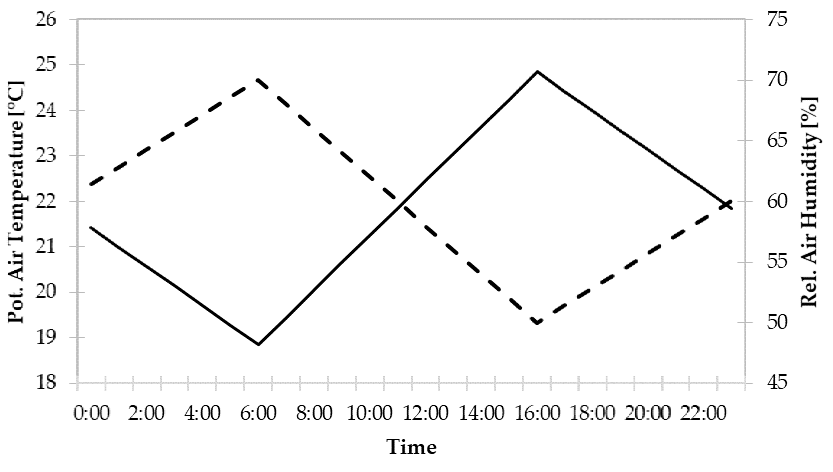
The ENVI-met simulation was set to start at 6 am on June 23rd, the simulation ran for 24 simulation hours. The meteorological boundary conditions can be seen in Figure 1, the boundary conditions for wind speed and direction were constant and set to 2 m s⁻¹ in 10 m height and 90° over the whole simulation time. The post-processing analysis in LaStTraM was run using the model outputs of the ENVI-met simulations. Each simulation featured 10⁸ particles. It took around 5.5 h to simulate the trajectories of the released 100 million particles in the 2 km × 2 km large area on a personal computer with an Intel Core i7-6700 CPU @ 3.40GHz (

Table 1. Simulated particles and simulation duration per examined scenario.

Time	Simulated Particles	Simulation Time
15:00 h (unstable case)	108	5 h 21 min
03:00 h (stable case)	108	5 h 46 min

).

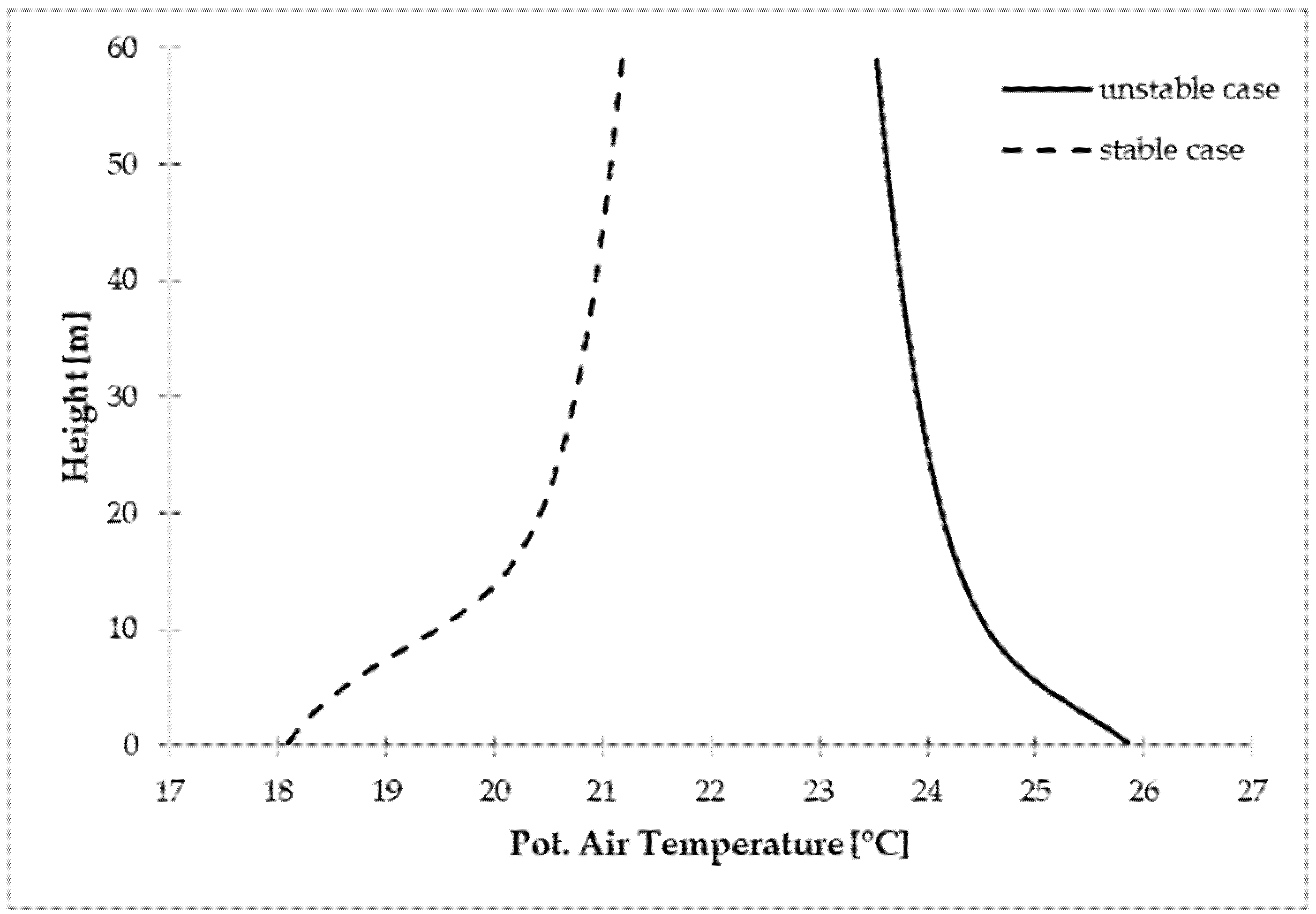
The footprint is sensitive to atmospheric stability, surface roughness, measurement height, and wind direction [5,14]. Since the atmospheric stability is a prognostic parameter of the microclimate model ENVI-met, the output files have to be analyzed to differentiate between unstable, stable, and neutral conditions. Analysis of the different output files showed an unstable atmosphere at 15:00 h and a stable atmosphere in the early morning hours around 3:00 h (see Figure 2). In order to compare the LaStTraM results with Kljun et al., 2002 [14] and Kormann and Meixner, 2001 [11], the output files of these hours have been used for the further analysis.

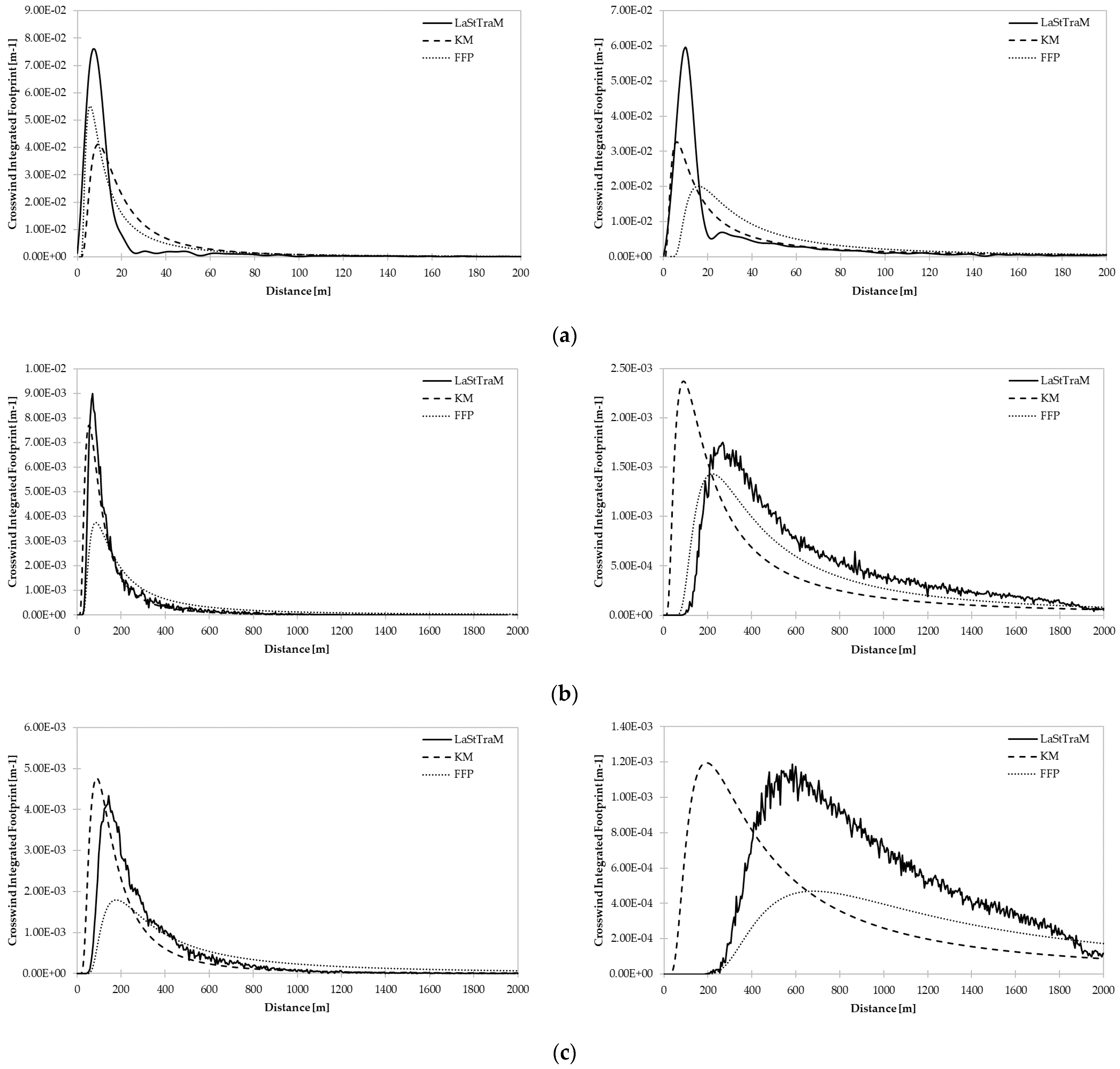
To compare the flux footprint results simulated with LaStTraM against the FFP model and the K–M-model, simulations using combinations of different detector heights (3 m, 20 m and 40 m) and atmospheric stabilities (15:00 h unstable case and 03:00 h stable case) were conducted.

Apart from the friction velocity ($u^{*}$), all input parameters for the FFP and K–M model could be directly extracted from the output data of ENVI-met. The friction velocity ($u^{*}$) was then calculated by:

$$u^{*}=\frac{u\times \kappa }{\ln \left(\frac{h}{z_0}\right)}$$

(10)

where $u$ is the wind speed, $\kappa$ the von Karman constant (here 0.4), $h$ is the height above ground, and $z_0$ as the roughness length.

Table 2. Input parameters for running the models FFP and K–M.

Parameter	Detector 3 m	Detector 20 m	Detector 40 m
Vegetation height (zveg)	0.2 m	0.2 m	0.2 m
Detector height (zsens40m)	3.25 m	20.5 m	40.5 m
Displacement height (d)	2/3 × zveg = 0.134 m
Measurement height above vegetation (z40m)	3.116 m	20.366 m	40.366 m
Mean wind speed at zm unstable (umeanday)	1.26 m/s	1.86 m/s	2.00 m/s
Mean wind speed at zm stable (umeannight)	1.26 m/s	1.86 m/s	2.02 m/s
Boundary layer height unstable (hday)	2500 m
Boundary layer height stable (hnight)	800 m
Obukhov length unstable (olday)	−7.55 m	−7.52 m	−7.51 m
Obukhov length stable (olnight)	18.99 m	19.22 m	19.25 m

shows all input parameters used to run FFP and K–M models.

3.2. Simulating Footprints in an Inhomogeneous Model Area

By coupling LaStTraM with ENVI-met’s three-dimensional model outputs, the model is able to simulate footprints in model areas featuring obstacles such as buildings or vegetation. To evaluate the influence of obstacles on the footprint, a simple inhomogeneous and one complex realistic scenario were analyzed.

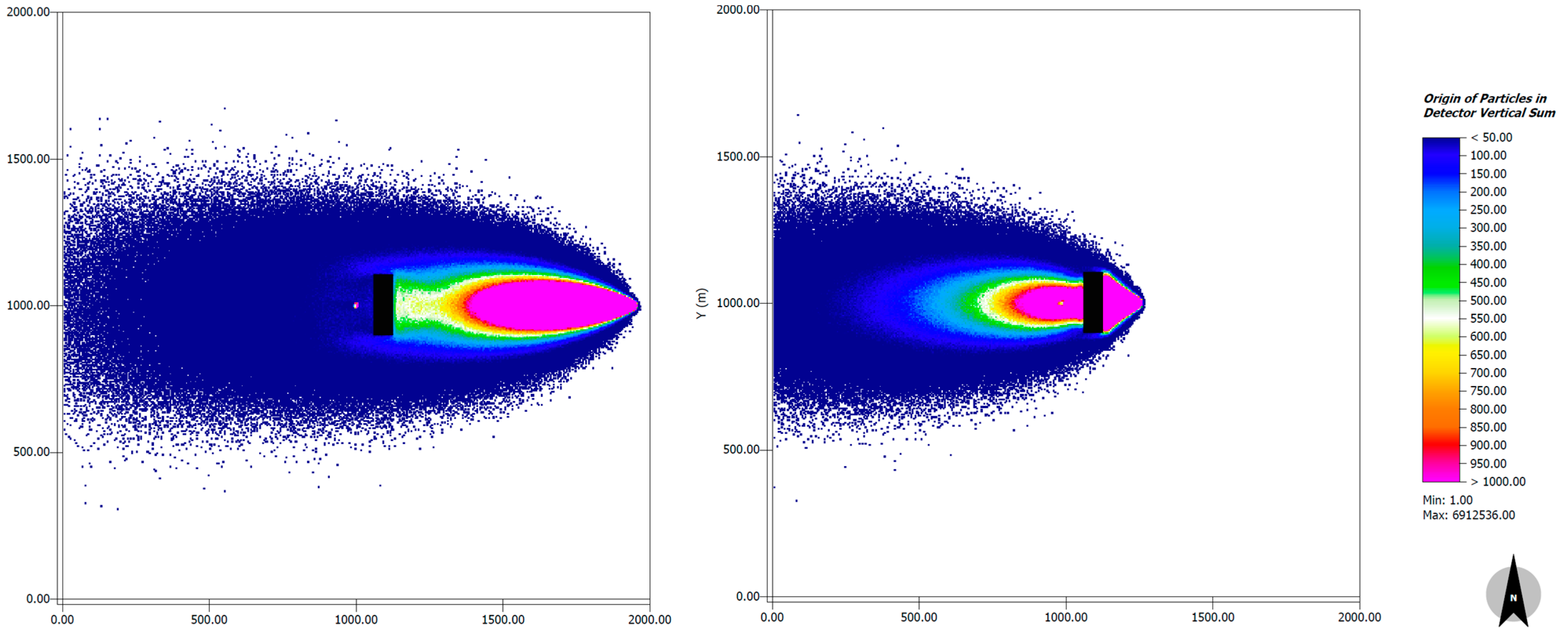
In the simple inhomogeneous scenario, a symmetrical obstacle (building) with a height of 20 m and a tree is added to the homogeneous model area. The detector is then placed in 3 m above ground at different distances to the obstacle (125 m and 820 m upwind distance from the obstacle) (see Figure 3).

The simple inhomogeneous model run featured identical meteorological boundary conditions as the homogeneous model run. To reduce the computational cost, the model was only run for the unstable case at 15:00 h.

3.3. Simulating Footprints in Realistic Model Area

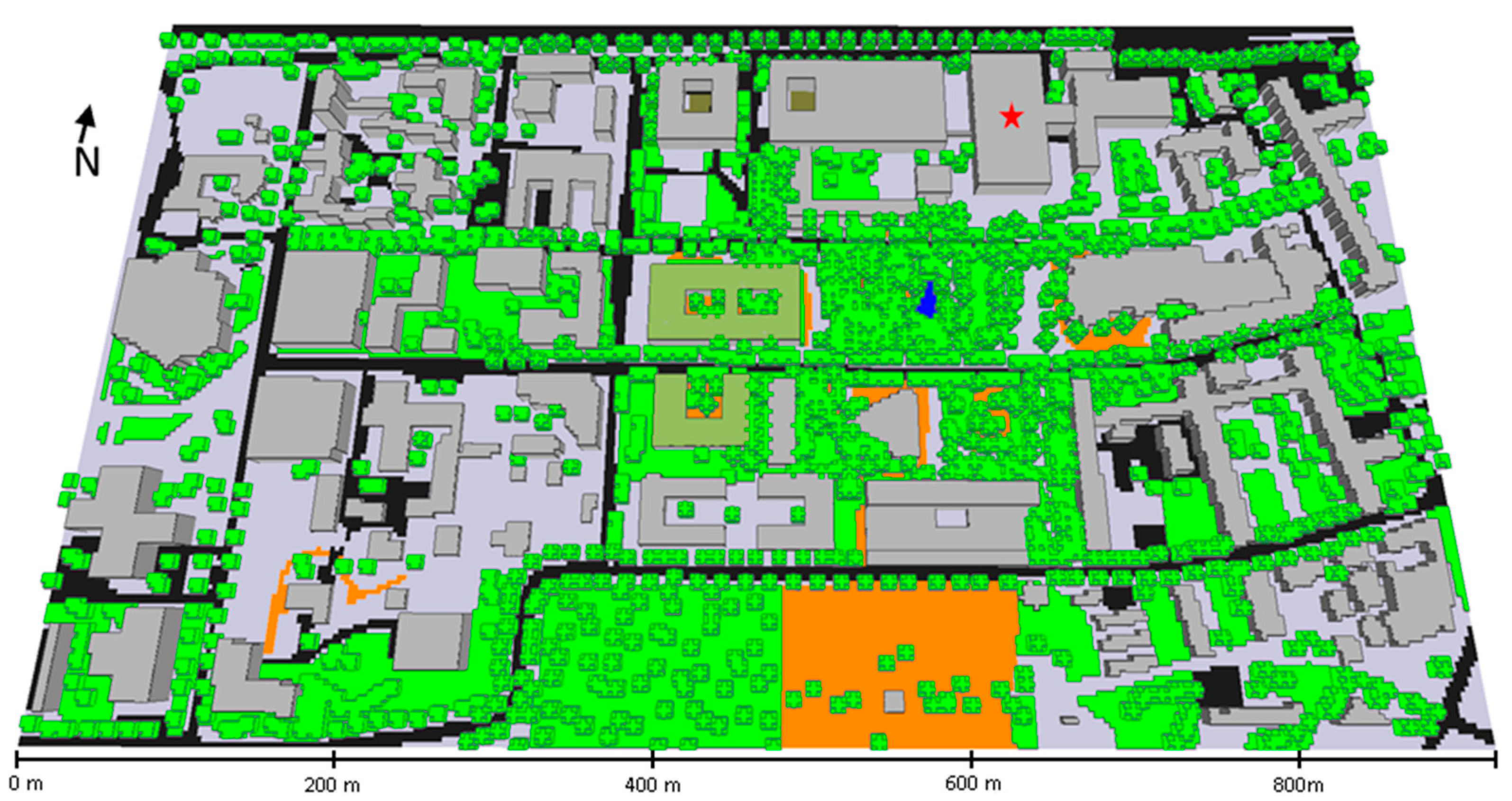
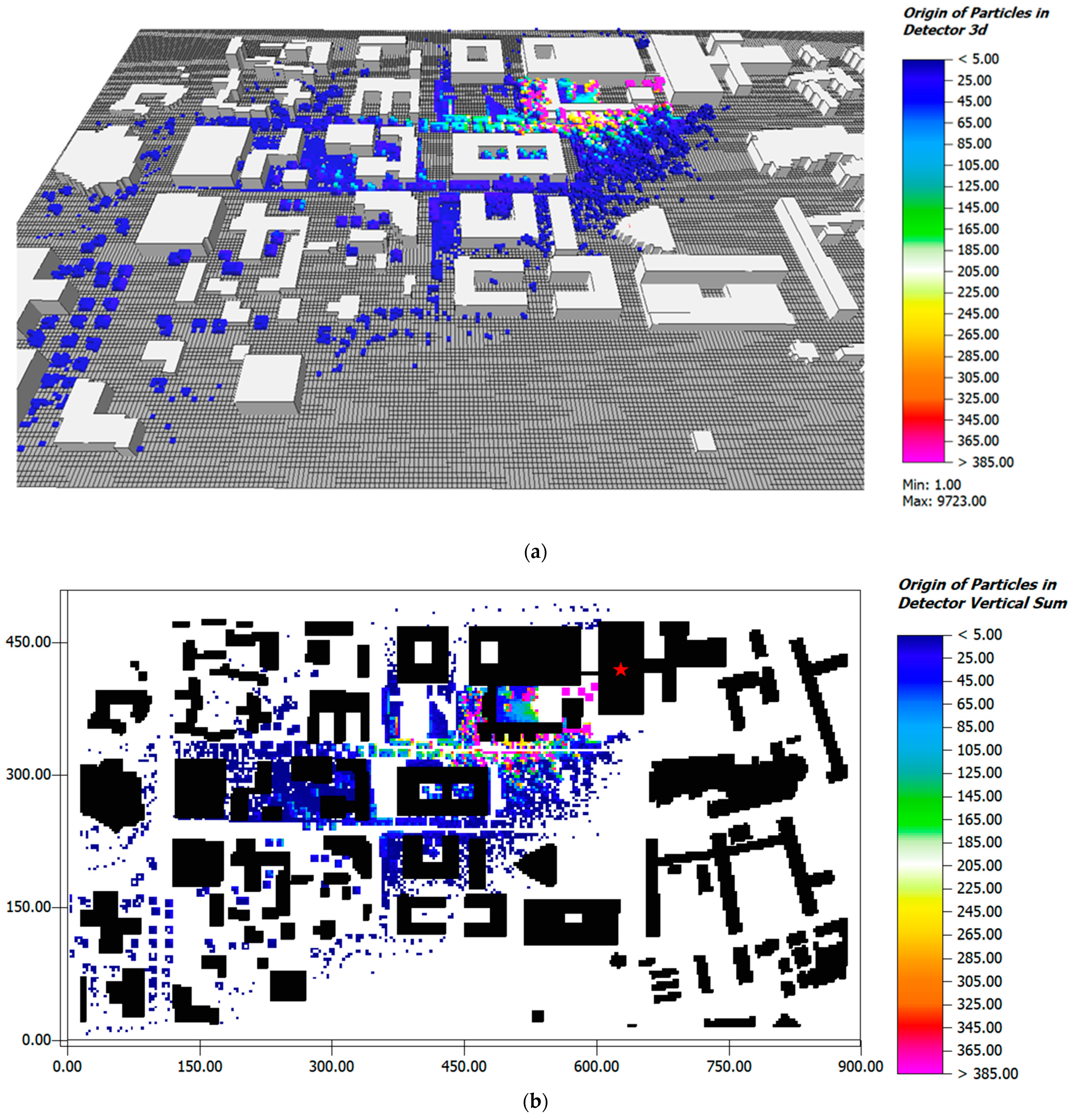
In a realistic scenario, the performance of LaStTraM is evaluated in an urban model area featuring buildings, different soil, and surface materials, as well as vegetation (see Figure 4). While this scenario, due to the lack of empirical data, cannot be seen as proving that the model is operating accurately in a complex environment, the scenario is designed to be a showcase visualizing the capabilities of the model.

The model area is located in Mainz, Germany and extends over 900 m × 510 m horizontally and 200 m vertically in a 3 m × 3 m × 2.5 m resolution. Again, a non-equidistant gridding, where the lowest grid cell is split into five subcells is chosen.

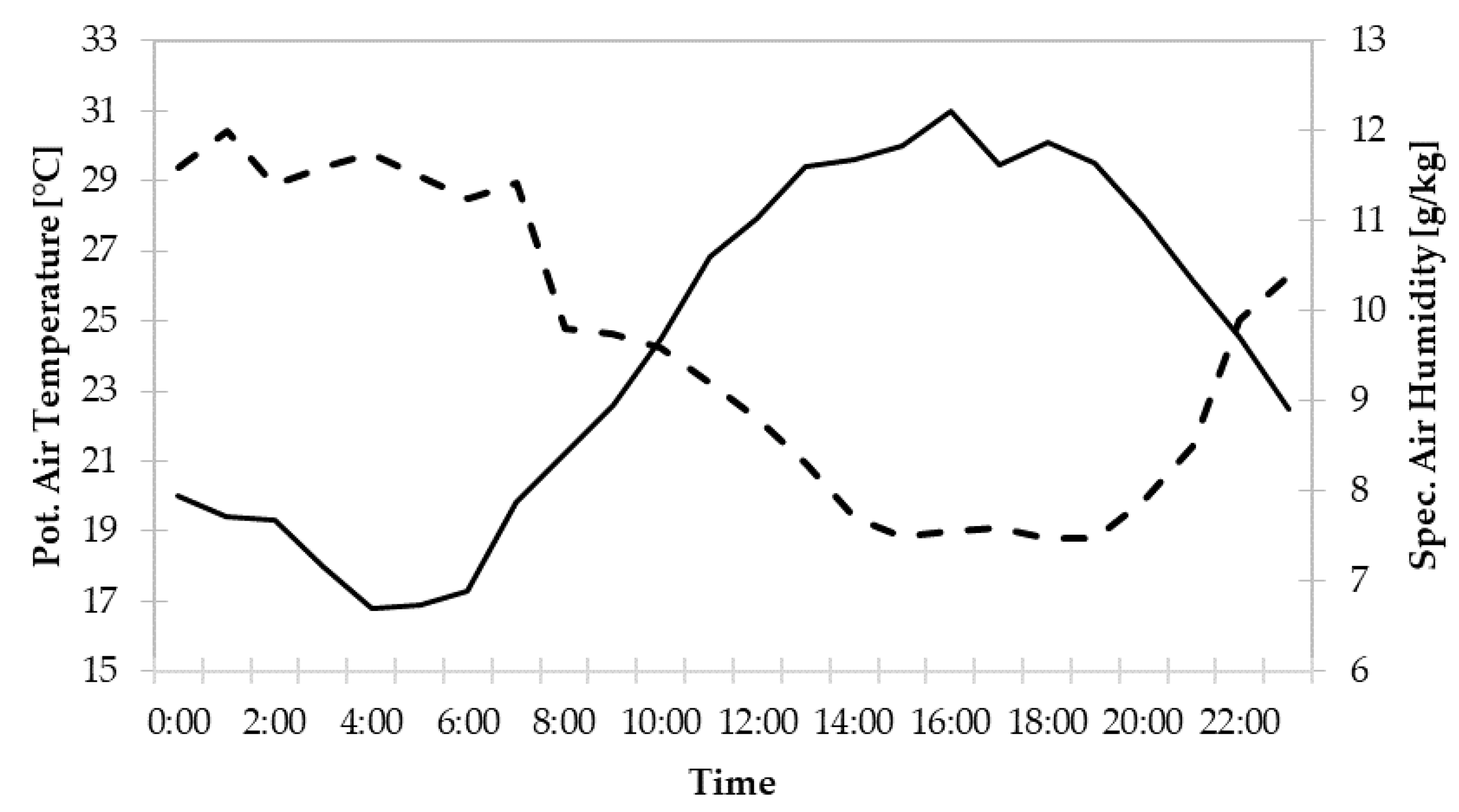
The meteorological boundary conditions were taken from an Energy Plus Weather File for Frankfurt, Germany. To resemble a hot summer day with clear sky conditions, July 7th was selected as the simulation date. The wind speed was set to 1.5 m/s in 10 m height coming from 230°. The simulation was run for 24 h. Figure 5 shows the meteorological conditions for the whole simulation period provided by the EPW-file.

4. Results and Discussion

To give an overview on the capabilities of LaStTraM, model results of the homogenous, simple inhomogeneous, and complex model areas are presented. To evaluate the performance of LaStTraM, the results of the homogeneous model area are compared against the FFP model and the K–M-model. Since no other model was available to compare the simple inhomogeneous and complex model area outputs, their results are only visualized, and their plausibility is discussed.

4.1. Evaluation of Homogeneous Model Area Results

The evaluation of the ENVI-met based footprint simulation LaStTraM with two well-known models, an analytical model and a model that is based on a Lagrangian model [9,11], demonstrates that the modeled footprints are comparable for detector heights of 3 m, 20 m, and 40 m in stable and unstable conditions despite the structural differences of the models (see Figure 6). In the unstable cases, the maximum footprint contribution ($f_{max}$) of LaStTraM tends to be higher than the other two models while the length of the footprint ($x_{max}$) tends to be slightly shorter in LaStTraM. This phenomenon featuring both an underestimation of $f_{max}$ and an overestimation of the footprint length $x_{max}$ of the FFP and K–M model was also attested by Heidbach et al., 2017 [37]. Similarly, Van de Boer et al., 2013 [38] concluded that the FFP model and two other models rather overestimated the footprint length. Regarding the distance between the detector and $f_{max}$ ($x_{max}$), LaStTraM shows very similar results compared to the FFP and K–M model with slightly shorter distances in the unstable cases and distances between the FFP and K–M models in the stable cases (see

Table 3. Crosswind distance between f_max and detector $x_{max}$.

	Detector 3 m			Detector 20 m			Detector 40 m
	LaStTraM	FFP	K–M	LaStTraM	FFP	K–M	LaStTraM	FFP	K–M
Unstable case	7 m	6 m	9 m	69 m	86 m	54 m	148 m	180 m	88 m
Stable case	10 m	16 m	6 m	269 m	226 m	92 m	598 m	690 m	193 m

).

The footprints generated by LaStTraM show a behavior that is well-known from other models: the footprint length increases with atmospheric stability while $f_{max}$ decreases. Increasing the detectors’ height leads to an increase in the footprints’ width and $x_{max}$ but decreases $f_{max}$.

Looking at the differences in $x_{max}$ between the three models, it becomes clear that LaStTraM predicts similar results to FFP (see Table 3). This stands in contrast to $f_{max}$, where LaStTraM shows more similar values to K–M.

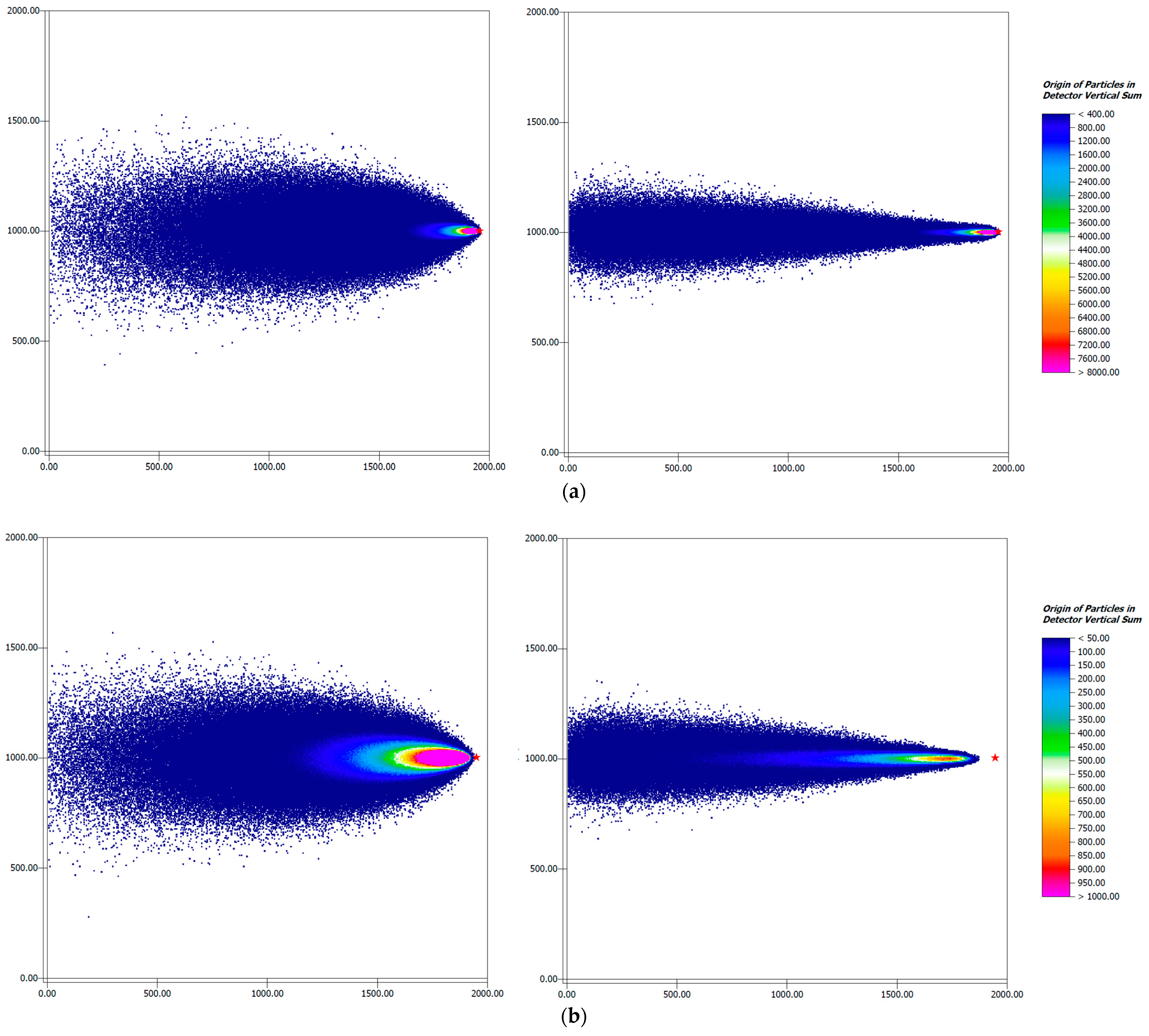
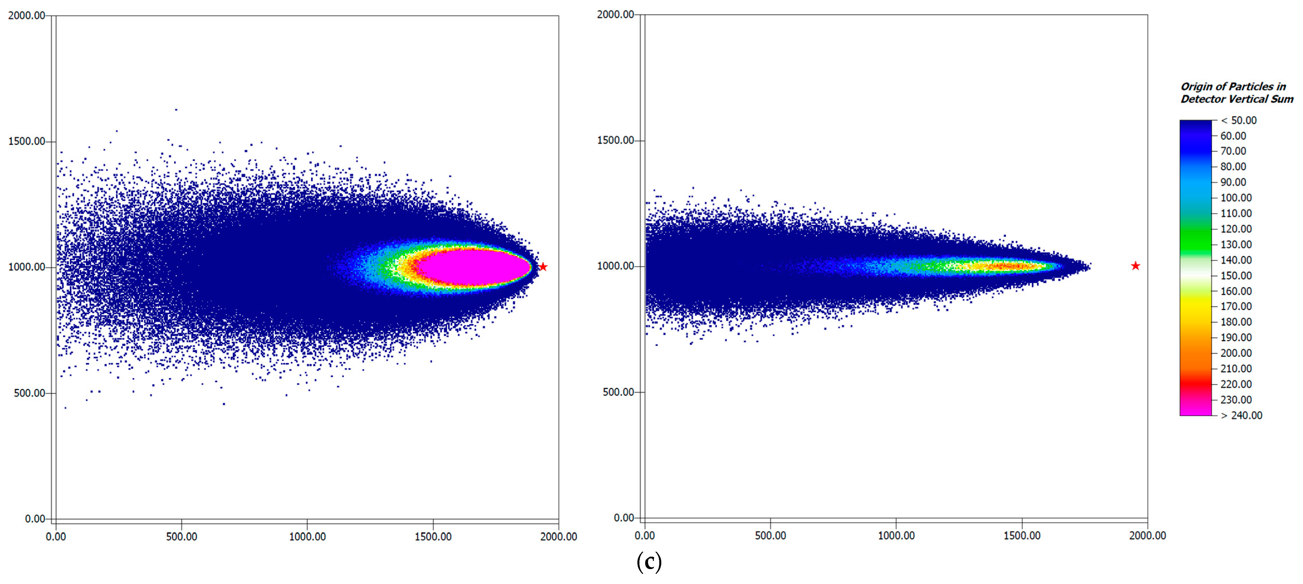
Aside from the two-dimensional crosswind integrated visualization, LaStTraM saves three-dimensional output files that can be visualized using ENVI-met’s visualization tool LEONARDO. Figure 7 shows two-dimensional representations of the three-dimensional outputs of the homogeneous model area.

The two-dimensional distribution of the footprint shows that the maximum of the three-dimensional footprint is much closer to the detector location in the unstable case than in the stable case (see Figure 7). Furthermore, the along-wind distance is increased in the unstable case compared to the stable case. In general, the footprint of the unstable case is broader due to more turbulence and thus higher atmospheric mixing during daytime.

The evaluation of the new footprint model in comparison with the established models FFP and K–M shows that LaStTraM is capable of reproducing their results. The calculated footprints resemble the results of both models and even improve the imprecisions mentioned by Heidbach et al., 2017 and Van de Boer et al. (2013) [37,38], i.e., LaStTraM most likely does not underestimate $f_{max}$ and overestimate the footprint length.

4.2. Evaluation of Simple Inhomogeneous Model Area Results

The results of the simple inhomogeneous case indicate that the tree contributes significantly differently to the footprint compared to the grass vegetation at the same distance from the detector (Figure 8). In the simulation where the detector is positioned close to the building, less particles reach the tree compared to grass cells at the same distance. This is caused by the flow induced by the building that leads to a significant updraft downwind of the tree (see Figure 9). In comparison to the grass at the same location, less particles are thus traced back to the tree from the detector close to the building.

In the simulation, where the detector is placed further downstream of the building the same effect—uplifting of flow and subsequent down-drafting due to the building—leads to more particles reaching the tree compared to the grass vegetation below the tree. Furthermore, it can be seen that despite the simple inhomogeneous model area and the Lagrangian Stochastic approach, where the particles velocity is calculated including a stochastic, random part ($P_{V_{LS}}$ in Equation (7)), the vast number of simulated particles (100 million) ensures the high symmetry of the footprint (see Figure 8).

Both footprints show greater horizontal extents than in the homogenous results. This is likely caused by the much higher turbulence induced by the complex structures in the model area. Nevertheless, with increasing distance, the number of particles from emitter cells decreases, just as in the homogeneous case.

4.3. Evaluation of Realistic Model Area Results

The results for the realistic model area confirm the general functionality of the model in complex model domains. Despite having no measurement data for this scenario, the distribution of particles shows plausible results: the vegetation closer to the detector is reached by more particles than those further away and the horizontal extent increases with increased distance from the detector (see Figure 10). Additionally, vegetation with greater vertical extent, i.e., larger trees, is more likely to be reached by the particles released from the detector. This is especially the case for the trees directly located upwind of the detector as the flow passing through them is lifted and directed upwards towards the detector’s location.

5. Conclusions

Based on the three-dimensional model outputs of the microclimate model ENVI-met, the post-processing tool LaStTraM simulates probability distributions of particles using the Lagrangian Stochastic method. Combining LaStTraM with ENVI-met should allow us to simulate flux and concentration footprints in complex urban environments.

A footprint comparison for homogenous model areas between LaStTraM and two established models shows slight deviations for the maximum footprint contribution ($f_{max}$) and the footprint length ($x_{max}$). These deviations, however, might be a result of an underestimation of $f_{max}$ and overestimation $x_{max}$ by both the FFP and K–M model as demonstrated by earlier studies [37,38]. The results of the inhomogeneous model area and the complex model area shows reasonable results where the effects of obstructions alter the particle distribution significantly. While these scenarios provided promising results, a comparison with empirical data would be needed in order to verify the accuracy of the model in complex urban areas.

The great potential of LaStTraM lies in its ensemble with ENVI-met’s averaged Navier Stokes model outputs, which should allow the study of footprints in heterogeneous and hilly environments. Our attempt to simulate a footprint in heterogeneous conditions demonstrated the capabilities of the model, i.e., incorporating three-dimensional emitters as well as the influence of obstacles on particle trajectories.

By incorporating ENVI-met’s physiological aspects of vegetation, i.e., the cell based calculation of stomatal conductance and thus transpiration, the simulation of the footprint using LaStTraM can further be improved. Footprints of different compounds can also be studied separately, depending on the variable of interest. For example, the dependency of various compounds on the flux footprint can be studied by defining individual areas/volumes that act as sources of these compounds. All results can then be visualized with the built-in ENVI -met program LEONARDO.

It was demonstrated that 100 million particles within a 2 × 2 km² model area can be modelled within a few hours on a PC. The order of magnitude of particle numbers, the model area size as well as the grid resolution are comparable to numbers reported in LES footprint studies before [16], with the essential difference that the footprint model is run in backwards mode, which means that every modelled particle (that hits a source in the model domain) influences the footprint. In contrast to a forward in time trajectory mode, the backwards mode has the advantage that the detector does not have to be unrealistically large in order to gather a sufficiently large number of particles, as demonstrated before [16].

One drawback to eddy covariance users is that the ENVI-met model cannot be run routinely for each 30 min flux average, which it has in common with all RANS and LES models. The possibility of simulating whole years with the microclimate model ENVI-met could be to split the simulations into partially overlapping timeframes, e.g., 12 simulations, one for every month of the year, including a couple of days of overlap. These could be run on 12 PCs in parallel and the overlapping results could be stitched together in the end to create a year-long simulation [39].

Regardless of the timeframe, LaStTrAM is capable of reproducing typical atmospheric conditions (unstable, stable) that will help to elucidate the origin of measured fluxes in heterogeneous environments. The LaStTraM footprint model is therefore uniquely positioned for eddy covariance studies in complex urban terrains, where the premises of analytic models are generally not met. It also can be used to analyze flux footprint problems that frequently occur in rural locations when eddy covariance towers are positioned close to forest edges or when other steep changes in roughness occur.

The present work is far from exploiting the whole potential of LaStTraM, as larger and especially more complex areas could be modelled in future studies. Furthermore, it has the potential to model the footprint of reactive gases instead of only inert particles as shown in this study. Vesala et al. (2008) highlight the potential of ensemble-averaged closure models especially for sites with complex topography and canopy heterogeneity. This includes urban sites, which are of increasing interest in surface–atmosphere exchange studies. By combining LaStTraM with ENVI-met, model areas featuring buildings, sources, vegetation, and uneven terrain can be simulated. This makes it a viable tool to calculate and analyze three-dimensional footprints in complex environments.

References

- Baldocchi, D.; Chu, H.; Reichstein, M. Inter-Annual Variability of Net and Gross Ecosystem Carbon Fluxes: A Review. Agric. For. Meteorol. 2018, 249, 520–533. [Google Scholar] [CrossRef] [Green Version]
- Chu, H.; Baldocchi, D.D.; John, R.; Wolf, S.; Reichstein, M. Fluxes All of the Time? A Primer on the Temporal Representativeness of FLUXNET. J. Geophys. Res. Biogeosci. 2017, 122, 289–307. [Google Scholar] [CrossRef]
- Konopka, J.; Heusinger, J.; Weber, S. Extensive Urban Green Roof Shows Consistent Annual Net Uptake of Carbon as Documented by 5 Years of Eddy-Covariance Flux Measurements. J. Geophys. Res. Biogeosci. 2021, 126. [Google Scholar] [CrossRef]
- Schmid, H.P. Footprint Modeling for Vegetation Atmosphere Exchange Studies: A Review and Perspective. Agric. For. Meteorol. 2002, 113, 159–183. [Google Scholar] [CrossRef]
- Vesala, T.; Kljun, N.; Rannik, U.; Rinne, J.; Sogachev, A.; Markkanen, T.; Sabelfeld, K.; Foken, T.; Leclerc, M.Y. Flux and Concentration Footprint Modelling: State of the Art. Environ. Pollut. 2008, 153, 653–666. [Google Scholar] [CrossRef]
- Leclerc, M.Y.; Foken, T. Footprints in Micrometeorology and Ecology, 1st ed.; Springer: Berlin/Heidelberg, Germany, 2014; ISBN 978-3-642-54545-0. [Google Scholar]
- Horst, T.W.; Weil, J.C. How Far Is Far Enough?: The Fetch Requirements for Micrometeorological Measurement of Surface Fluxes. J. Atmos. Ocean. Technol. 1994, 11, 1018–1025. [Google Scholar] [CrossRef] [Green Version]
- Hsieh, C.-I.; Katul, G.; Chi, T. An Approximate Analytical Model for Footprint Estimation of Scalar Fluxes in Thermally Stratified Atmospheric Flows. Adv. Water Resour. 2000, 23, 765–772. [Google Scholar] [CrossRef]
- Kljun, N.; Calanca, P.; Rotach, M.W.; Schmid, H.P. A Simple Two-Dimensional Parameterisation for Flux Footprint Prediction (FFP). Geosci. Model Dev. 2015, 8, 3695–3713. [Google Scholar] [CrossRef] [Green Version]
- Kljun, N.; Calanca, P.; Rotach, M.W.; Schmid, H.P. A Simple Parameterisation for Flux Footprint Predictions. Bound. Layer Meteorol. 2004, 112, 503–523. [Google Scholar] [CrossRef]
- Kormann, R.; Meixner, F.X. An Analytical Footprint Model For Non-Neutral Stratification. Bound. Layer Meteorol. 2001, 99, 207–224. [Google Scholar] [CrossRef]
- Schuepp, P.H.; Leclerc, M.Y.; MacPherson, J.I.; Desjardins, R.L. Footprint Prediction of Scalar Fluxes from Analytical Solutions of the Diffusion Equation. Bound. Layer Meteorol. 1990, 50, 355–373. [Google Scholar] [CrossRef]
- Horst, T.W.; Weil, J.C. Footprint Estimation for Scalar Flux Measurements in the Atmospheric Surface Layer. Bound. Layer Meteorol. 1992, 59, 279–296. [Google Scholar] [CrossRef]
- Kljun, N.; Rotach, M.W.; Schmid, H.P. A Three-Dimensional Backward Lagrangian Footprint Model for a Wide Range of Boundary-Layer Stratifications. Bound. Layer Meteorol. 2002, 103, 205–226. [Google Scholar] [CrossRef]
- Cai, X.; Leclerc, M.Y. Forward-in-Time and Backward-in-Time Dispersion in the Convective Boundary Layer: The Concentration Footprint. Bound. Layer Meteorol. 2007, 123, 201–218. [Google Scholar] [CrossRef]
- Hellsten, A.; Luukkonen, S.-M.; Steinfeld, G.; Kanani-Sühring, F.; Markkanen, T.; Järvi, L.; Lento, J.; Vesala, T.; Raasch, S. Footprint Evaluation for Flux and Concentration Measurements for an Urban-Like Canopy with Coupled Lagrangian Stochastic and Large-Eddy Simulation Models. Bound. Layer Meteorol. 2015, 157, 191–217. [Google Scholar] [CrossRef]
- Leclerc, M.Y.; Shen, S.; Lamb, B. Observations and Large-Eddy Simulation Modeling of Footprints in the Lower Convective Boundary Layer. J. Geophys. Res. Atmos. 1997, 102, 9323–9334. [Google Scholar] [CrossRef]
- Kurbanmuradov, O.; Levykin, A.; Rannik, U.; Sabelfeld, K.; Vesala, T. Stochastic Lagrangian Footprint Calculations over a Surface with an Abrupt Change of Roughness Height. Mt. Carlo Methods Appl. 2003, 9. [Google Scholar] [CrossRef]
- Luhar, A.K.; Rao, K.S. Source Footprint Analysis for Scalar Fluxes Measured in Flows over an Inhomogeneous Surface. In Air Pollution Modeling and Its Application X; Gryning, S.-E., Millán, M.M., Eds.; Springer: Boston, MA, USA, 1994; pp. 315–323. ISBN 978-1-4613-5734-6. [Google Scholar]
- Sogachev, A.; Menzhulin, G.V.; Heimann, M.; Lloyd, J. A Simple Three-Dimensional Canopy—Planetary Boundary Layer Simulation Model for Scalar Concentrations and Fluxes. Tellus B 2002, 54, 784–819. [Google Scholar] [CrossRef]
- Bruse, M.; Fleer, H. Simulating Surface Plant Air Interactions inside Urban Environments with a Three Dimensional Numerical Model. Environ. Model. Softw. 1998, 13, 373–384. [Google Scholar] [CrossRef]
- Jacobs, C.M.J. Direct Impact of Atmospheric CO2 Enrichment on Regional Transpiration. Ph.D. Thesis, Agricultural University Wageningen, Wageningen, The Netherlands, 1994. [Google Scholar]
- Bruse, M. ENVI-Met Implementation of the Jacobs A-Gs Model to Calculate the Stomata Conductance; Bochum, Germany. 2004. Available online: http://www.envi-met.net/documents/new_a_gs.pdf (accessed on 28 July 2021).
- Simon, H.; Lindén, J.; Hoffmann, D.; Braun, P.; Bruse, M.; Esper, J. Modeling Transpiration and Leaf Temperature of Urban Trees—A Case Study Evaluating the Microclimate Model ENVI-Met against Measurement Data. Landsc. Urban Plan. 2018, 174, 33–40. [Google Scholar] [CrossRef]
- Bruse, M. Die Auswirkungen Kleinskaliger Umweltgestaltung auf das Mikroklima. Entwicklung des Prognostischen Numerischen Modells ENVI-met zur Simulation der Wind-, Temperatur- und Feuchteverteilung in Städtischen Strukturen. Ph.D. Thesis, Ruhr-University Bochum, Bochum, Germany, 1999. [Google Scholar]
- Simon, H. Modeling Urban Microclimate: Development, Implementation and Evaluation of New and Improved Calculation Methods for the Urban Microclimate Model ENVI-Met. Ph.D. Thesis, Johannes Gutenberg-University Mainz, Mainz, Germany, 2016. [Google Scholar]
- Huttner, S. Further Development and Application of the 3D Microclimate Simulation ENVI-Met. Ph.D. Thesis, Johannes Gutenberg-University Mainz, Mainz, Germany, 2012. [Google Scholar]
- Ali-Toudert, F. Dependence of Outdoor Thermal Comfort on Street Design in Hot and Dry Climate. Ph.D. Thesis, Albert-Ludwigs-Universität Freiburg, Breisgau, Germany, 2005. [Google Scholar]
- Shepard, D. A Two-Dimensional Interpolation Function for Irregularly-Spaced Data. In Proceedings of the 1968 23rd ACM National Conference, New York, NY, USA, 27–29 August 1968; ACM Press: New York, NY, USA, 1968; pp. 517–524. [Google Scholar]
- Weil, J.C.; Sullivan, P.P.; Moeng, C.-H. The Use of Large-Eddy Simulations in Lagrangian Particle Dispersion Models. J. Atmos. Sci. 2004, 61, 2877–2887. [Google Scholar] [CrossRef]
- Thomson, D.J. Criteria for the Selection of Stochastic Models of Particle Trajectories in Turbulent Flows. J. Fluid Mech. 1987, 180, 529–556. [Google Scholar] [CrossRef]
- Maronga, B.; Gryschka, M.; Heinze, R.; Hoffmann, F.; Kanani-Sühring, F.; Keck, M.; Ketelsen, K.; Letzel, M.O.; Sühring, M.; Raasch, S. The Parallelized Large-Eddy Simulation Model (PALM) Version 4.0 for Atmospheric and Oceanic Flows: Model Formulation, Recent Developments, and Future Perspectives. Geosci. Model Dev. 2015, 8, 2515–2551. [Google Scholar] [CrossRef] [Green Version]
- Steinfeld, G.; Raasch, S.; Markkanen, T. Footprints in Homogeneously and Heterogeneously Driven Boundary Layers Derived from a Lagrangian Stochastic Particle Model Embedded into Large-Eddy Simulation. Bound. Layer Meteorol. 2008, 129, 225–248. [Google Scholar] [CrossRef]
- Wilson, J.D.; Sawford, B.L. Review of Lagrangian Stochastic Models for Trajectories in the Turbulent Atmosphere. Bound. Layer Meteorol. 1996, 78, 191–210. [Google Scholar] [CrossRef]
- Flesch, T.K. The Footprint for Flux Measurements, from Backward Lagrangian Stochastic Models. Bound. Layer Meteorol. 1996, 78, 399–404. [Google Scholar] [CrossRef]
- Markkanen, T.; Steinfeld, G.; Kljun, N.; Raasch, S.; Foken, T. Comparison of Conventional Lagrangian Stochastic Footprint Models against LES Driven Footprint Estimates. Atmos. Chem. Phys. 2015, 9, 5575–5586. [Google Scholar] [CrossRef] [Green Version]
- Heidbach, K.; Schmid, H.P.; Mauder, M. Experimental Evaluation of Flux Footprint Models. Agric. For. Meteorol. 2017, 246, 142–153. [Google Scholar] [CrossRef] [Green Version]
- van de Boer, A.; Moene, A.F.; Schüttemeyer, D.; Graf, A. Sensitivity and Uncertainty of Analytical Footprint Models According to a Combined Natural Tracer and Ensemble Approach. Agric. For. Meteorol. 2013, 169, 1–11. [Google Scholar] [CrossRef]
- Simon, H.; Bruse, M.; Cramer, L.; Sinsel, T. Improving Building Performance Simulation Boundary Conditions. In Proceedings of the 35th International Conference on Passive and Low Energy Architecture, A Coruña, Spain, 1–3 September 2020; Volume 1, p. 6. [Google Scholar]