Statistical Downscaling of Urban-scale Air Temperatures Using an Analog Model Output Statistics Technique

Abstract

This study was conducted to evaluate the suitability of an analog model output statistics (MOS) downscaling technique for urban-scale meteorology research and compares this MOS-Analog technique with the sliding window technique. We downscaled air temperatures forecasted for the Seoul metropolitan area from 1.5 km resolution (using data from the Unified Model-Local Data Assimilation and Prediction System, UM-LDAPS) to 25 m resolution using the analog MOS technique described in the paper. The support vector machine (SVM) technique was employed for empirical computational modeling, using urban surface parameters calculated using the Climate Analysis Seoul (CAS) workbench and automated weather station (AWS) observational data as training data. The comparison of the downscaled prediction results with the AWS observations for the periods of July/August 2016 and 2017 resulted in a lower root mean square error (RMSE) and higher correlation coefficients (CC) than those obtained for the LDAPS prediction results. The prediction performance was also stable for September, during which precipitation episodes and seasonal fluctuations occurred. The results of this study demonstrate that the proposed technique, which overcomes the limitations of the sliding window technique, is applicable to urban-scale meteorology research and potentially applicable other areas.

1. Introduction

Major weather events are predicted on global or regional scales using global climate models, also known as general circulation models (GCMs) or regional climate models (RCMs). However, most weather disasters occur at local or microscale levels [1,2]. Urban-scale weather phenomena, such as heat islands, precipitation variations, and air quality changes, exhibit spatial differences depending on urban surface characteristics, such as urban structures and land cover characteristics [3].

With the growing demand for high-resolution spatiotemporal weather prediction data in the field of urban-scale climate change adaptation and response [4,5,6,7], downscaling is increasingly being used as a method to handle detailed spatiotemporal meteorological information. Two techniques are used. The first type is dynamic downscaling, which is applied to a regional numerical model to obtain a higher spatial resolution than is obtained with a GCM. GCM-based downscaled local and urban-scale weather prediction models coupled with dynamic downscaling techniques are now available. However, dynamic downscaling models are prone to systematic error on a regional scale. They are also limited in their ability to reflect regional characteristics because of the low-resolution topographic data used [8,9,10,11]. In the field of urban-scale climate prediction, which requires building-level resolution, it is particularly difficult to use dynamically downscaled data [12].

The second type of technique is statistical downscaling, which uses statistical relations between numerically predicted weather data and observed data to correct the bias in the former. Significant reduction in bias through the use of statistical downscaling has been reported [13,14,15,16].

There are many ways to analyze numerically predicted weather data objectively. The perfect prog method (PPM) and model output statistics (MOS) are typical statistical downscaling methods [17]. MOS produces predictands, not predictors. The predictors are produced by the GCM/RCM and are inputs to the MOS models. Furthermore, MOS models cannot explain systematic errors, but they can correct for them, which is a way to calibrate the forecasts. The MOS downscaling technique continues to be upgraded and is made more amenable to practical uses as the performance of numerical weather prediction models improves [18]. MOS-based models include linear regression and analog models, with which past records are examined for weather conditions similar to the current one. Many recent research efforts have been devoted to machine learning-based statistical downscaling applications, including linear/nonlinear relationships [19,20]. Notably, studies in which machine learning has been compared with other approaches have consistently found that the former outperforms the latter [21]. In addition, among the machine-learning methods available, SVM models have been reported in various studies to be applicable to the spatial downscaling of several factors. SVM regression models also allow easy manipulation and require only low-level calculations, which makes them desirable for use in a variety of fields [22,23].

In a recent study, spatial downscaling from a resolution of 1.5 km to 25 m was accomplished by applying machine learning to the local data assimilation and prediction system (LDAPS) of the unified model (UM), an air temperature forecast (spatial resolution: 1.5 km) that receives its boundary fields from the global data assimilation and prediction system (GDAPS) [24]. In that study, the latest temperature trends in the prediction model were reflected using a training dataset consisting of temperature data for the last 30 days and a sliding window technique to calculate the maximum and minimum temperatures of the subsequent day. The overall summer temperature prediction accuracy was found to be enhanced, but sudden meteorological changes, such as rainfall events, were overestimated.

Statistical downscaling of urban-scale temperatures requires not only a high-resolution numerical weather prediction model, but also the application of a statistical downscaling technique to reflect the actual temperature profile of a complex urban structure to the greatest extent possible, as shown in the aforementioned study. Turco et al. [25] downscaled RCM-computed complex terrain precipitation data using an analog technique based on a MOS technique (hereinafter MOS-Analog), demonstrating its potential to yield stable and improved downscaling outputs [25]. In this study, we performed statistical downscaling of temperature prediction data to high-resolution data by applying the MOS-Analog technique to complex urban-scale LDAPS prediction results and evaluated the operational suitability of its results.

2. Materials and Methods

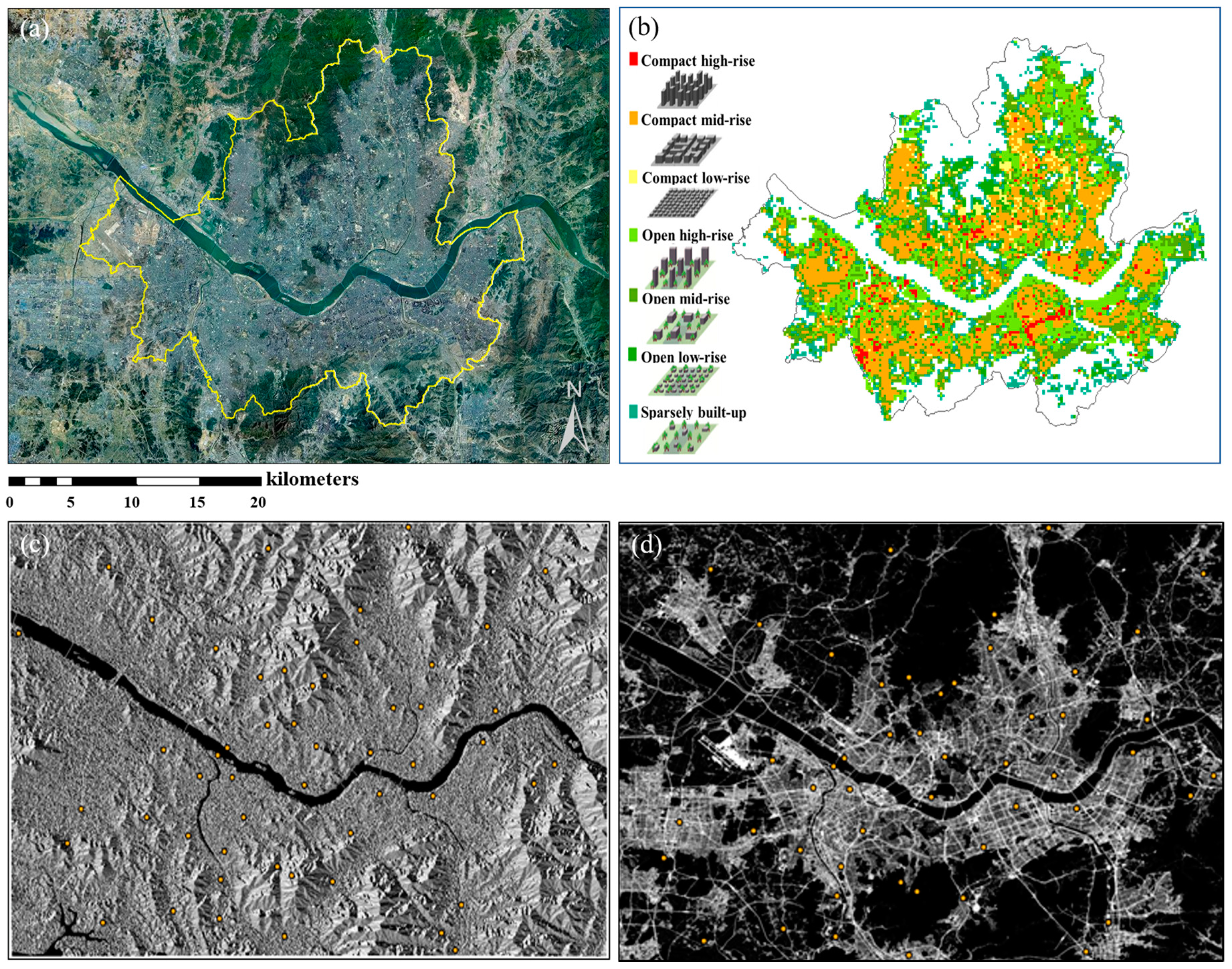
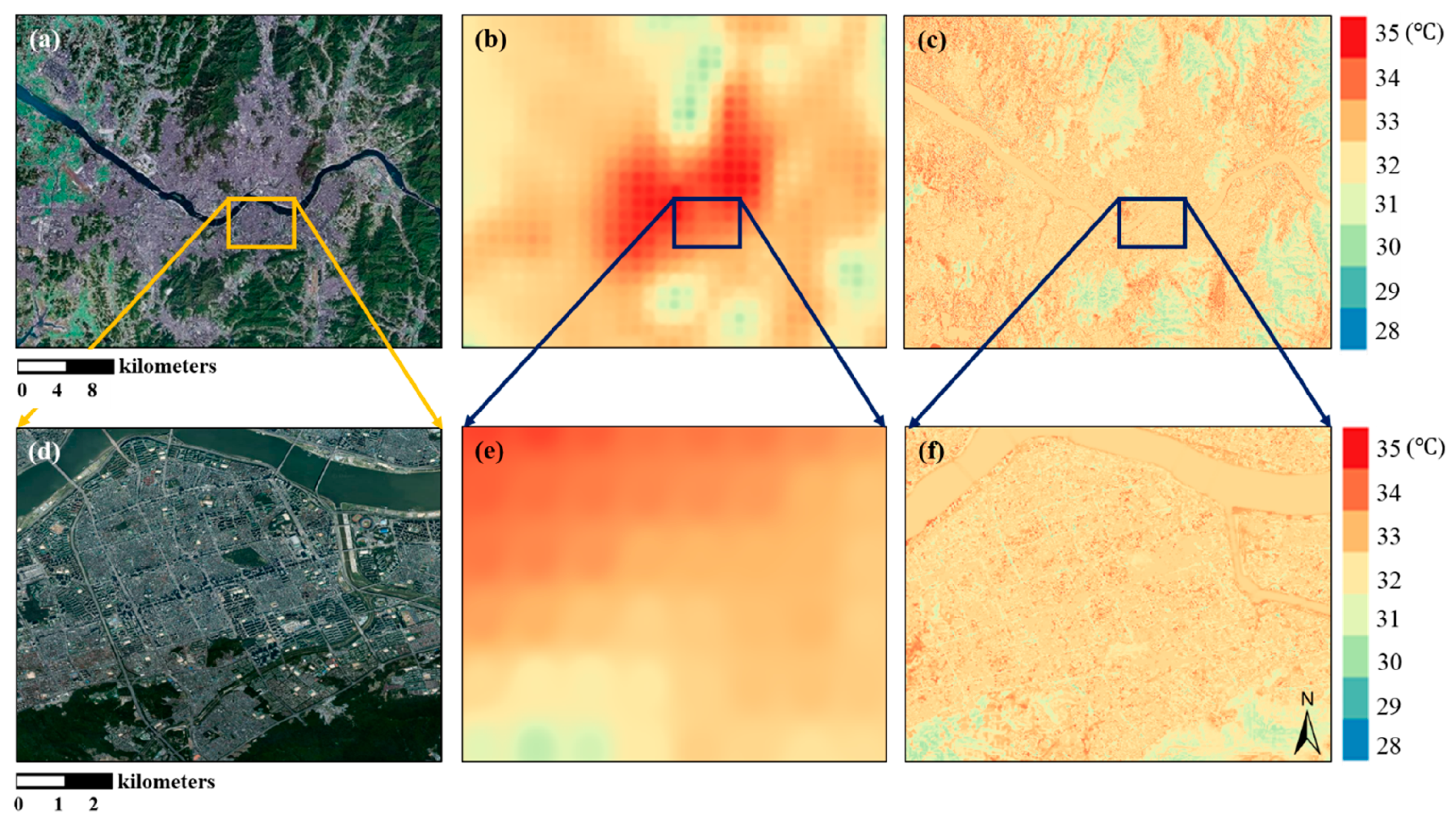
2.1. Study Region

The study region, Seoul (605${\mathrm{km}}^2$; 37°25′–37°41′ N, 126°45′–127°11′ E), is the capital city of and largest metropolis in the Republic of Korea, in Northeast Asia. The Han River runs through the center of Seoul, which lies in a basin encircled by mountains (Figure 1a). Seoul is characterized by tall buildings and a high population density, with over 9.7 million people (i.e., 18% of the population of Korea), living in an area that accounts for only 0.6% of the country, making it the most densely populated of Organisation for Economic Co-operation and Development (OECD) cities. According to the local climate zone (LCZ) types proposed by Steward and Oke [26], which describe urban landscapes based on climatic characteristics that depend on land cover and building configuration factors, Seoul is largely characterized by compact mid-rise building clusters, interspersed with high-rise commercial buildings and low-rise residential quarters, with its land cover consisting predominantly of impervious surfaces (Figure 1b). Its flat surfaces are filled with buildings of various shapes and with streets (Figure 1c,d). The number of heat days (those with daily maximum temperatures above 33 °C) in Seoul between 2010 and 2016 (Seoul Weather Station, AWS #108, Korea Meteorological Administration) and the number of patients diagnosed with heat-related illnesses (National Health Insurance Service) suggest that both the number of heat days and the number of patients with heat-related illnesses in the Seoul Metropolitan Area are on the rise (Figure 2). With a high population ratio exposed to the heat island phenomenon, there is a compelling need to establish high-resolution spatiotemporal weather prediction data for use in the efficient management of climate change adaptation and response.

2.2. Numerical Weather Prediction Models

The LDAPS was configured for high-resolution weather prediction over the Korean peninsula and surrounding waters (

Table 1. Local Data Assimilation and Prediction System (LDAPS) variables used for downscaling of air temperature.

Label	Description	Units
TMP	Air temperature 1.5 m above the ground	$\mathrm{K}$
NCPCP	Total precipitation	$\mathrm{kg}/{\mathrm{m}}^2$
RH	Relative humidity 1.5 m above the ground	$\%$
TCAR	Total cloud cover (random overlap)	$\%$
UGRD	10-m U wind component	$\mathrm{m}/\mathrm{s}$
VGRD	10-m V wind component	$\mathrm{m}/\mathrm{s}$

). Its spatial resolution is 1.5 km, and it consists of 70 vertical levels up to 40 km. With a horizontal grid spacing of 1.5 km, starting from the lower left corner (121.834° E, 32.257° N), LDAPS has 602 grid cells in the x-direction (East–West) and 781 grid cells in the y-direction (North–South). It receives boundary fields at 3-h intervals from the GDAPS, which has a horizontal grid spacing of 17 km, and performs weather prediction eight times a day (00:00, 06:00, 12:00, and 18:00 Coordinated Universal Time (UTC): 36-h prediction; 03:00, 09:00, 15:00, and 21:00 UTC: 3-h prediction). The system is operated as a self-analyzing prediction cycle system based on a three-dimensional variational (3DVAR) data assimilation system. There are two types of LDAPS-computed data: Isobaric surface data (seven parameters in the range of 1000–50 hPa) and grid surface data (78 parameters; Figure 3a) [27].

The data collection period considered in the present study was 2015–2017. The available 12 h prediction data (00:00, 06:00, 12:00, and 18:00 UTC: h000–h011) were selected from the LDAPS 36 h prediction data (00:00, 06:00, 12:00, and 18:00 UTC: h000–h036) for use in this study. The data for the time period between h000 and h005 were used as the model training data, and those for the time period between h006 and h011 were used as prediction data. Thus, four forecasting periods per day were considered (denoted 00:00, 06:00, 12:00, and 18:00 UTC, where 00:00 UTC refers to the period from 06:00 to 11:00, 06 UTC refers to the period from 12:00 to 17:00, 12 UTC refers to the period from 18:00 to 23:00, and 18:00 UTC refers to the period from 00:00 to 05:00).

The air temperature prediction dataset at the same spatial resolution is an essential component of spatial resolution downscaling to 25 m spatial resolution. We interpolated the air temperature forecast for the Seoul Metropolitan Area (50 km × 40 km; Figure 3b) from the LDAPS prediction results (Figure 3a) to 25 m grid resolution using the inverse distance weighting (IDW) interpolation method.

2.3. Urban Surface Parameters

We calculated 25 m resolution urban surface parameters using the Climate Analysis Seoul (CAS) workbench. The CAS workbench is a model suitable for computing topographic and land cover parameters and analyzing microclimate (heat and wind) spatial distribution profiles [28,29,30]. First, we parameterized the three-dimensional (3-D) topographical structure from a digital terrain model (DTM) and digital surface model (DSM) and computed 3-D topographic parameters, such as the hollow depth, aspect ratio, dzdx, dzdy, and slope length. We then parameterized land cover information from land cover (LC) data and computed the values of parameters related to horizontal characteristics such as areal type, complete surface area ratio, fractional coverage, building height, and vegetation height.

Table 2. Urban surface parameters used for downscaling of air temperature.

Label	Description	Units
Aspect	Aspect angle	$\mathrm{deg}$
CSAR	Complete surface aspect ratios derived from BH	$\%$
dzdx	Topographic gradient in the x-direction	$\mathrm{m}/\mathrm{m}$
dzdy	Topographic gradient in the y-direction	$\mathrm{m}/\mathrm{m}$
Building height	Building height derived from airborne LiDAR	$\mathrm{m}$
Vegetation height	Vegetation height derived from airborne LiDAR	$\mathrm{m}$
Hollow depth	Hollow depth by building and terrain	$\mathrm{m}$
Slope	Slope angle	$\mathrm{deg}$
BS area	Fractional coverage of building surfaces	$\%$
US area	Fractional coverage of impervious surfaces	$\%$
TV area	Fractional coverage of tall vegetated surfaces	$\%$
VS area	Fractional coverage of vegetated surfaces	$\%$
WS	Fractional coverage of water surfaces	$\%$
Z	Sea level	$\mathrm{m}$
Areal type	Forms of land cover	-
BHBS	Building volume	-

lists the CAS-computed urban surface parameters (Table 2).

2.4. AWS data

We used 3-y (2015–2017) observation data from 50 AWSs operated by the Korea Meteorological Administration in the Seoul Metropolitan Area. The temperature data from the AWSs in the city center clearly reflected the influence of heat generated in relation to urban surface characteristics and physical structures in addition to that from mesoscale phenomena. On a related note, Yi et al. [31] confirmed a high correlation between the quantitative distribution of human-made structures, such as buildings and streets, and thermal features identified as a result of microclimatic analysis.

AWS data were used for two purposes. First, they were used as predictands of the training model to obtain an empirical equation that could be used to estimate correlations between surface parameters and observed air temperatures. For example, building and street fractions are different from one AWS to another, and the corresponding data for each AWS are used as representative fractional values of that AWS (Figure 4). Second, AWS data were used to test the urban-scale air temperature prediction accuracy during various weather episodes (e.g., summer, heatwaves (more than two days with maximum temperatures above 33 °C), tropical nights (more than two days with minimum temperatures above 25 °C), precipitation events, and seasonal variations).

2.5. MOS-Analog Technique

The MOS-Analog technique is a weather prediction method that uses statistical relationships between observational data and numerical prediction model outputs [32]. It can correct for systematic errors in numerical weather prediction models and generate predictands for a specific point. Due to the advantages that the MOS-Analog technique offers in improving the outputs of numerical weather prediction models, it has been continuously developed and made more amenable for use in practical applications [33,34].

An analog technique is based on the hypothesis that “analog” atmospheric patterns (predictors) induce “analog” local effects (predictands) [35,36]. The days for which data are extracted based on similar atmospheric spatial patterns in a given set of forecasts and past case histories are called “analog days.” In this study, Euclidean distances were calculated, and the Euclidean distances were defined in analogous order from the closest to the third past case. This is one of the most widely used downscaling techniques in applications in a variety of fields [37,38,39,40].

The MOS-Analog technique proposed by Turco [25,41] has demonstrated a potential for improving prediction performance for average and extreme precipitation values in topographically complex terrains through its application to RCM results [41].

2.6. Support Vector Machine

In this study, a support vector machine (SVM) was used to search for a statistical equation linking the data from the observed and numerical prediction models. A support vector machine (SVM) is a machine learning algorithm for regression analysis or data classification, implemented by deriving specific characteristics or patterns in inter-data relationships [42]. An SVM permits the identification of factors that influence learning in a relatively simple way, with adjustment of only a small number of parameters. Furthermore, compared to artificial neural networks, less over-fitting occurs, and SVMs offer the additional benefit of being simple to use. SVMs are used in a wide variety of fields, from bioinformatics to astrophysics. We implemented an SVM regression model using epsilon regression, based on the kernel function from the kernlab package [43].

For a given data set ${\left\{\left(x_i,y_i\right)\right\}}_i^n$, the SVM regression model employed in this study uses Equation (1) below to determine the regression function $f\left(x\right)$ that optimally approximates a given y value:

$$f\left(x\right)={\omega }^{T}x+b$$

(1)

Here, $\omega$ is the weighting vector and $b$ is a constant. The $\omega$ and $b$ in Equation (1) can be estimated via conversion to an optimization problem, as shown in Equation (2).

$$\underset{\varpi ,b,\xi ,{\xi }^{*}}{\min }:R_{reg}\left(f\right)=\frac{1}{2}{\varpi }^T\varpi +c{\displaystyle {\displaystyle \sum }_{i=1}^l}{\xi }_i+c{\displaystyle {\displaystyle \sum }_{i=1}^l}{\xi }_i^{*}$$

(2)

$$\mathrm{subject}\mathrm{to}\{\begin{array}{c}{\varpi }^T\varphi \left(x_i\right)+b-z_i\le ϵ+{\xi }_i\\ z_i-{\varpi }^T\varphi \left(x_i\right)-b\le ϵ+{\xi }_i^{*}\\ {\xi }_i,{\xi }_i^{*}\ge 0,i=1,\dots ,l.\end{array}$$

Here, $\frac{1}{2}{\varpi }^T\varpi$ is a normalization term that controls the balance between complexity and accuracy in regression models; $c$ is a normalized constant for the balance between empirical risk and the normalization term, in which an increase in $c$ represents an increase in the relative proportion of empirical error with respect to the total error; $ϵ$ represents the Epsilon tube, which indicates the range of permissible errors, and a value of $ϵ$ that is too small causes overfitting of the regression model.

Application of the Lagrangian multiplier and the Karush–Kuhn–Tucker conditions to Equation (2) results in a common form of the SVM regression model in Equation (1), as shown in Equation (3).

$$f\left(x,\alpha ,{\alpha }^{*}\right)={\displaystyle {\displaystyle \sum }_{i=1}^n}\left({\alpha }_i-{\alpha }_i^{*}\right)K\left(x_i,x_j\right)+b$$

(3)

In Equation (4), $K\left(x_i,x_j\right)$ is defined as a radial basis function (RBF) kernel function that treats the training data samples as internal representatives and effectively identifies the nonlinear correlation among the samples.

$$K\left(x_i,x_j\right)=\varphi \left(x_i\right)\varphi \left(x_j\right)=\exp (-\frac{{\Vert x_i-x_j\Vert }^2}{2{\sigma }^2})$$

(4)

2.7. Computation System

In this study, we applied the MOS-Analog technique to air temperature forecasts with 1.5-km resolution (LDAPS) for the Seoul metropolitan area and downscaled it to 25 m resolution using CAS-computed urban surface parameters and AWS observation data as training data and the SVM machine learning method as an empirical computational model. We named this process the urban meteorological information system (UMIS). The UMIS output computation process consists of five major steps.

The LDAPS domain was selected to reflect the local meteorological patterns of the study region. For this study, we selected the Seoul metropolitan area (Figure 1) as the study area.

Second, Euclidean distances were calculated using LDAPS grid surface prediction parameters (TMP, NCPCP, RH, TCAR, UGRD, and NS VGRD) to search for analog days for the Seoul metropolitan area. Considering the seasonal and temporal patterns of the forecast period, the differences in month and time were limited to 1 month and 2 h, respectively.

Let $L\left(t\right)$ in Equation (5) be the predictor of the LDAPS forecast time series:

$$L\left(t\right)=\left[L_1\left(t\right),\dots ,L_n\left(t\right)\right]$$

(5)

Let $A\left(t\right)$ in Equation (6) be the prediction parameter of the LDAPS forecast results:

$$A\left(t\right)=\left[A_1\left(t\right),\dots ,A_n\left(t\right)\right]$$

(6)

where $n$ is the number of grid points $\left(n=1,\dots ,N\right)$ and $m$ is the number of predictors.

Accordingly, the Euclidean distance in the MOS-Analog technique can be defined, as shown in Equation (7):

$$D={\displaystyle {\displaystyle \sum }_{j=1}^m}{\displaystyle {\displaystyle \sum }_{i=1}^n}{\alpha }_j\left[{\left(L_{j,i}\left(t\right)-A_{j,i}\left(t\right)\right)}^2\right]$$

(7)

where ${\alpha }_j$ is the weight of each prediction parameter. The weight is empirically calculated and applied in a manner such that all parameters can explain the parameter of interest, i.e., the temperature, well.

Third, the first three analog days with the smallest Euclidean distances are set as the predictands. There were other analog-day candidates, but these three analog days outperformed them and were found to be the most stable.

Fourth, the observed data for the selected analog days were used as training data, along with LDAPS-predicted air temperature data and AWS urban surface characteristics data, and an empirical equation was derived based on SVM machine learning.

Fifth, the empirical equation was applied to the input parameters, and the air temperature at 25 m resolution was estimated.

3. Results and Discussion

3.1. Extraction and Computation of Analog Days

In this study, August 4, 2017, 06.00 (UTC) was selected as a prediction case from among the dates of the validation period (July and August 2016 and 2017, every hour between 00:00 and 23:00). The MOS technique was then applied to the LDAPS data based on site operations. The analog days corresponding to the prediction parameters of the LDAPS for the prediction case were estimated and their similarity with the prediction case was examined using the AWS observation data.

The ranks, according to Euclidean distance, calculated using the parameters of the prediction case and the previous cases, were plotted against the RMSE values for the AWS data (Figure 5a). As the rank according to the Euclidean distance decreased, the RMSE value for the observed temperatures of the prediction and previous cases increased, with CC = 0.65 indicating a positive correlation coefficient (Figure 5a). In addition, the previous cases were examined after filtering based on the conditioning of each parameter: Temperature (b), wind (c), and relative humidity (d) (Figure 5). When the Euclidean distances among the meteorological prediction parameters were filtered based on the filtering criteria, the orange parts were selected, and their removal led to a reduction in the RMSE values of the observed temperature between the prediction case and the previous cases from 3.76 °C to 1.60 °C, with a slight increase in correlation coefficient from 0.65 to 0.69 (Figure 5b). When the filtering conditions for the wind velocity prediction parameters were also considered, the red parts were selected; their removal led to a reduction in RMSE from 1.60 °C to 1.50 °C, with an increase in the correlation coefficient from 0.69 to 0.71 (Figure 5c). When the filtering conditions for the relative humidity prediction parameters were also considered, the green parts were selected, and removing these parts led to a reduction in RMSE from 1.50 °C to 1.23 °C and a slight decrease in the correlation coefficient from 0.71 to 0.70. These results indicate that the greater the number of parameters considered and combined for filtering is, the higher the agreement is between the analog days and the atmospheric patterns of the prediction case (Figure 5b–d). The analog days estimated from the rank, according to the Euclidean distance, calculated using various prediction parameters, were identical to the days obtained by conditioning each prediction parameter for filtering. Figure 5 presents the results that explain the possibility of estimating analog days from the Euclidean distance based on the meteorological prediction parameters (Figure 5a), as well as the reason for considering various other meteorological conditions in addition to temperature when examining similarities among temperatures (Figure 5b–d).

In this study, the analog days with the closest Euclidean distances to those from the ten closest previous cases were extracted. The training data were established by combining the data for the three closest previous cases (Figure 6). The following dates were selected as the analog dates: August 4, 2017, 05.00 (UTC); August 10, 2016, 06.00 (UTC); and August 18, 2016, 04.00 (UTC). The validation results based on the AWS data yielded RMSE values of 0.8 °C, 1.19 °C, and 0.84 °C, respectively, with correlation coefficients of 0.83, 0.55, and 0.7, respectively. These results indicate that the selection of atmospheric patterns was similar to the temperature distribution of the prediction case (Figure 7). Compared to the LDAPS data for temperature prediction, with an RMSE of 1.43 °C and correlation coefficient of 0.23, the data for the analog dates yielded results for the predictands that improved the accuracy of the LDAPS prediction (Figure 6). The results of the improvement in the LDAPS accuracy, based on the analog dates estimated for the entire validation period, are described in Section 3.5.

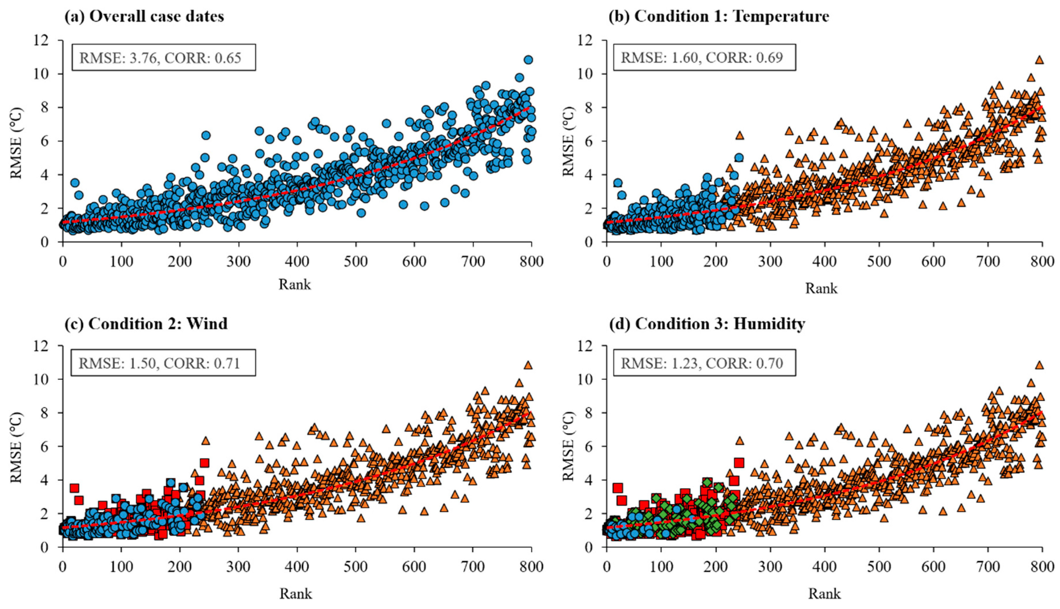
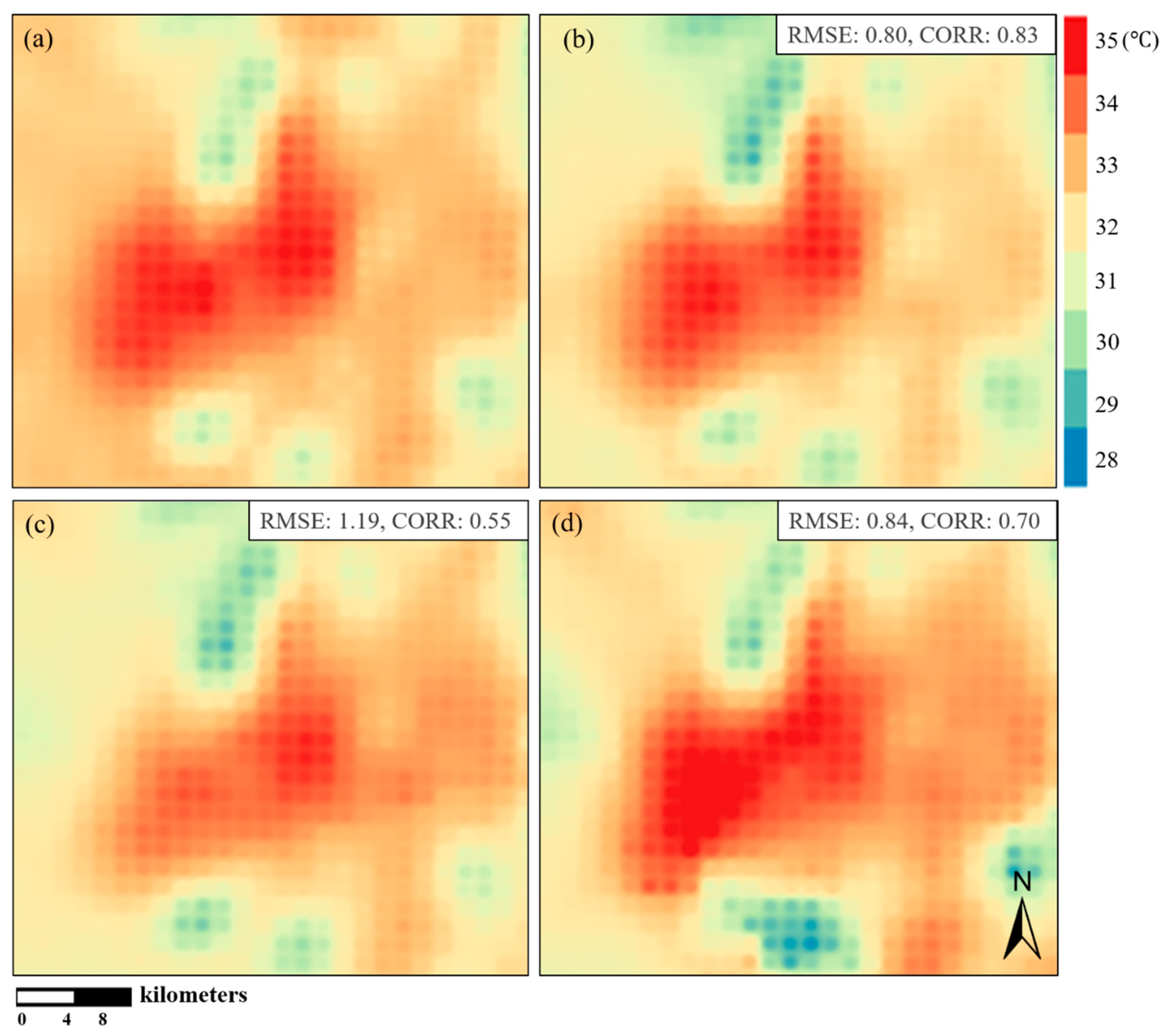
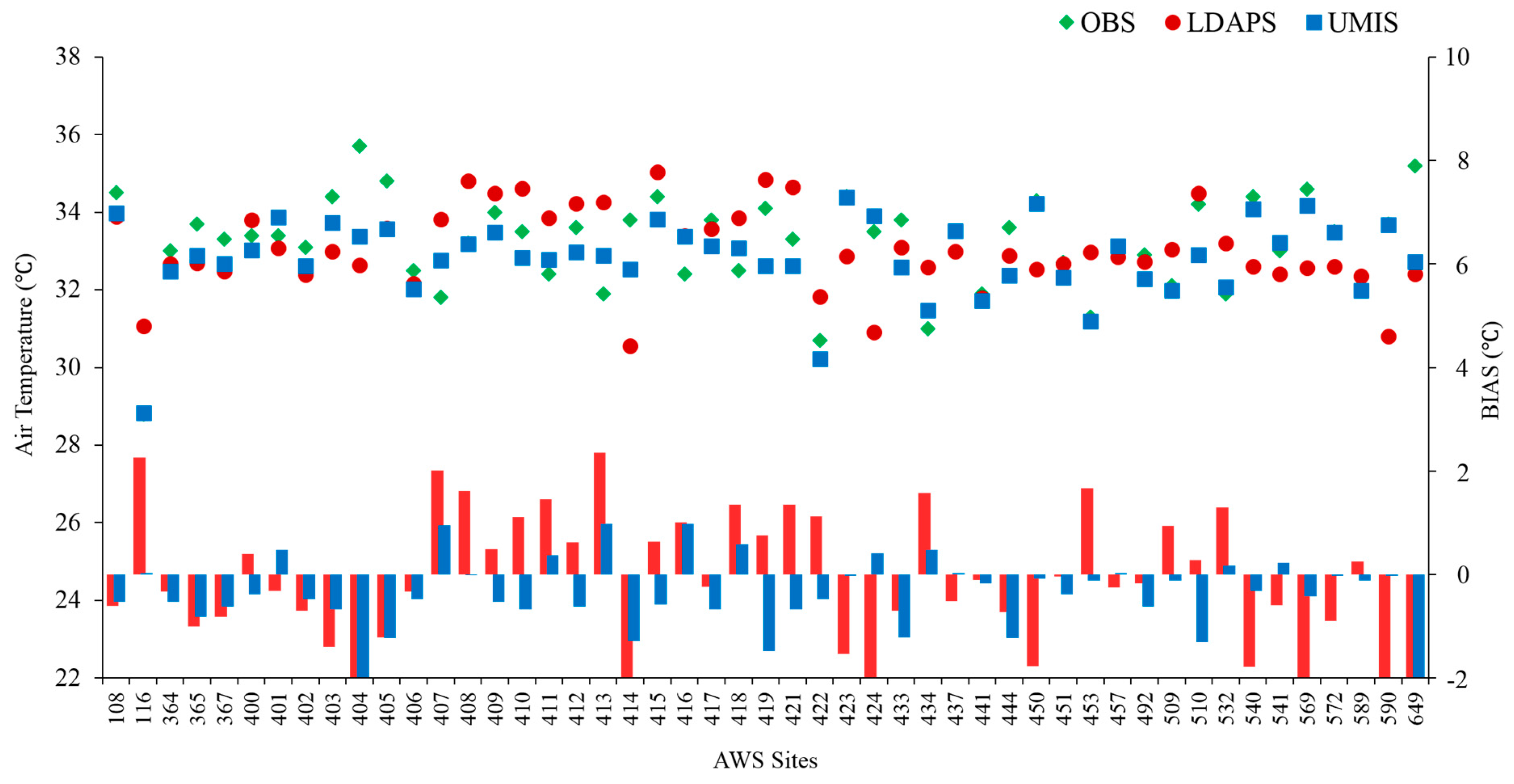
3.2. Accuracy Evaluation of Maximum Temperature during a Heatwave Episode

We performed an accuracy evaluation of the UMIS temperature prediction on the basis of the analog days corresponding to the heatwave forecast day. First, observed temperature data were collected from 50 AWSs and compared with temperature data predicted using LDAPS and UMIS (August 4, 2017, 06:00 UTC; Figure 8). Notable spatial differences were observed in the observed daytime temperatures from one AWS to another. Yi et al. [31] noted that such spatial differences are ascribable to the different shapes and sizes of urban surface components. In Figure 8, UMIS shows greater spatial differences than LDAPS in the predicted temperature when checked against the corresponding AWS observations. This is due to the susceptibility of the UMIS results to the influence of microclimatic thermal effect arising from the surface characteristics and structure of the area covered by each AWS. Accordingly, UMIS prediction results show a similar distribution profile to that of the AWS observations compared with the LDAPS prediction results that show less variations in temperature distribution according to land use. In a comparison using standard deviations as well, UMIS had less over- or under-estimation than LDAPS with lower standard deviations. As a result of accuracy validation, the RMSE and CC of LDAPS were calculated at 1.43 °C and 0.23, and those of UMIS were 0.8 °C and 0.81, demonstrating that UMIS contributes to improving LDAPS prediction outcomes.

Then, the predicted temperature distribution profiles in the Seoul Metropolitan Area and Gangnam district were compared between LDAPS and UMIS to evaluate the accuracy improvement through spatial distribution (Figure 9). LDAPS showed clearly different temperature distributions between the city core and its periphery, with the former 2–3 °C higher (34–35 °C vs. 31–32 °C). In addition to this spatial distribution profile of LDAPS-predicted temperatures, UMIS was exposed to microclimatic thermal effects arising from urban surface characteristics and structure. Accordingly, this microclimatic thermal effect was reflected in the LDAPS-predicted temperatures by an empirical equation based on the training data made up of observed temperature data and urban surface characteristics parameters. As a result, areas with high building footprint density and impervious surfaces were found to be more susceptible to temperature rise in the surrounding area, and vegetated areas such as parks and street trees in the city core showed temperatures lower than the surrounding core area.

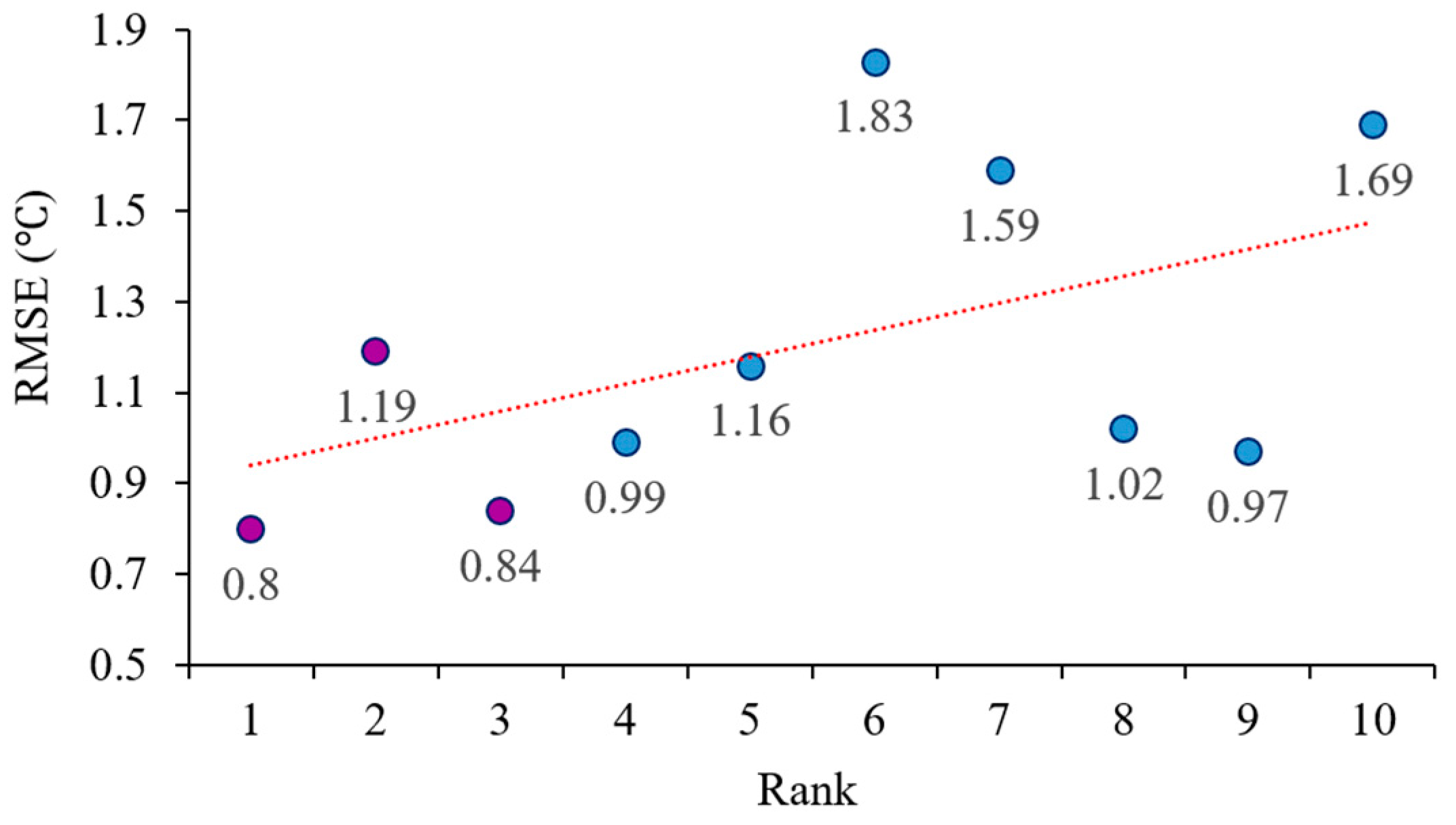
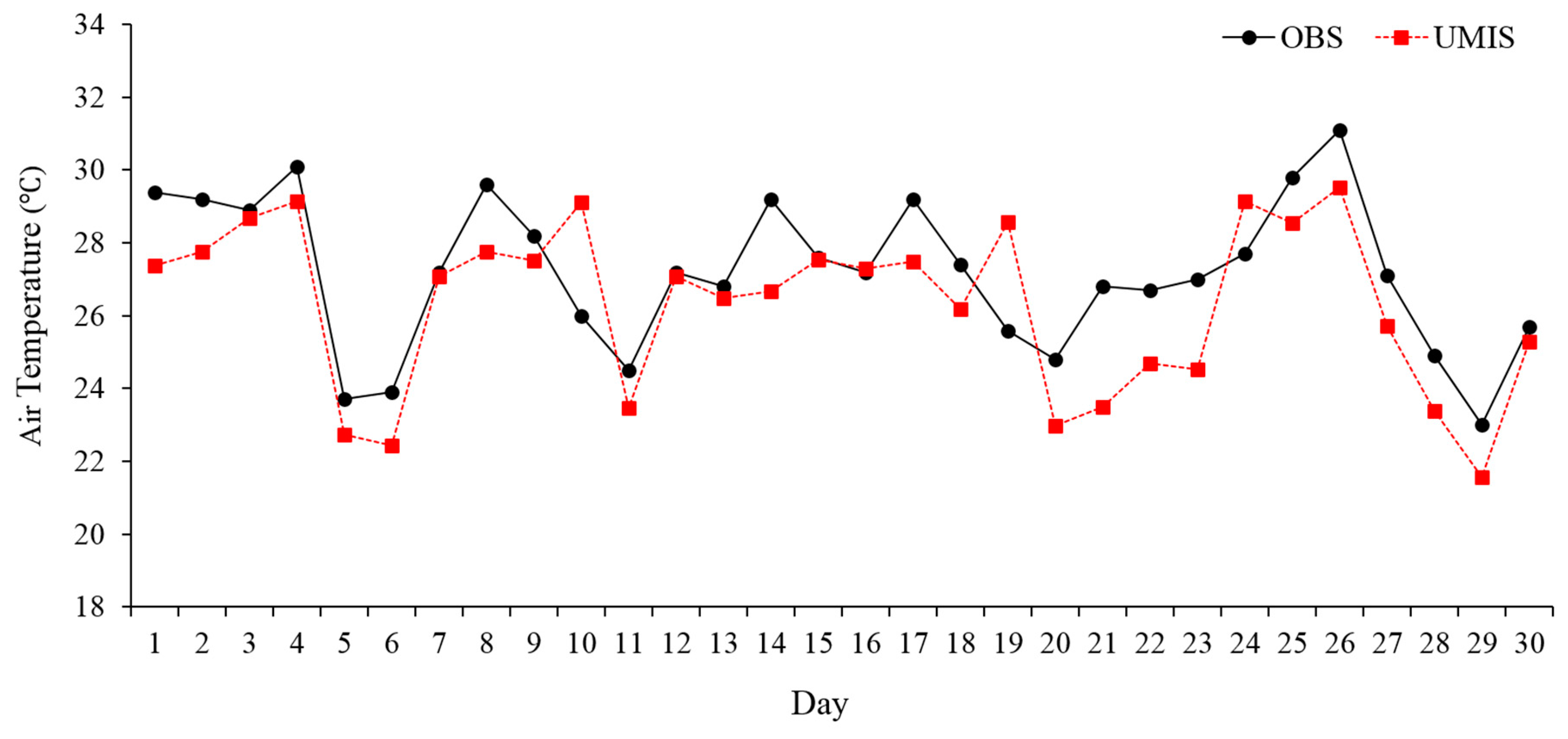
3.3. Accuracy Evaluation of Minimum Temperature during a Tropical Night

We also performed an accuracy evaluation of the UMIS temperature prediction results for August 4, 2017 (21:00 UTC), the results of which included the highest daily minimum temperature among the tropical night episodes. Observed temperature data were collected from 50 AWSs and compared with the temperature data predicted by LDAPS and UMIS (Figure 10). AWS-dependent spatial deviations were more conspicuous at dawn than during the daytime. Yi et al. [31] noted that such spatial differences are attributable to different shapes and sizes of urban surface components. Earlier studies have attributed such temperature deviations to temperature decline through cold air generation due to higher albedo in vegetated surfaces and the increase in sensible heat release into the atmosphere from building surfaces during the night, depending on the surface area ratio [44,45]. In the case of LDAPS, AWS-dependent temperature variations appeared at dawn to a greater extent than during the daytime, owing to a higher thermal effect of land use. Likewise, UMIS showed a greater thermal effect due to urban surface characteristics, demonstrating a temperature distribution profile closer to that of the observed temperature distribution. In a comparison of the deviation between LDAPS and UMIS, LDAPS did not reflect the effect of the heat released during the night according to the urban surface characteristics for reasons of resolution, resulting in underestimation in most areas, and UMIS exhibited smaller deviations in most areas. As a result of the accuracy validation, the RMSE and CC of LDAPS were calculated to be 1.29 °C and 0.66, respectively, and those of UMIS were calculated to be 0.51 °C and 0.95, respectively, demonstrating that UMIS also contributes to improving LDAPS prediction outcomes during the dawn hours.

The predicted temperature distribution profiles for the Seoul metropolitan area and Gangnam district were compared between LDAPS and UMIS (Figure 11). LDAPS showed clearly different spatial temperature distributions between the city core and surrounding mountainous area, with the former higher than the latter by 2–3 °C (27–29 °C vs. 23–25 °C). In the case of UMIS, temperature deviations were more conspicuous in the urban-scale city core, owing to the heat island effect, which persists for long periods of time because of the high building footprint and heat released from human-made structures. In contrast, vegetated areas in surrounding mountainous areas undergo a large temperature drop during the night. These results suggest that prediction accuracy during the night and dawn hours can be further improved by UMIS, with the effects of temperature decline at night and dawn more than offsetting the effect of temperature rise during the daytime as a result of urban surface characteristics.

3.4. Accuracy Evaluation Associated with Precipitation Episodes and Seasonal Fluctuations

We also evaluated the temperature prediction accuracy in relation to precipitation episodes and seasonal fluctuations. In a comparable study by Yi et al. [24], temperature overestimation occurred when an abrupt precipitation episode was simulated.

From among the precipitation days during the summer months, August 15, 2017 was selected as the forecast day. The day was characterized by a high daily average degree of cloud cover of 9.9 (on a scale of 0 to 10) and a sharp decline in the daily maximum temperature of approximately 5.7 °C from the level of the previous day. We graphically compared the hourly observed temperature on the precipitation day at the Seoul weather station (AWS #108) with the corresponding precipitation data and UMIS-predicted temperatures (Figure 12).

The temperature was observed to decline gradually in the hours before precipitation began, and the UMIS outputs also decreased to a similar extent. In the time segment during which precipitation occurred, the UMIS results exhibited a temperature distribution similar to the AWS observations. While slightly overestimated outputs appeared during the daytime, the overall prediction accuracy improved in comparison to that obtained with the sliding window technique.

We then graphically compared the daily maximum temperatures observed at the Seoul weather station (AWS #108) and the UMIS-predicted temperatures to evaluate the UMIS prediction accuracy with regards to seasonal fluctuations (Figure 13). The UMIS predictions of daytime temperatures in September exhibited stable performance, without any significant underestimation (the temperature was predicted to be lower than the observed value) because of the low frequency of extreme heat, as in July and August, or overestimation (the temperature was predicted to be higher than the observed value), as in the sliding window technique. Thus, the MOS-Analog technique was found to be able to overcome the limitation of the sliding window technique, which cannot take into account precipitation and seasonal fluctuations that deviate from the latest temperature trends. These results demonstrate the potential for UMIS to produce stable outputs.

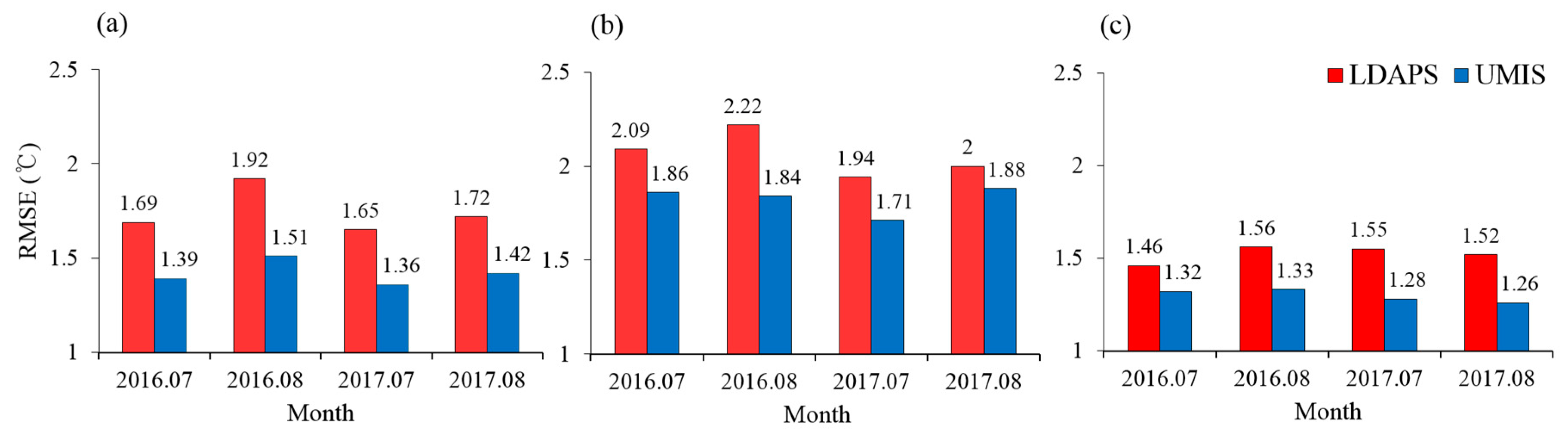
3.5. Prediction Accuracy of Daily Maximum and Minimum Temperatures in Summer

We performed an accuracy validation of statistical downscaling using the MOS-Analog technique with regard to the daily maximum and minimum temperatures during the summer months (July and August 2016 and 2017, 00:00–23:00 every hour).

First, the hourly LDAPS- and UMIS-predicted temperatures were compared to the real-time AWS observations. Next, the respective mean monthly values of RMSE and CC were calculated (Figure 14a): 1.64 °C and 0.4, respectively, for LDAPS and 1.22 °C and 0.7, respectively, for UMIS. The application of the MOS-Analog technique resulted in a 25% decrease in RMSE and a 0.3 increase in CC. With the bias correction effect achieved through analog daytime temperature observations and the microclimatic thermal effect due to time-dependent urban surface characteristics being reflected in the LDAPS prediction results, the UMIS prediction accuracy was found to improve every hour.

Next, we compared the temperature prediction results for the daily maximum temperature time slot with the real-time AWS observations and obtained their monthly averages (Figure 14b). The RMSE and CC for LDAPS were calculated as 2 °C and 0.4, respectively, and those for UMIS were 1.65 °C and 0.7, respectively. The overall averages throughout the observation period resulted in a 20% decrease in RMSE and a 0.3 increase in CC.

Last, we compared the temperature prediction results for the daily minimum temperature time slot with the real-time AWS observations and obtained their monthly average (Figure 14c). The RMSE and CC of LDAPS were calculated to be 1.52 °C and 0.46, respectively, and those of UMIS were 1.30 °C and 0.73, respectively. The overall average throughout the observation period resulted in a 15% decrease in RMSE and a 0.3 increase in CC.

The temperature rise effect due to sensible heat release from the thermal energy stored during the day in the city’s core and the temperature drop effect due to the cold air generated during the night in vegetated areas may be explained by the results of a previous study that describe the large contribution of the quantitative distribution of observed air temperatures at the ground surface [31]. Therefore, as these two effects based on quantitative distributions of temperatures at the ground surface are reflected in the UMIS prediction data, the UMIS prediction accuracy for the daily maximum and minimum temperatures can be said to have improved.

4. Conclusions

In this study, we performed statistical downscaling of air temperature prediction results with 1.5 km resolution (UM-LDAPS) for the Seoul metropolitan area to 25 m resolution, using the MOS-Analog technique described in this paper and carried out bias correction. CAS-computed urban surface parameters and AWS observations were used as training data, and SVM machine learning was used as an empirical computational model. Using temperature data predicted by the MOS-Analog-based UMIS, the prediction accuracy with regard to analog days, heat days, daily maximum and minimum temperatures, inclusion of precipitation days, seasonal features, and summer temperatures (hourly, daily maximum, and daily minimum) was improved. Through these predictions and their evaluations, we assessed the suitability of the statistical downscaling method using the MOS-Analog technique for microclimatic research.

With the bias correction effect through analog day temperature observations and microclimatic thermal effect due to time-dependent urban surface characteristics reflected in the LDAPS prediction results, the UMIS prediction accuracy was found to improve every hour. With the temperature rise effect due to the sensible heat released from city core land use and building structures, the temperature rise effect due to the release of sensible heat stored in the city core during the day and the temperature drop effect in vegetated areas due to cold air generation during the night being reflected in the LDAPS prediction results, the UMIS prediction accuracy for both daytime and nighttime improved. Furthermore, the UMIS results for precipitation periods were found to show temperature distribution profiles similar to those of observed temperatures, and stable performance was also maintained in cases reflecting seasonal features. It was thus verified that UMIS prediction accuracy improved in all time slots, precipitation days, and episodes reflecting seasonal features, which confirms that the MOS-Analog-based statistical downscaling technique described in this paper can be applied to urban-scale meteorology research.

The statistical downscaling approaches employed to date in other studies have mostly been associated with global or regional-scale climate models (GCM or RCM). However, to provide detailed explanations of urban-scale weather phenomena triggered by complex urban spatial structures, numerical weather prediction models should also have sufficiently high resolutions. To meet this need, we performed a statistical downscaling process on the LDAPS with a local-scale resolution (1.5 km grid). Given its short operation history (4 years since the last computation), there are not many printed LDAPS data values available. Another disadvantage is its limited ability to compute analog days for want of available data, given that it does not have recourse to weather pattern simulations, because of the nature of analog analysis. However, hourly temperature, which is a variable of interest, exhibits regular hourly, daily, and seasonal patterns, and the temperature distribution profiles of time slots with the same cycle are very similar. Despite the limited quantity of available data, MOS-Analog-based statistical downscaling was carried out in this study with 3 years of LDAPS datasets. As a result, the applicability of the statistical downscaling technique employed in this study has been verified. The number of analog day candidates increases as the number of LDAPS data increases, which contributes to enhancing prediction accuracy through output correction with respect to analog days with near-true values.

The results of this study suggest that the statistical downscaling approach proposed in this study for microclimatic information extraction can be applied to solving problems related to urban-scale meteorology, such as urban planning, as well as its potential applicability to other metropolitan areas in need of microclimatic research.

References

1. Themeßl, M.J.; Gobiet, A.; Leuprecht, A. Empirical-statistical downscaling and error correction of daily precipitation from regional climate models. Int. J. Climatol. 2011, 31, 1530–1544. [Google Scholar] [CrossRef]
2. Lemonsu, A.; Viguie, V.; Daniel, M.; Masson, V. Vulnerability to heat waves: Impact of urban expansion scenarios on urban heat island and heat stress in Paris (France). Urban Clim. 2015, 14, 586–605. [Google Scholar] [CrossRef]
3. Metzger, K.B.; Ito, K.; Matte, T.D. Summer heat and mortality in New York City: How hot is too hot? Environ. Health Perspect. 2009, 118, 80–86. [Google Scholar] [CrossRef] [PubMed]
4. Baklanov, A.; Grimmond, C.S.B.; Carlson, D.; Terblanche, D.; Tang, X.; Bouchet, V.; Lee, B.; Langendijk, G.; Kolli, R.K.; Hovsepyan, A. From urban meteorology, climate and environment research to integrated city services. Urban Clim. 2018, 23, 330–341. [Google Scholar] [CrossRef]
5. Herdt, A.J. A multi-index investigation of the spatiotemporal relationships between heat and EMS calls during the 2015 pan American games in Toronto, Canada, 2017. MA Thesis, Texas Tech University, Lubbock, TX, USA, August 2017. [Google Scholar]
6. Tan, J.; Yang, L.; Grimmond, C.S.B.; Shi, J.; Gu, W.; Chang, Y.; Hu, P.; Sun, J.; Ao, X.; Han, Z. Urban integrated meteorological observations: Practice and experience in Shanghai, China. Bull. Am. Meteorol. Soc. 2015, 96, 85–102. [Google Scholar] [CrossRef]
7. Yi, C.; Kwon, H.G.; Kim, K.R.; An, S.M.; Choi, Y.J.; Scherer, D. Climate information application for improved planning and management of cities. In Proceedings of the ICUC Annual Meeting, Toulouse, France, 20–24 July 2015. [Google Scholar]
8. Fowler, H.J.; Blenkinsop, S.; Tebaldi, C. Linking climate change modelling to impacts studies: Recent advances in downscaling techniques for hydrological modelling. Int. J. Climatol. 2007, 27, 1547–1578. [Google Scholar] [CrossRef]
9. Herrera, S.; Fita, L.; Fernández, J.; Gutiérrez, J.M. Evaluation of the mean and extreme precipitation regimes from the ENSEMBLES regional climate multimodel simulations over Spain. J. Geophys. Res. Atmos. 2010, 115. [Google Scholar] [CrossRef] [Green Version]
10. Seguí, P.Q.; Ribes, A.; Martin, E.; Habets, F.; Boé, J. Comparison of three downscaling methods in simulating the impact of climate change on the hydrology of mediterranean basins. J. Hydrol. 2010, 383, 111–124. [Google Scholar] [CrossRef]
11. Fowler, H.J.; Ekström, M. Multi-model ensemble estimates of climate change impacts on UK seasonal precipitation extremes. Int. J. Climatol. 2009, 29, 385–416. [Google Scholar] [CrossRef]
12. Yi, C.; An, S.M.; Kim, K.; Kwon, H.; Min, J.-S. Surface micro-climate analysis based on urban morphological characteristics: Temperature deviation estimation and evaluation. Atmos. Korea 2016, 26, 445–459. [Google Scholar] [CrossRef]
13. Wilks, D.S.; Wilby, R.L. The weather generation game: A review of stochastic weather models. Prog. Phys. Geogr. 1999, 23, 329–357. [Google Scholar] [CrossRef]
14. Caillouet, L.; Vidal, J.-P.; Sauquet, E.; Graff, B. Probabilistic precipitation and temperature downscaling of the twentieth century reanalysis over France. Clim. Past 2016, 12, 635–662. [Google Scholar] [CrossRef]
15. Oh, J.-H.; Kim, T.; Kim, M.-K.; Lee, S.-H.; Min, S.-K.; Kwon, W.-T. Regional climate simulation for Korea using dynamic downscaling and statistical adjustment. J. Meteorol. Soc. Jpn. Ser. II 2004, 82, 1629–1643. [Google Scholar] [CrossRef]
16. Kim, K.B.; Kwon, H.-H.; Han, D. Bias correction methods for regional climate model simulations considering the distributional parametric uncertainty underlying the observations. J. Hydrol. 2015, 530, 568–579. [Google Scholar] [CrossRef] [Green Version]
17. Maraun, D.; Wetterhall, F.; Ireson, A.M.; Chandler, R.E.; Kendon, E.J.; Widmann, M.; Brienen, S.; Rust, H.W.; Sauter, T.; Themeßl, M.; et al. Precipitation downscaling under climate change: Recent developments to bridge the gap between dynamical models and the end user. Rev. Geophys. 2010, 48. [Google Scholar] [CrossRef]
18. Dallavalle, J.P. A perspective on the use of model output statistics in objective weather forecasting. In Proceedings of the 15th Conference on Weather Analysis and Forecasting, Norfolk, VA, USA, 19–23 August 1996; Volume 15, pp. 479–482. [Google Scholar]
19. Fuentes, U.; Heimann, D. An improved statistical-dynamical downscaling scheme and its application to the alpine precipitation climatology. Theor. Appl. Climatol. 2000, 65, 119–135. [Google Scholar] [CrossRef]
20. Imbert, A.; Benestad, R.E. An improvement of analog model strategy for more reliable local climate change scenarios. Theor. Appl. Climatol. 2005, 82, 245–255. [Google Scholar] [CrossRef]
21. Liaw, A.; Wiener, M. Classification and regression by randomforest. R News 2002, 2, 18–22. [Google Scholar]
22. Keramitsoglou, I.; Kiranoudis, C.T.; Weng, Q. Downscaling geostationary land surface temperature imagery for urban analysis. IEEE Geosci. Remote Sens. Lett. 2013, 10, 1253–1257. [Google Scholar] [CrossRef]
23. Yoo, C.; Im, J.; Park, S.; Quackenbush, L.J. Estimation of daily maximum and minimum air temperatures in urban landscapes using MODIS time series satellite data. ISPRS J. Photogramm. Remote Sens. 2018, 137, 149–162. [Google Scholar] [CrossRef]
24. Yi, C.; Shin, Y.; Roh, J.W. Development of an urban high-resolution air temperature forecast system for local weather information services based on statistical downscaling. Atmosphere 2018, 9, 164. [Google Scholar] [CrossRef]
25. Turco, M.; Llasat, M.C.; Herrera, S.; Gutiérrez, J.M. Bias correction and downscaling of future RCM precipitation projections using a MOS-analog technique. J. Geophys. Res. 2017, 122, 2631–2648. [Google Scholar] [CrossRef]
26. Stewart, I.D.; Oke, T.R. Local climate zones for urban temperature studies. Bull. Am. Meteorol. Soc. 2012, 93, 1879–1900. [Google Scholar] [CrossRef]
27. Korea Meteorological Administration. Numerical Data Application Manual; KMA: Seoul, Korea, 2011; pp. 13–17.
28. Kim, K.R.; Yi, C.; Lee, J.-S.; Meier, F.; Jänicke, B.; Fehrenbach, U.; Scherer, D. BioCAS: Biometeorological climate impact assessment system for building-scale impact assessment of heat-stress related mortality. DIE ERDE J. Geogr. Soc. Berl. 2014, 145, 62–79. [Google Scholar]
29. Yi, C.Y.; Choi, Y.-J.; Eum, J.-H.; Kim, G.H.; Rang, K.; Kim, D.S.; Fehrenbach, U. Development of Climate Analysis Software for Urban and Environmental Planning of Seoul; Berichte des Meteorologischen Instituts der Albert-Ludwigs-Universität Freiburg: Freiburg, Germany, 2010; p. 455. [Google Scholar]
30. Yi, C.; Kim, K.R.; An, S.M.; Choi, Y.-J.; Holtmann, A.; Jänicke, B.; Fehrenbach, U.; Scherer, D. Estimating spatial patterns of air temperature at building-resolving spatial resolution in Seoul, Korea. Int. J. Climatol. 2016, 36, 533–549. [Google Scholar] [CrossRef]
31. Yi, C.-Y.; Kim, K.-R.; An, S.-M.; Choi, Y.-J. Impact of the local surface characteristics and the distance from the center of heat island to suburban areas on the night temperature distribution over the Seoul metropolitan area. J. Korean Assoc. Geogr. Inf. Stud. 2014, 17, 35–49. [Google Scholar] [CrossRef]
32. Wilks, D.S. Statistical methods in the atmospheric sciences; Academic Press: Cambridge, MA, USA, 2011; Volume 100. [Google Scholar]
33. Déqué, M. Frequency of precipitation and temperature extremes over France in an anthropogenic scenario: Model results and statistical correction according to observed values. Glob. Planet. Chang. 2007, 57, 16–26. [Google Scholar] [CrossRef]
34. Widmann, M.; Bretherton, C.S.; Salathé, E.P., Jr. Statistical precipitation downscaling over the Northwestern United States using numerically simulated precipitation as a predictor. J. Clim. 2003, 16, 799–816. [Google Scholar] [CrossRef]
35. Lorenz, E.N. Deterministic nonperiodic flow. J. Atmos. Sci. 1963, 20, 130–141. [Google Scholar] [CrossRef]
36. Lorenz, E.N. Atmospheric predictability as revealed by naturally occurring analogues. J. Atmos. Sci. 1969, 26, 636–646. [Google Scholar] [CrossRef]
37. Zorita, E.; Hughes, J.P.; Lettemaier, D.P.; von Storch, H. Stochastic characterization of regional circulation patterns for climate model diagnosis and estimation of local precipitation. J. Clim. 1995, 8, 1023–1042. [Google Scholar] [CrossRef]
38. Matulla, C.; Zhang, X.; Wang, X.L.; Wang, J.; Zorita, E.; Wagner, S.; Von Storch, H. Influence of similarity measures on the performance of the analog method for downscaling daily precipitation. Clim. Dyn. 2008, 30, 133–144. [Google Scholar] [CrossRef]
39. Gutiérrez, J.M.; San-Martín, D.; Brands, S.; Manzanas, R.; Herrera, S. Reassessing statistical downscaling techniques for their robust application under climate change conditions. J. Clim. 2013, 26, 171–188. [Google Scholar] [CrossRef]
40. Radanovics, S.; Vidal, J.-P.; Sauquet, E.; Daoud, A.B.; Bontron, G. Optimising predictor domains for spatially coherent precipitation downscaling. Hydrol. Earth Syst. Sci. 2013, 17, 4189–4208. [Google Scholar] [CrossRef] [Green Version]
41. Turco, M.; Quintana-Seguí, P.; Llasat, M.C.; Herrera, S.; Gutiérrez, J.M. Testing MOS precipitation downscaling for ensembles regional climate models over Spain. J. Geophys. Res. Atmos. 2011, 116, 1–14. [Google Scholar] [CrossRef]
42. Cherkassky, V.; Ma, Y. Practical selection of SVM parameters and noise estimation for SVM regression. Neural Netw. 2004, 17, 113–126. [Google Scholar] [CrossRef] [Green Version]
43. Karatzoglou, A.; Smola, A.; Hornik, K.; Maniscalco, M.A.; Teo, C.H. Package Kernlab-CRAN. Available online: https://cran.r-project.org/web/packages/kernlab/index.html (accessed on 25 July 2019).
44. Christen, A.; Vogt, R. Energy and radiation balance of a central european city. Int. J. Climatol. 2004, 24, 1395–1421. [Google Scholar] [CrossRef]
45. Yi, C.-Y.; An, S.-M.; Kim, K.-R.; Choi, Y.-J.; Scherer, D. Improvement of air temperature analysis by precise spatial data on a local-scale-a case study of Eunpyeong new town in Seoul. J. Korean Assoc. Geogr. Inf. Stud. 2012, 15, 144–158. [Google Scholar] [CrossRef]
Figure 1. Topographic and land cover characteristics of Seoul. (a) Aerial photograph (yellow line denotes the administrative boundary of Seoul); (b) local climate zone (LCZ) types of land surfaces with building footprints; (c) shaded relief map; and (d) street networks (white) and automated weather stations (AWSs; yellow dots).
Atmosphere 10 00427 g001
Figure 2. Number of patients with heat-related illness and number of heat days (those with daily maximum temperatures >33 °C) in Seoul (sources: National Health Insurance Service and Korea Meteorological Administration).
Atmosphere 10 00427 g002
Figure 3. Model computation area. (a) South Korea; (b) air temperature forecast for the Seoul metropolitan area 1.5 m above the ground.
Atmosphere 10 00427 g003
Figure 4. Built-up and impervious surface fractions in areas within a 100-m radius of individual AWSs in the Seoul Metropolitan Area (n = 50). (a) Fractional coverage of built-up surfaces; (b) fractional coverage of impervious surfaces.
Atmosphere 10 00427 g004
Figure 5. Rank according to Euclidean distance computed from prediction parameters (x-axis). Root mean square error (RMSE) computations of case dates depending on the Euclidean distance (y-axis). (a) Overall case dates (blue), filtering conditions applied to each parameter; (b) temperature (orange); (c) wind (red); and (d) relative humidity (green).
Atmosphere 10 00427 g005
Figure 6. Rank according to Euclidean distance computed from prediction parameters (x axis). Root mean square error computations of analog days (forecast day: August 4, 2017, 06:00 UTC).
Atmosphere 10 00427 g006
Figure 7. 1.5-m temperature distribution from LDAPS across South Korea, including the study region: (a) The forecast day (4 August 2017, 06:00 Coordinated Universal Time (UTC)); (b) first analog day (4 August 2017, 05:00 UTC); (c) second analog day (10 August 2016, 06:00 UTC); and (d) third analog day (18 August 2016, 04:00 UTC). CORR = correlation coefficient.
Atmosphere 10 00427 g007
Figure 8. Evaluation of the temperature at the time of daily maximum temperature per automated weather station (AWS; forecast day: 04 August 2017 06:00 UTC). OBS, observed data; LDAPS, Local Data Assimilation and Prediction System; UMIS, Urban Meteorological Information System.
Atmosphere 10 00427 g008
Figure 9. Spatial accuracy evaluation for the heatwave period (forecast day: August 4, 2017, 06:00 UTC). (a) Map of Seoul; (b) local data assimilation and prediction system (LDAPS) temperatures across Seoul; (c) urban meteorological information system (UMIS) temperatures across Seoul; (d) map of the Gangnam district; (e) LDAPS temperatures across the Gangnam district; (f) UMIS temperatures across the Gangnam district.
Atmosphere 10 00427 g009
Figure 10. Validation of the temperature at the time of the daily minimum temperature for each automated weather station (AWS; forecast day: 04 August 2017 21:00 UTC). OBS, observed data; LDAPS, Local Data Assimilation and Prediction System; UMIS, Urban Meteorological Information System.
Atmosphere 10 00427 g010
Figure 11. Spatial accuracy evaluation for a tropical night (forecast day: August 4, 2017, 21:00 UTC). (a) Map of Seoul; (b) local data Assimilation and prediction system (LDAPS) temperatures across Seoul; (c) urban meteorological information system (UMIS) temperatures across Seoul; (d) map of the Gangnam district; (e) LDAPS temperatures across the Gangnam district; (f) UMIS temperatures across the Gangnam district.
Atmosphere 10 00427 g011
Figure 12. Accuracy evaluation for unforeseen events and seasonal fluctuations. Meteorological variable value for the Seoul weather station (AWS #108): OBS_PREC, observed precipitation; OBS, observed air temperature; UMIS, Urban Meteorological Information System.
Atmosphere 10 00427 g012
Figure 13. Accuracy evaluation for unforeseen events and seasonal fluctuations. Daily maximum temperature at the Seoul weather station (AWS #108): OBS, observed data; LDAPS, Local Data Assimilation and Prediction System; UMIS, Urban Meteorological Information System.
Atmosphere 10 00427 g013
Figure 14. Assessment of the downscaled temperature from post-processing. (a) All hourly temperatures; (b) daily maximum temperature; (c) daily minimum temperature. LDAPS, Local Data Assimilation and Prediction System; UMIS, Urban Meteorological Information System.
Atmosphere 10 00427 g014