Comparing Statistical and Semi-Distributed Rainfall–Runoff Models for a Large Subtropical Watershed: A Case Study of Jiulong River Catchment, China

Abstract

In this contribution, the authors present their preliminary investigations into modeling the rainfall–runoff generation relation in a large subtropical catchment (Jiulong River catchment) on the southeast coast of China. Previous studies have mostly focused on modeling the streamflow and water quality of its small rural subcatchments. However, daily runoff on the scale of the whole catchment has not been modeled before, and hourly runoff data are desirable for some oceanographic applications. Three methods are proposed for modeling streamflow using rainfall outputted by the Weather Research Forecast (WRF) model, calculated potential evaporation (PET), and land cover type: (i) a ridge regression model; (ii) NPRED-KNN: a nonparametric k-nearest neighbor model (KNN) employing a parameter selection method (NPRED) based on partial information coefficient; (iii) the Hydrological Simulation Program-Fortran (HSPF) model with an hourly time step. Results show that the NPRED-KNN approach is the most unsuitable method of those tested. The HSPF model was manually calibrated, and ridge regression performs no worse than HSPF based on daily verification, whilst HSPF can produce realist daily flow time series, of which ridge regression is incapable. The HSPF model seems less prone to systematic underprediction when replicating monthly-annual water balance, and it successfully replicates the baseflow index (the flow intensity) of the Jiulong River catchment system.

1. Introduction and Motivation

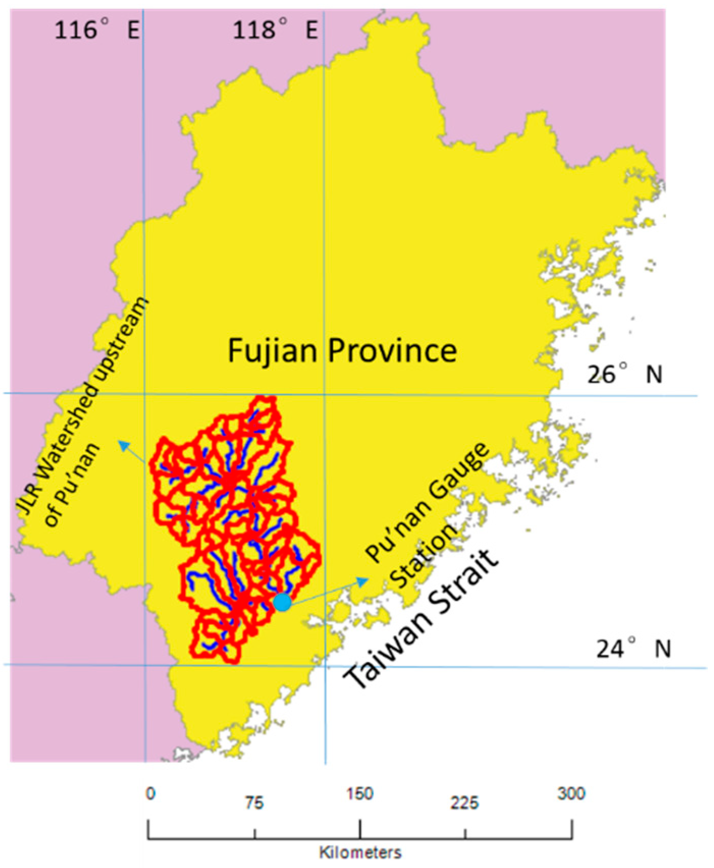
The Jiulong River (JLR) runs 258 km through a subtropical catchment situated at 24.2–25.8° N, 117–118° E in Fujian Province, on the southeast coast of China (Figure 1), covering an area of 14,700 km². The JLR consists of two major branches: North Stream (Bei’Xi) and West Stream (Xi’Xi) (Figure 3). The annual average runoff of the catchment is 1.2 × 10¹⁰ m³, with over two-thirds of the total runoff contributed by the North Stream. The catchment shows significant intra-annual unevenness in precipitation, as approximately 70% of the total runoff occurs during April–September due to typhoon and tropical storm events. The catchment is largely rural, where over 60% of the total area is woodlands [1].

Figure 1. Location of the Jiulong River (JLR) watershed (the portion upstream of the Pu’nan gauge station); the blue and red lines present the river and ridge, respectively.

Previous research on JLR hydrology has mainly focused on the water quality [2] and land use impact [1], and models that compute daily or monthly total runoff suffice for these purposes (e.g., AnnAGNPS (Annualized Agricultural Non-Point Source) used in [2]). However, for other purposes, runoff with finer temporal resolution is more preferable. Examples include those where the timing of the freshwater runoff is important, such as when providing boundary conditions for estuarine dynamic models for the study of estuarine stratification [3,4] and determining the interaction between fluvial flood and storm surges [5]. Other applications for which hourly runoff input is desirable include harmonic analyses of estuarine tides influenced by river runoff [6,7]. The main intention of this work is to investigate how useful a rainfall forecast of limited accuracy (but readily available to ocean modelers) obtained using operational Weather Research Forecast (WRF) models are for modeling the (hourly) streamflow of the JLR catchment. An example of using an ensemble WRF rainfall forecast for TOPMODEL (TOPography-based Hydrological MODEL) can be found in [8]. In our work, as no ensemble or probabilistic technique is used for improving WRF output quality, the relatively large deviation of model outputs from observations can be a critical source of errors in the streamflow hindcast; so, this issue will be briefly and qualitatively discussed.

Here, we attempt to compare three approaches to modeling the rainfall–runoff generation in the JLR catchment: (1) ridge regression, (2) k-nearest neighbor regression employing precipitation output of the Weather Research and Forecast model (WRF) and the computed potential evapotranspiration, and (3) the Hydrological Simulation Program-Fortran (HSPF) model with hourly output. The application of the first approach was inspired by the preliminary multivariate linear regression (MLR) analysis, and the application of MLR to streamflow forecasting can be found in [9]. The second approach was proposed by Lall and Sharma [10] and has been widely adopted as a nonparametric method for streamflow prediction and disaggregation [11,12,13] (the NPRED-KNN (k-nearest neighbor) package can be downloaded from http://www.hydrology.unsw.edu.au/download/software/npred). HSPF has also been widely adopted for hydrological modeling of large catchments, not only in the United States [14,15,16] where the toolkit was developed but in other countries as well (e.g., China: [17,18,19,20]). It is free, supports hourly output, and has a semi-distributed, physically based routing component (with channel geometries inferred from topography data), making it applicable for modeling complex, large catchments. Although the models can only be compared with the daily measurements taken at the Pu’nan gauge station, all these methods are easily extensible to hourly outputs.

MLR has been previously implemented for some small and (or) semi-arid watersheds smaller than 1000 km² ([21,22]). Here, as the regression technique was applied to a larger, humid, and heavy watershed (thus having more diverse and complex features than the semi-arid ones), more predictors were required, introducing multicollinearity to the problem. To deal with multicollinearity, ridge regression was adopted.

The NPRED-KNN method adopted in this work is intended to be an example of a nonparametric soft computing strategy. Other alternatives include combining machine learning techniques (e.g., artificial neural network (ANN), $\mathsf{ϵ}-$ support vector machine with a nonlinear kernel) with some time series decomposition/spectral analysis methods (e.g., singular spectrum, empirical mode decomposition) ([9,23]). Given the scarcity of data and previous study of JLR streamflow simulation, as well as the fact that we are focusing on the feasibility of using the less accurate but readily available rainfall simulation for runoff estimation, at this stage, we would like to keep things simple and rely more on some less sophisticated techniques (e.g., ridge regression, KNN). The majority of the paper deals with the methodology we adopted for modeling, followed by the presentation and comparison of model results. A brief discussion on the (1) computation of baseflow index using HSPF output and (2) the implication of the limited input rainfall accuracy is provided.

2. Data and Methodology

The data sources for building these models are listed in Table 1. The WRF model outputs (precipitation, 2 m temperature) are provided by the Fujian Marine Forecast Institute (http://www.fjmf.gov.cn). Note that there are some instances after the year 2015 where the WRF model failed to receive the background field information; hence, some values are missing (5% of the total data amount) from the WRF dataset. For these dates, the WRF rainfall and temperature data are replaced by the ERA-5 (European Centre for Medium-Range Weather Forecast Reanalysis-5, or ECMWF-Reanalysis5) hourly reanalysis [24]. ERA-5 is the state-of-the-art global weather reanalysis dataset developed by the European Centre for Medium-Range Weather Forecast, which assimilates a large number of historical observations into ECMWF’s model outputs through the 4D-VAR technique. The dataset has a temporal resolution of 1 h and a spatial resolution of 31 km [24,25], and, to our knowledge, it is probably the only global reanalysis dataset with a 1-hour temporal resolution. To accommodate the 0.2° resolution of the WRF model output, nearest-neighbor resampling was applied to the ERA-5 dataset. Also, in order to compare the model with observations, two meteorological stations’ data were selected: Zhangping (ZP; an upstream station near the source of the JLR) and Xiamen (XM; a station representative of the lower stream, coastal conditions). During 2010–2015, temperature measurements were usually taken at 6-hour intervals; from 2016 onwards, the temperature was measured every 3 h. For the whole period, the rainfall data were recorded every 6 h (total precipitation during the previous 6 h). The meteorological observations were downloaded from www.rp5.ru.

Table 1. Data sources.

Precipitation	WRF model output * + ERA5 Reanalysis **
2m Temperature	WRF model output + ERA5 Reanalysis	Inputs for hourly PET calculation
2m Dew Point Temperature	ERA5 – Reanalysis
Digital Elevation Model Data	SRTM 30 (Resolution: 90 m)
Flowrate at Pu’nan Gauge Station	Observation

* Hourly data, 0.2° grid; ** hourly data, 31 km resolution, nearest-neighbor—resampled to 0.2°.

The river runoff data used in this paper were measured at 08:00 every day at the Pu’nan gauge station in the lower course of the JLR, and the time range is 2010–2017. The runoff observation data were download from http://xxfb.hydroinfo.gov.cn/ssIndex.html.

The HSPF model, which is a semi-distributed hydrologic model, also requires topographic input for subcatchment and stream network delineation. The void-filled SRTM30 digital elevation model (DEM) [26], which is a combination of the data sourced from the Shuttle Radar Topography Mission and the previous U.S. Geological survey’s GTOPO30 dataset [27], was employed in the current study, as it is probably the publicly available global topography dataset with the highest resolution. The land cover information required by HSPF is based on MODIS’ MCD12 product [28] and Global Manmade Impervious Surface (GMIS) dataset v.1 ([29]; http://sedac.ciesin.columbia.edu/data/set/ulandsat-gmis-v1).

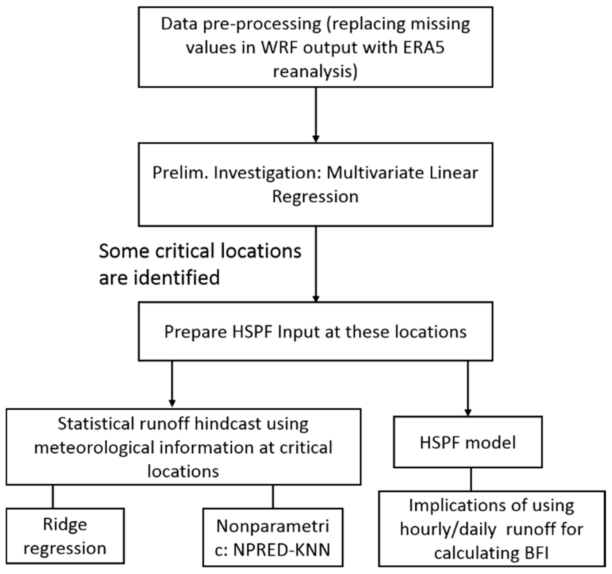
For all three models, only the discharge at the Pu’nan gauge station was computed. The North Stream (Bei’Xi) that drains into this station accounts for more than two-thirds of the total runoff generated in the catchment, so it is of greater significance to the estuarine and ecological processes in Xiamen Bay. A flowchart of our methodologies is presented below in Figure 2.

Figure 2. Flowchart of methodologies.

2.1. Data Preprocessing

2.1.1. Comparison with Observations

The WRF model tends to underestimate the temperature by 1.5 K and 2.35 K (after replacing missing values with ERA-5 reanalysis) for XM and ZP, respectively, and the root-mean-square error (RMSE) values are 2.75 K and 3.43 K.

Defining <0.1 mm (6-hour total) as no rainfall, Table 2 and Table 3 reveal that the WRF model significantly overestimates rainfall occurrence, and the model performance is slightly better at the inland ZP station (76% false positive vs. 82% false positive at XM).

Table 2. Rainfall occurrence (Xiamen (XM) and Zhangping (ZP)), Weather Research Forecast (WRF) outputs during 2010–2015. Obs/Mdl_dry means no rainfall in observation/model.

	Obs_dry	Obs_wet	Mdl_accuracy
Mdl_dry_XM	6396	1167	85%
Mdl_wet_XM	3133	684	18%
Mdl_dry_ZP	5386	1271	81%
Mdl_wet_ZP	3565	1110	24%

Table 3. Rainfall occurrence (XM and ZP), ERA-5 (European Centre for Medium-Range Weather Forecast Reanalysis-5).

	Obs_dry	Obs_wet	Mdl_accuracy
Mdl_dry_XM	5803	1027	85%
Mdl_wet_XM	4306	901	17%
Mdl_dry_ZP	5389	1262	81%
Mdl_wet_ZP	4075	1266	24%

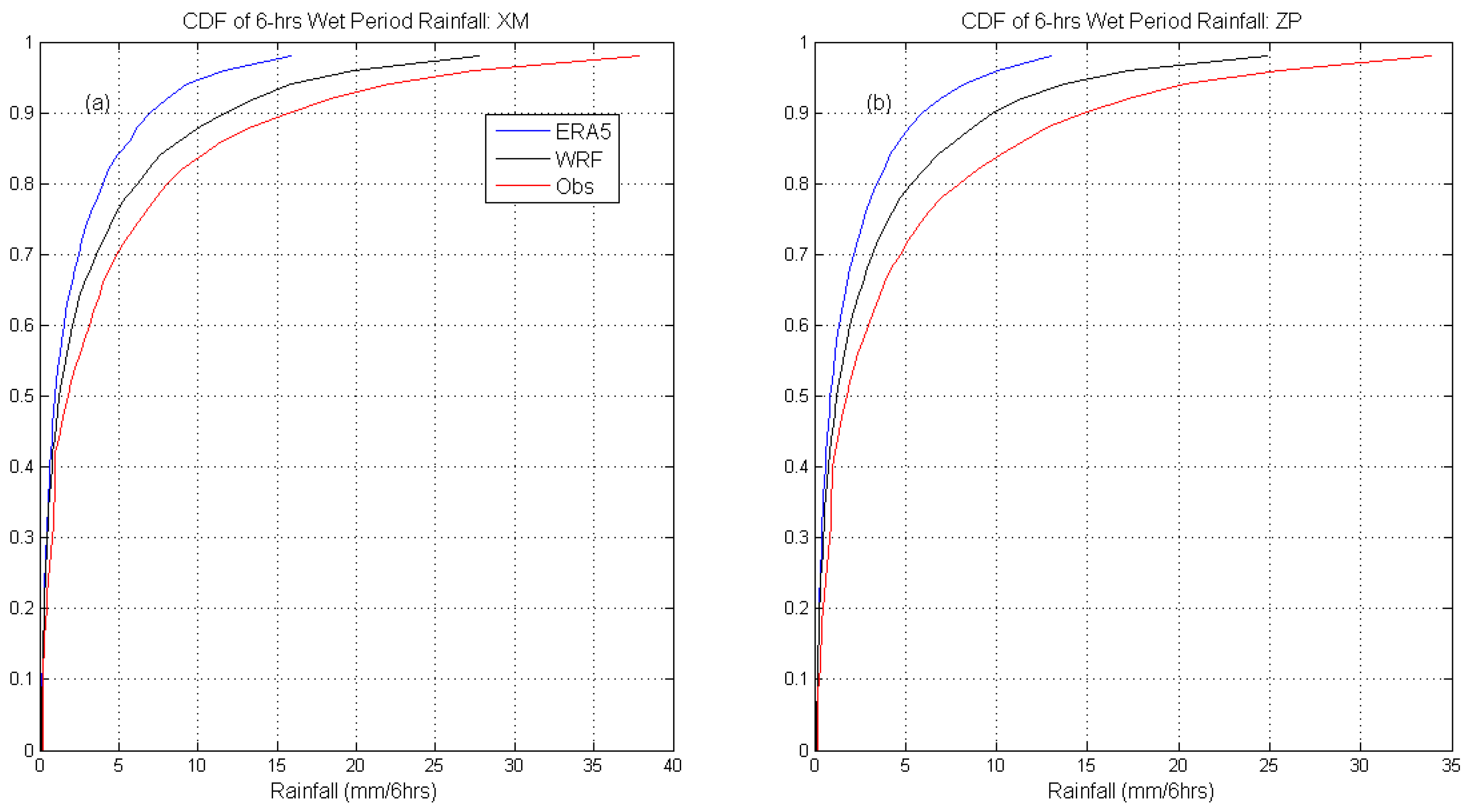
The WRF model calculates annual total rainfall amounts of 1950 mm and 2090 mm at XM and ZP, respectively, while the observed values are 1381 mm and 1694 mm, indicating relative overestimates of 41% and 24%. The ERA-5 product overestimates XM’s annual rainfall as 1656 mm (a 20% difference from observation), while it underestimates ZP’s annual rainfall as 1490 mm (a 12% underestimation). In the WRF output, the general rainfall pattern—increasing from the coast toward the inland—in southern Fujian Province is replicated. ERA5’s underestimation of inland rainfall might be attributable to the coarser spatial resolution in ECMWF’s global models, which could lead to underrepresentation of the orographic effect in the inland of Fujian Province. As the gaps in WRF outputs equate to only 5% of the data and were filled with the ERA-5 product, the dataset’s characteristics are still dominated by the WRF output. The RMSE values of the WRF rainfall amount are 6.94 mm at XM and 6.53 mm at ZP; for the ERA-5 reanalysis, the RMSEs are 5.60 mm (XM) and 5.27 mm (ZP). The WRF (ERA-5) mean bias (Mdl-Obs) of the wet period (periods during which 6-hour rainfall > 0.1 mm is observed) rainfall amount is −4.49 mm (−4.82 mm) for XM and −3.78 mm (−0.14 mm) for ZP. The underestimation of average 6-hour rainfall intensity is consistent with our expectation, as the modeled 6-hour wet periods greatly outnumber the observed, while the total annual rainfall is not proportionally overestimated. The implications of the limited accuracy of the datasets are discussed later (Section 4.2).

2.1.2. Comparisons between WRF Rainfall and ERA-5 Reanalysis Product

The consistency between the rainfall occurrences in these two datasets is compared in Table 4. The rainfall amounts are aggregated on a 6-hour basis, and a 6-hour total < 0.1 mm is defined as “dry”. The limited inherent accuracy (accurate to 0.01 mm) of the two products suggests that defining and comparing the hourly occurrence may not be very meaningful.

Table 4. Rainfall occurrence consistency between WRF and ERA5.

	ERA5_dry_XM	ERA5_wet_XM	ERA5_dry_ZP	ERA5_wet_ZP	Pct. of Agreement
WRF_dry_XM	6219	1935	---	---	76%
WRF_wet_XM	799	3435	---	---	81%
WRF_dry_ZP	---	---	4424	2733	62%
WRF_wet_ZP	---	---	598	4633	89%

The hourly collinearity of the two datasets is represented by Pearson’s R coefficient, which ranges between 0.21 and 0.28 across the selected 28 locations. Given the large sample size (74,328 samples), this indicates highly significant yet relatively weak hourly collinearity.

These comparisons suggest a moderate agreement between the two datasets. As there are not many reanalysis products with such a high temporal resolution, using ERA-5 may still be a justifiable choice.

2.1.3. Calculation of PET

Using modeled downward shortwave radiation, temperature, ERA-5 dewpoint temperature, and ERA-5 wind speed, PET was calculated. The relatively large errors in the input datasets may not justify more complex methods, so the simple Priestly–Taylor equation was adopted [30,31]. The constant $\mathsf{\alpha }$ in the equation was set at its classic value of 1.26.

An attempt was made to compute PET using the standard Penman–Monteith method. However, the final result is too small: mostly under 800 mm/year. The actual annual evapotranspiration in the catchment is about 1000 mm over the water surface and 700–800 mm over the soil surface, according to the hydrology bureau websites of the counties in the JLR watershed.

2.2. Watershed Delineation

The 90 m resolution void-filled DEM data for the study area were derived from the SRTM30 dataset. Using the TauDEM program [32] which is packaged with the HSPF program, the watershed boundary and subcatchments were delineated (Figure 3). In Figure 3a, the minimum contribution area for a subcatchment is set as 1000 km², which is used for interpolating model-output rainfall and computed evapotranspiration using the Thiessen Polygon method onto the centroids of the subcatchments (“Delineation 1”). In Figure 3b, the threshold is lowered to 100 km so that smaller tributaries can be delineated (“Delineation 2”), which was found to improve the performance of the HSPF model.

Figure 3. Two versions of watershed delineation. (a) Coarser delineation for data interpolation; (b) finer delineation for Hydrological Simulation Program-Fortran (HSPF) modeling. The three yellow subcatchments (SUB0, SUB12, and SUB4) contain the locations that are identified as crucial for runoff generation, and the WRF model output at these points (little black dots) within these sub-basins was subsequently interpolated utilizing the Thiessen Polygon method onto the centroids (red dots) of these sub-basins as HSPF input. See Section 2.4.2 “Preparing HSPF Input” for details.

The limited functionality of HSPF v12.2 (we had problems importing datasets containing more than 500,000 float numbers as input) and the large amount of data imply that only three meteorological stations (WRF grid points) can be selected in the model. These stations are assumed to be located at centroids of the selected subcatchments containing the grid points that are more critical for outflow generation. The average rainfall of the subcatchment was interpolated onto the centroid using the Thiessen Polygon method. The critical locations were first selected through MLR; the meteorological data interpolated at the centroids of the subcatchments containing these locations were further assessed for their usefulness as runoff predictors by using the ridge regression method.

2.3. Multiple Linear Regression (MLR)

We first used multiple linear regression (MLR) to identify the WRF output grid points that are critical for runoff generation. Due to this limitation, and considering that the source waters are physically important for flow generation, it is SUB0, rather than the two “critical” subcatchments (Figure 6) lying between SUB0 and SUB12 (Figure 3a), that was selected as the upper-reach critical location; as both SUB0 and SUB12 were selected through spatial auto-correlation, these two smaller subcatchments’ contributions could more or less be represented by SUB0 and SUB12. For this study, we used 28 rainfall variables as explanatory variables, and, due to the relatively close spatial distance between each precipitation grid, their performances have certain similarities, so there may be strong collinearity among explanatory variables.

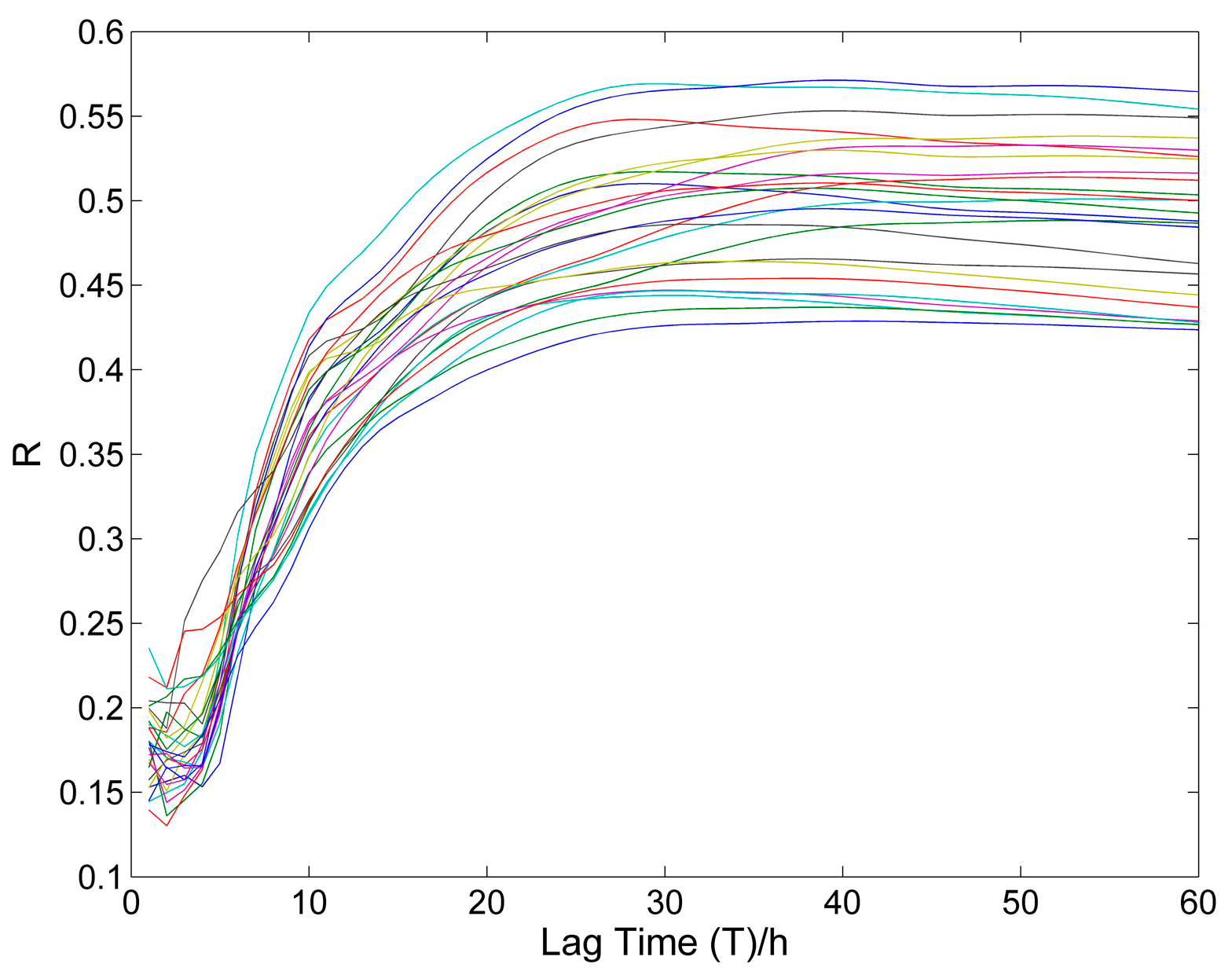
There is a lag in time from the occurrence of precipitation to the increase in the flow; this lag is referred to as the delay time. Also, the increase in streamflow is related to the accumulated precipitation during the previous time period. Hence, precipitation at different times has a different contribution to the increase in river flow. So, a weighting factor should be applied to precipitation at different times, and the selection of the weighting factor is related to the specific river basin. The following empirical formula developed for eastern New South Wales, Australia, was used to obtain the first estimate of the time of concentration according to the catchment area [33].

$$T=0.76A^{0.38}$$

(1)

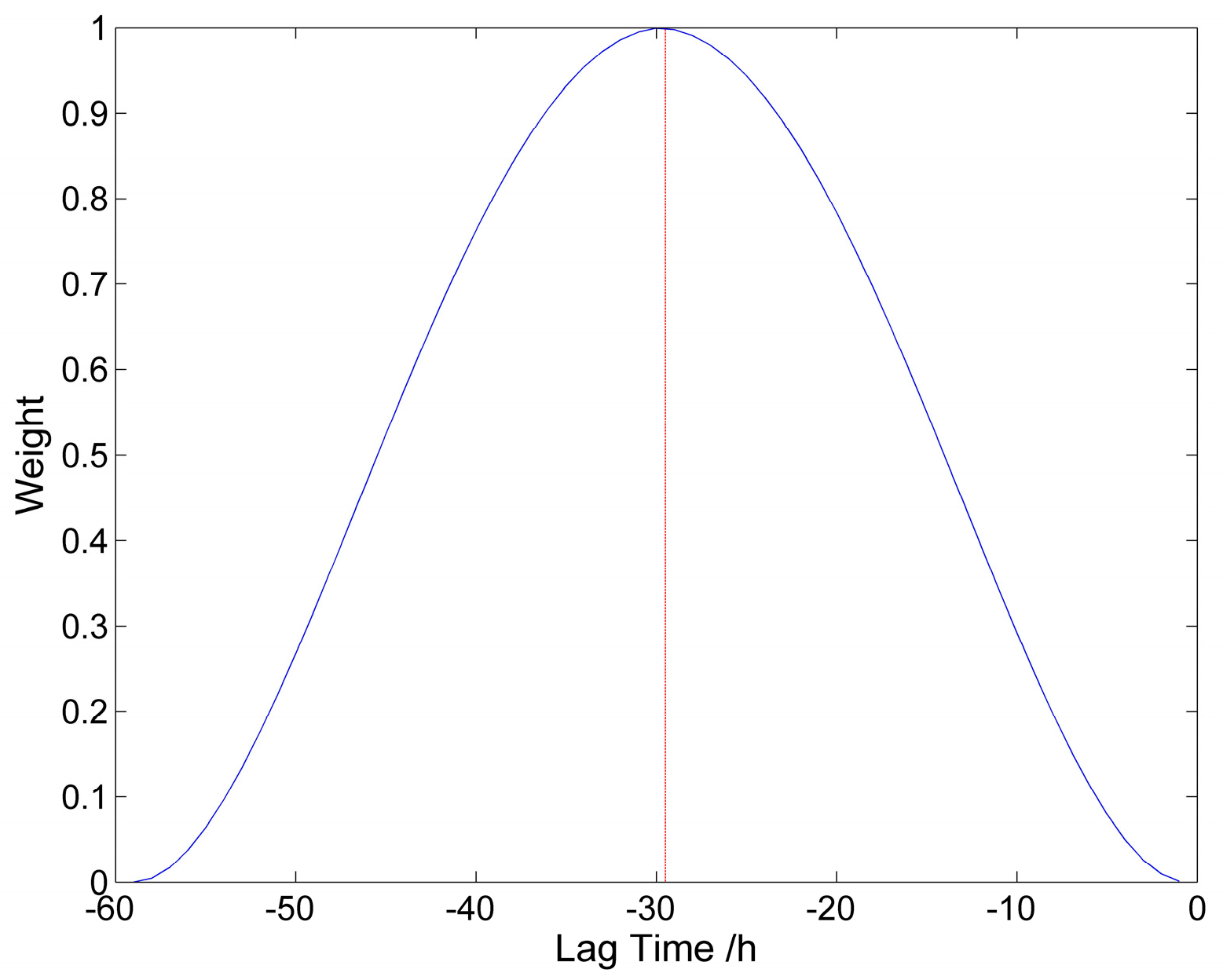
where A denotes the watershed area, and T is the delay time. This method results in an estimate of 29 h, which is quite close to the values based on lag-correlation analysis (i.e., the lag at which the correlation is maximized; most of the lines in Figure 4 reach a maximum at ~25 h and then level off) shown in Figure 4. For the weighting method, we used the bi-square function. The expression of the bi-square function is

$$W={(1-{(t/T)}^2)}^2,-T\le t\le T$$

(2)

Figure 4. The correlation coefficient of all rainfall variables against lag time.

T and W refer to the delay time at the maximum weight and the weight value, respectively, and the schematic diagram of W is in Figure 5. Given 28 locations, if the rainfall amount is temporally weighted, and a lag-time of 30 h is chosen, then for each time step, 28 × 30 = 840 explaining variables are involved. The weighting scheme can capture the temporal characteristic of the system and greatly simplify the model. The weighting kernel concept and the bi-square kernel is borrowed from the Geographical Weighted Regression (GWR) method, though, in GWR, as a weighted least-square technique, the weighting is applied to the error covariance matrix (so as to emphasize that certain observed samples are more “important/relevant” than the others). The advantage of the bi-square kernel is that the parameter T can be assigned a relatively clear and simple physical interpretation: lag time. Another widely used kernel, the Gaussian kernel, does not decay to zero beyond the maximum lag, and its bandwidth parameter cannot be so easily interpreted.

Figure 5. The weighting curve: the weight curve is shifted to the left, and the right-most value is zero, indicating the current time.

2.4. Statistical Runoff Hindcast Models

2.4.1. Ridge Regression

Based on the results from MLR, locations critical for runoff generation can be identified. To justify the three selected locations’ efficacy in predicting the discharge at the Pu’nan gauge station, and to contrive some alternative statistical models with which the HSPF model can be compared, an improved ridge regression model and a KNN model were built, solely using the meteorological data of the three sub-basins containing the critical locations (see Figure 6 and Section 2.4 for details). Ridge regression is a method widely used for dealing with high-dimensional independent variable matrices with high multicollinearity. The theories and the auto-selection of the ridge parameter can be found in the user manual of the R package “ridge” ([34]).

Figure 6. Seasonal changes in the spatial distribution of “critical locations”.

For better characterizing the temporal and spatial rainfall/evaporation patterns, some indices were constructed for the three critical locations (one near the source of the JLR, one in the middle stream, and one near the outlet; see Figure 3a). A similar design of such parameters can be found in [21], and the inclusion of certain parameters, such as the parameters accounting for the temporal and spatial distribution of rainfall, was inspired by [21].

• Total precipitation during $[T_{curr}-L-0.5L,T_{curr}-L+0.5L]$, where L is the time lag. This is an indicator of the short-term rainfall amount, and $\pm 0.5$ is included to account for the uncertainty in lag.
• Relative centroid location of the short-term rainfall hyetograph (PrecCentr). At time t_I, moving the time origin to t_I-L-0.5L, the centroid of the recent rainfall during $[t_I-L-0.5L,t_I-L+0.5L]$ is defined as:

  $$\mathrm{Pr}ecCent{r}_I=\frac{{\Sigma }_{j=1}^L{t}_{j}R(j)}{L{\Sigma }_{j=1}^{L}R(j)},0\le \mathrm{Pr}ecCent{r}_I\le 1$$

  (3)

  This is an approximate indicator of the temporal pattern of the recent rainfall. A larger PrecCentr value corresponds to more tail-loaded recent rainfall events.
• Total precipitation in the previous 30 days. This is an indicator of the “long-term” wetness condition of the system; it may have some implication for the operations of the dams on the river.
• The ratio between the previous 3-day total precipitation and previous 7-day total precipitation. This parameter describes the recent soil moisture condition in the system. For evaporation, these four parameters are computed in a similar way, except that the “centroid” is computed for the evaporation in the preceding 30 days.

Given the nonlinearity of the rainfall–runoff generation relation, the interactions between the 3 × (4 × 2) = 24 variables are also included in the model (but the quadratic of each variable itself is left out), so, in total, 300 variables were entered into the ridge regression.

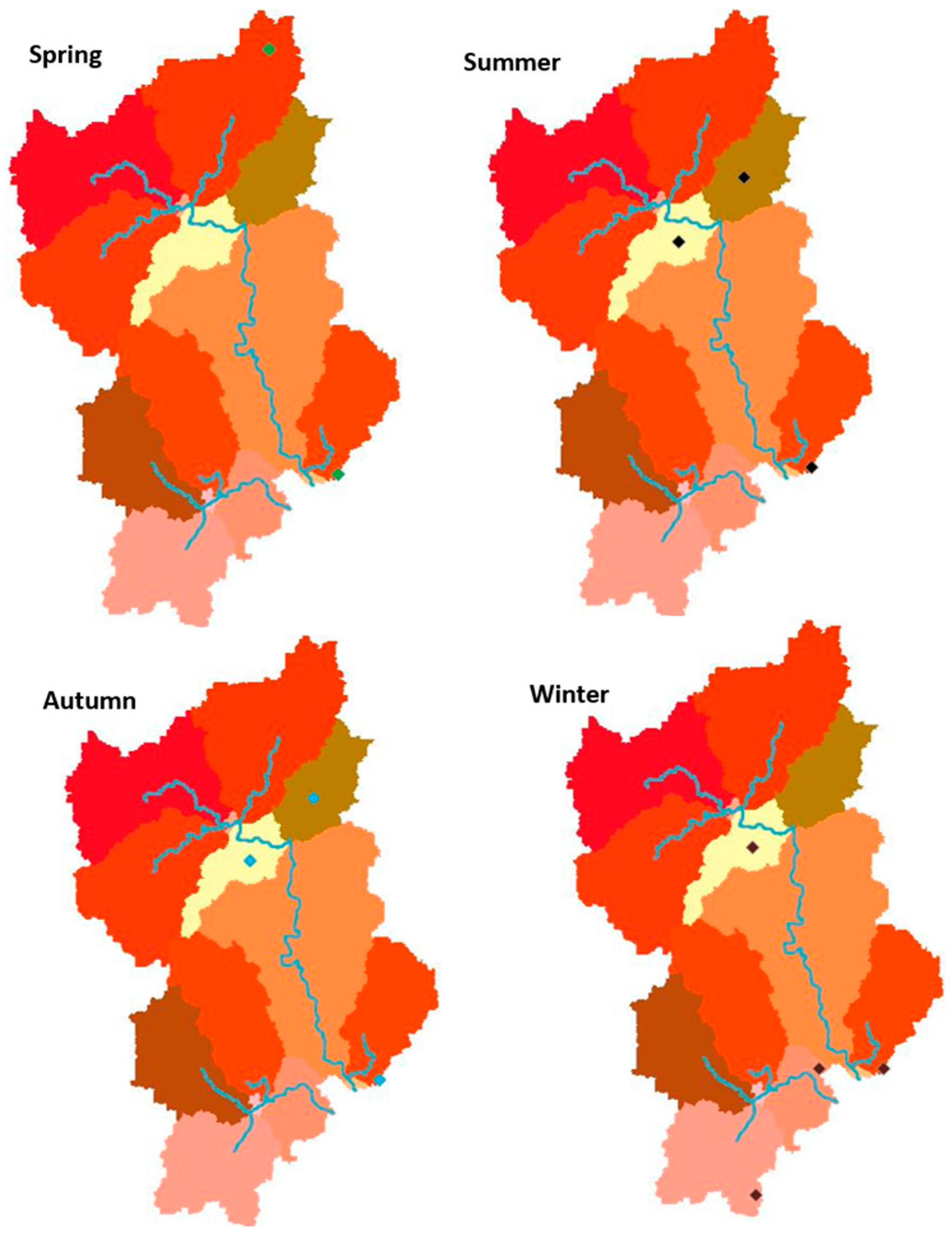
Three different configurations of the model were tested, and the above-listed parameters are those that were included in all the experiments; the experiment including only these as the explaining variables is referred to as the “Base Case”. Two more configurations were used; namely, Configurations 2 and 3. Configuration 2 is an experiment that includes the distance between the spatial centroid of the total precipitation during $[T_{curr}-L-0.5L,T_{curr}-L+0.5L]$ and the Pu’nan gauge station as an extra explaining variable. This distance is normalized by the distance between Sub0’s centroid and the gauge station, so it ranges between 0 and 1; its interactions with other variables are considered. Configuration 3 involves seasonality: as we have seen in the MLR section, the regression’s performance seems to depend on the season being modeled. Choosing Spring as the base case, three more binary dummy variables standing for Summer, Autumn, and Winter are included in the third experiment.

The daily flow rates at 08:00 were first regressed against these predictors using the linear ridge function in R’s “ridge” package. A bootstrapping procedure was applied for calibration and verification. The ridge regression was run 50 times, each time using a randomly chosen 60% (number of samples: N = 2142 × 0.6 = 1285) of the whole dataset for training, and the remaining 40% (N = 857) was used for verification. In addition to this random split between the calibration and the verification sets, the models were also calibrated using the first 60% portion of the input and validated against the other 40%; this is later referred to as “continuous hindcast”, and the previous verification is referred to as “random hindcast”. Firstly, in practice, “continuous hindcast” is a more common application of rainfall–runoff models. Secondly, for randomly split sets, it is likely that the samples adjacent to a verification data point are included in the calibration set. Given the auto-correlative nature of the datasets, predicting $y_{i+1}$ using a model trained using $x_i$ and $y_i$ might inflate the result, making it appear better than it would be if $x_i$ and $y_i$ were not in the calibration set.

2.4.2. NPRED and K-Nearest Neighbor Regression (KNN)

NPRED is an R package developed by Sharma et al. [35]. Basically, the NPRED package implements two methods: (i) nonparametric predictor identification (NPRED) using partial information (see below for expression) defined in [30]; (ii) modified k-nearest neighbor regression [10], with the samples weighted by partial weights derived from partial information coefficients (PIC) [35]. Here, the NPRED-KNN method is adopted as a nonparametric approach to statistical modeling based on kernel density estimation. More theoretical details can be found in [35] and [36]. However, these methods are highly computationally intensive (e.g., when ~50 independent variables are involved, it takes about 10 h to finish 50 runs of the NPRED-KNN algorithm using this package on a laptop with a 2.5 GHz, 4-core Intel(R) Core(TM) i7-4710MQ CPU); it is impractical to feed more than 300 independent variables into this algorithm. As an expedient solution, for each run of the ridge regression’s calibration, the variables with regression coefficients that are significant at 5% were recorded; then, the variables that were recorded at least 45 times (out of 50) were passed on to the NPRED-KNN algorithm, which was similarly run 50 times. In [9], stepwise linear regression was adopted for the similar purpose of selecting inputs for an ANN model. The division of the calibration/verification subsets and the distinction between “random hindcast” and “continuous hindcast” both follow the same logic as in ridge regression.

2.5. HSPF Model

2.5.1. Model Description

HSPF (Hydrological Simulation Program-Fortran) is a semi-distributed hydrological model developed by the Environmental Protection Agency (EPA), USA. The model simulates the surface and soil moisture in the watershed on pervious and impervious surfaces separately, and it then routes the channel flow to the outlet using kinematic wave routing (Manning’s equation is used) by estimating channel width, depth, and slope from digital elevation model (DEM) data assuming Manning’s n. The overland flow is routed into the main channel by assuming the average length and average slope connecting the pervious/impervious land surface to the channel. HSPF version 12.2 was applied in this study.

The basic inputs for the hydrological module of HSPF include meteorological data (PET; land cover types and their associated impervious percentages). Key parameters in the model include UZSN, LZSN, DEEPFER, INTFW, IRC, AGWRC, LZEPT, CEPS, etc. The first two define the nominal upper/lower zone storage of the soil; DEEPFER denotes the loss to the deep groundwater; INTFW controls how much of the direct runoff takes the form of interflow, and IRC determines interflow’s recession rate; AGWRC is the baseflow recession, which can be estimated from observation data. LZEPT is the lower zone evapotranspiration rate, which usually varies monthly according to the type and growth stage of the vegetation. More details of the model structure and routing methods can be found in the HSPF v12.2 user manual [37].

Due to the lack of high-quality land use and groundwater survey data, the model calibration started with recommended values of the parameters and estimated AGWRC (0.985–0.992 based on the baseflow separated from the observation). The calibration was done manually, guided by data analyses and the recommended parameter ranges in [38], and the result is expected to be only a very crude approximation of the actual parameters.

2.5.2. Preparing HSPF Input

HSPF 12.2 is distributed with free hydrological GIS software, TauDEM [32]. The sub-basins and the stream link network can be automatically delineated using TauDEM. Then, each sub-basin is assigned the meteorological station closest to its centroid (referred to as “Model Segmentation”).

As mentioned in Section 2.4, due to the large amount of the hourly input data (~8.5 years, 74,328 h), no more than three “meteorological stations” (i.e., the locations where we have WRF outputs) can be selected in our application. To overcome this limitation and achieve a balance between reducing the amount of data and describing the spatial heterogeneity in rainfall, three sub-basins in Delineation 1 (Sub0, Sub4, Sub12) that contain the critical locations were selected, and their sub-basin-scale average rainfall/PET were computed by interpolating the data points within them using the Thiessen Polygon method. A more relevant approach for such a mountainous area may be Krigging regression, which may account for the elevation and the sloping direction of a pixel, yet we only have 28 spatial grids, making the training of such a model impractical. Other non-regression methods may share the same problem with the Thiessen polygon; to keep things simple, we stuck to this method for this study.

From MODIS and GMIS data, we estimated the areal proportion of each land cover type and impervious percentage of each land cover type. Each pixel in the MCD12 product (labeled with a certain type of land cover) measures 500 × 500 m²; there are about 278 GMIS pixels, which are 30 × 30 m² each. Each GMIS pixel is labeled as pervious or impervious, so the impervious percentage of such a MODIS pixel can be estimated. Thus, on a subcatchment or whole-catchment scale, the total impervious percentage of the (sub)catchment and the average impervious percentage of each land cover class (assuming all the samples for computing this average come from the same population, and the standard deviation of the estimate of this average can also be estimated) can be derived. In total, impervious surface accounts for 19% of the whole watershed area; the average impervious percentage of each land cover type is shown in Table 5.

Table 5. Land cover type.

	Proportion	Imp
Water body	0.08%	33% ± 88% (n = 42)
Permanent Wetland	0.01%	Unavailable from GMIS
Forest	37.98%	15% ± 5% (n = 20,308)
Grassland	55.56%	22% ± 0.4% (n = 29,709)
Cropland	4.34%	14% ± 2% (n = 2325)
Urban	2.02%	40% ± 2% (n = 1079)

Note that this is only a very rough estimate of the proportion of the impervious surface. Some data presented here are not consistent with previous studies [1,39], e.g., overestimation of grassland coverage. The impervious percentage for water body in Table 5 is obviously unreasonable. In our application, it could either be set to 0 (artificial lakes, etc. that do not drain into the JLR) or 1 (dams and channels belonging to the JLR stream network). Since it is a very small proportion of the whole watershed area, setting it to 0 or 1 is not likely to have significant impacts, so here it was set to 0.

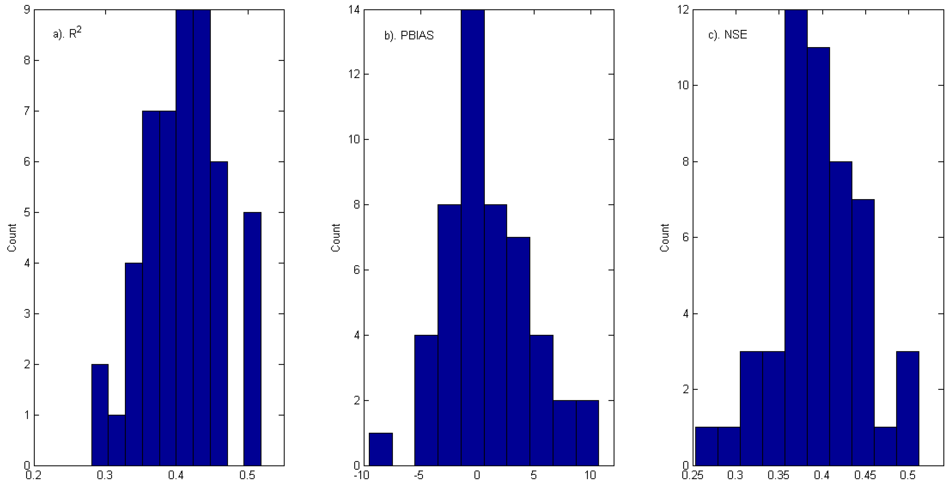
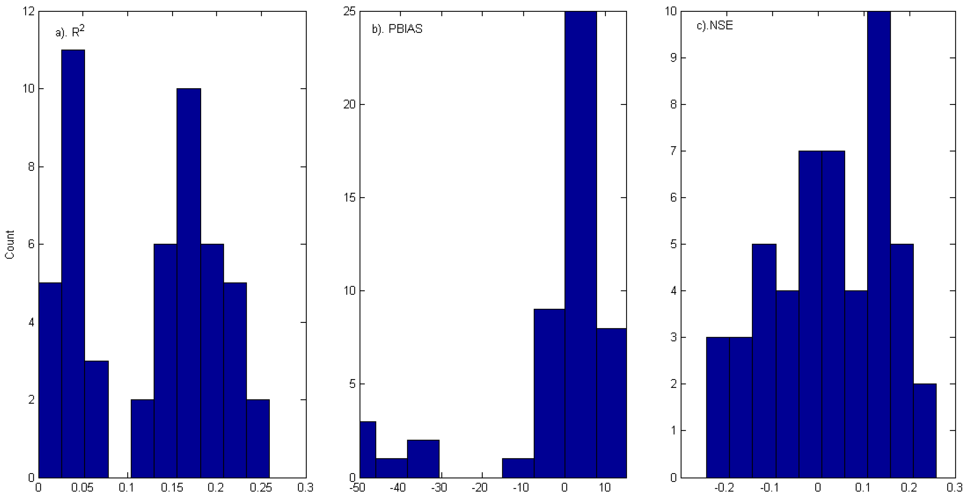
2.6. Verification Methods

The models were assessed using R² (Equation (4)), the Nash–Sutcliffe model skill (NSE), and the percentage bias (PBIAS; Equation (6)) from [40], as some empirical guidelines on their interpretations were proposed in [40], and, at this stage, we do not particularly focus on low/high flow characteristics, for which log-transformed/squared error statistics may be preferred:

$${\mathrm{R}}^2={\left[\frac{{{\displaystyle \sum }}_{i=1}^N(Y_i^{mdl}-\overline{Y_{}^{mdl}})(Y_i^{obs}-\overline{Y_{}^{obs}})}{{({{\displaystyle \sum }}_{i=1}^N{\left(Y_i^{mdl}-\overline{Y_{}^{mdl}}\right)}^2)}^{0.5}{({{\displaystyle \sum }}_{i=1}^N{\left(Y_i^{obs}-\overline{Y_{}^{obs}}\right)}^2)}^{0.5}}\right]}^2$$

(4)

$$\mathrm{NSE}=1-\frac{{{\displaystyle \sum }}_{i=1}^N{\left(Y_i^{mdl}-Y_i^{obs}\right)}^2}{{{\displaystyle \sum }}_{i=1}^N{\left(Y_i^{obs}-\overline{Y_{}^{obs}}\right)}^2}$$

(5)

$$PBIAS=\frac{{\Sigma }_{i=1}^N(Y_i^{mdl}-Y_i^{obs})}{{\Sigma }_{i=1}^N{Y}_i^{obs}}\times 100\%$$

(6)

The models were assessed according to the guidelines in [40], in which, for streamflow, a “satisfactory performance” is defined as NSE > 0.50 and PBIAS within $\pm 25\%$. In some references ([14]), for daily flow rate, a necessary condition for satisfactory model skill is R²$\ge$0.6.

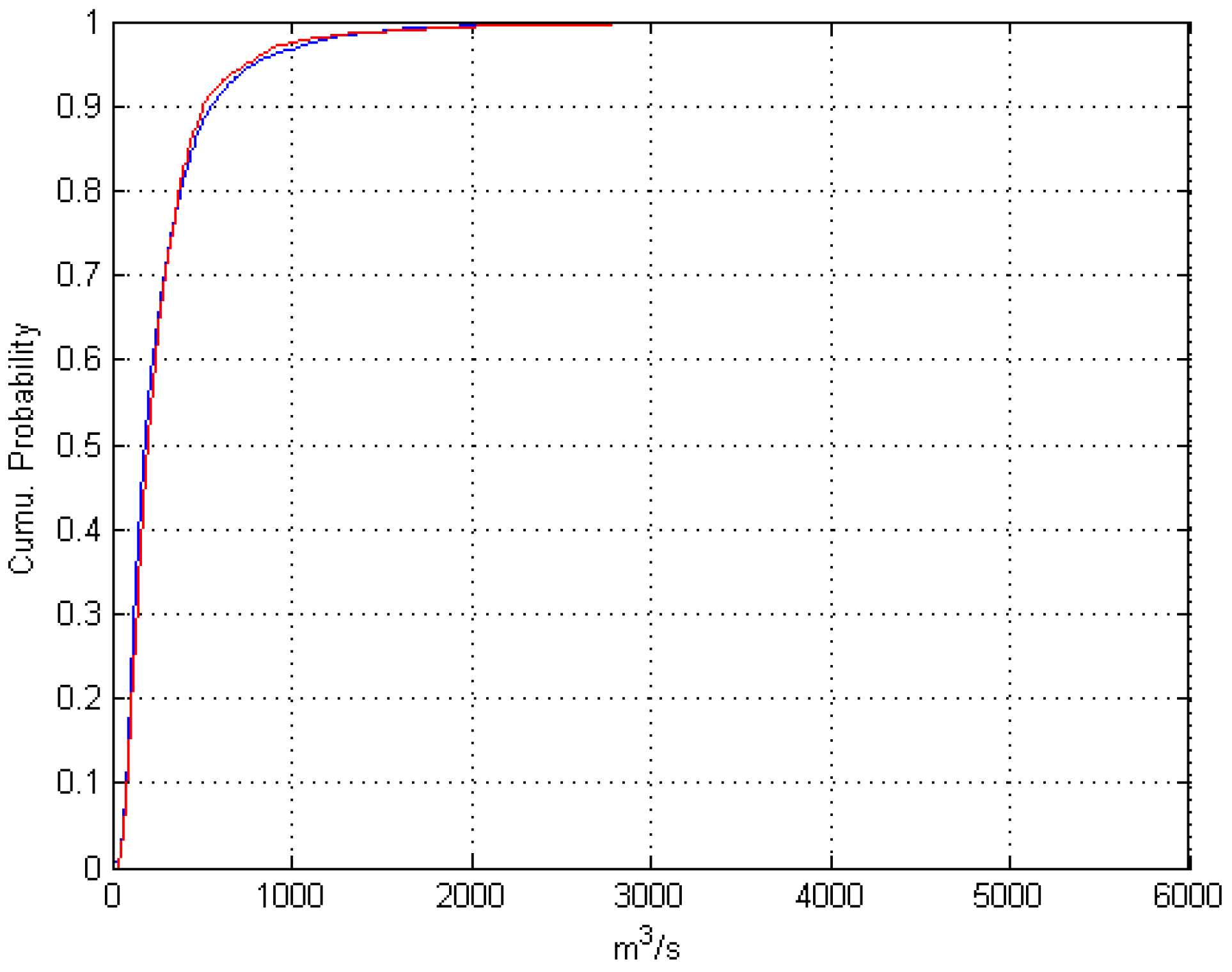
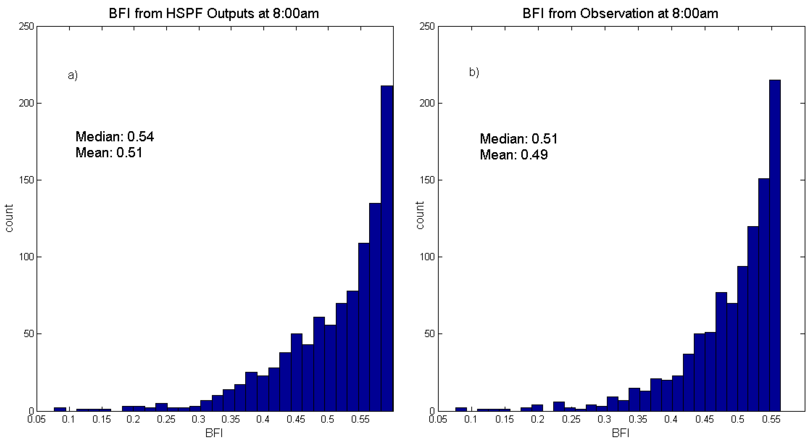
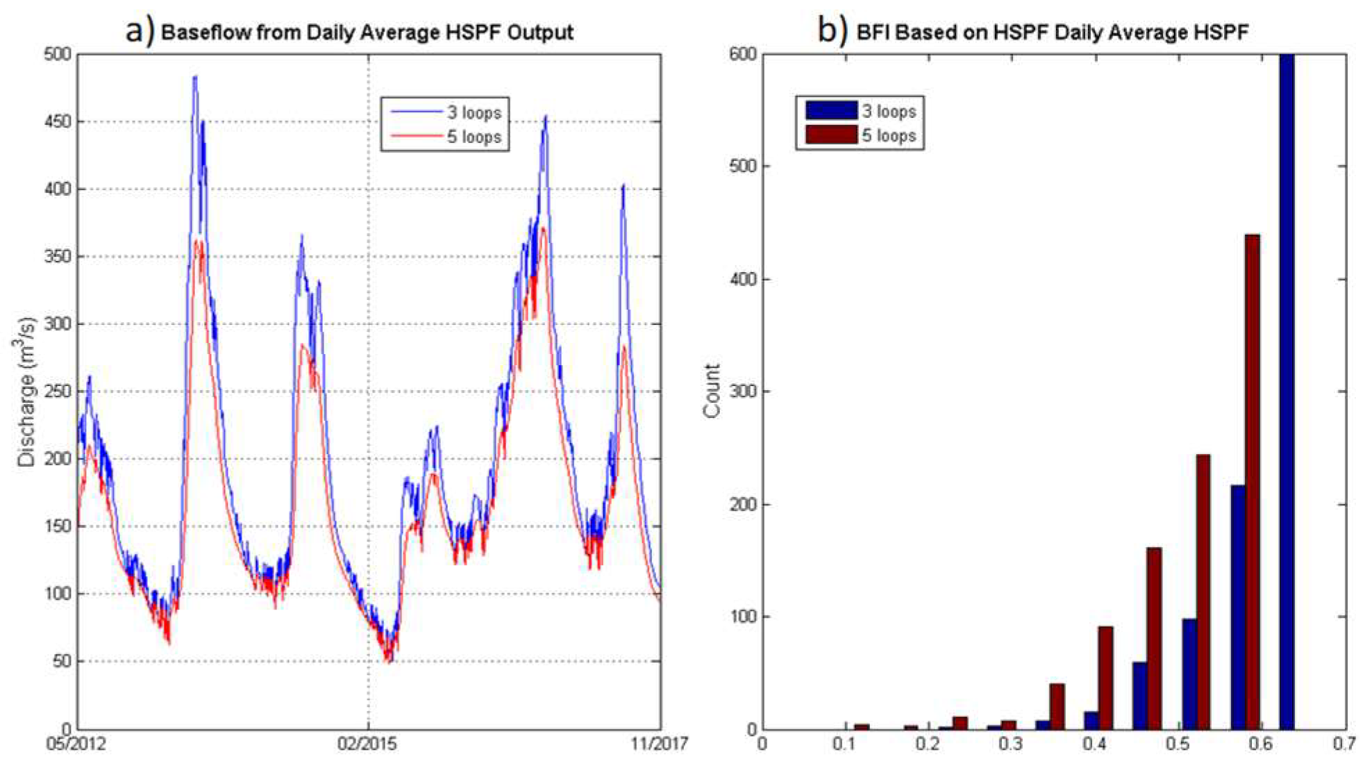
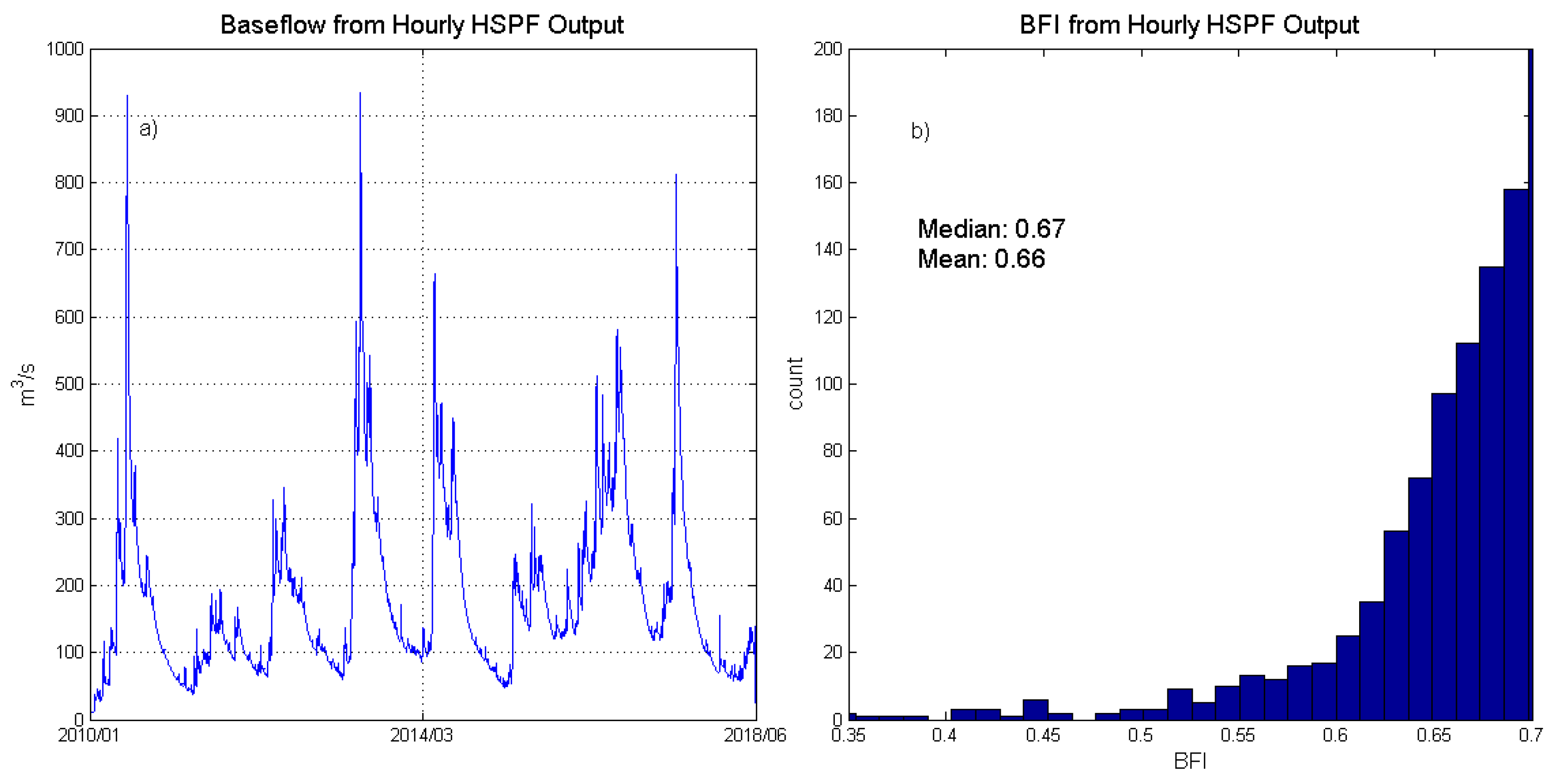
For HSPF model output, the baseflow index (BFI) was also computed and compared with the BFI estimated from the observation data. The computation of BFI follows the method introduced in [41], where the Hollick filter algorithm is applied 1000 times, each time using a filter parameter randomly chosen from [0.9,0.99], and the final BFI estimation is taken to be the median or the mean of the 1000 runs; each run consists of applying the filter to the flow rate data in alternate directions for an odd-number of times (n=3,5,7,… “loops”). In [41], it is recommended that the algorithm is looped for 3 times (n = 3) if the daily flow rates are used and for 9 times (n = 9) if the hourly input is involved. This overcomes the difficulty of filter parameter selection in the conditional method, where only one single run of filtering is implemented, and the method in [41] could reduce the uncertainty associated with filter parameter selection through averaging. The authors in [42] suggest choosing filter parameters on the basis of expert geological knowledge of the study area, and that parameters thus chosen can outperform those selected by machine learning techniques (since they attempt to optimize total outflow at the cost of less realistic baseflow estimation); however, due to the limited access to the geological data of the region, we preferred to keep the approach more data-driven at this stage. HSPF output will be aggregated using different methods ((i.) Daily average; (iii.) Hourly raw output) before the computation of BFI, and the n value’s and the aggregation method’s impacts on the estimated BFI will be briefly discussed.

3. Results

3.1. MLR

A comparison of the three delay methods is shown in Table 6.

Table 6. Comparison of the three delay methods.

Delay Method	No Delay	Point Delay *	Bi-Square
R2	0.0116	0.1744	0.4088

* means the correlation between the runoff and the precipitation of previous time steps but no weighting is applied.

It can be seen from Table 6 that the explanatory ability of precipitation regarding flow is significantly improved by using the bi-square weighting method. We also used the VIF (variance inflation factor) test method to check multicollinearity; generally, VIF > 10 is deemed to indicate strong collinearity, and the results show that only two variables have a VIF value of less than 10, so the collinearity is strong. However, the regression here is part of a preliminary investigation, so the problem of collinearity is not rectified for the time being.

Also, the explanatory ability of rainfall may vary for different seasons, so we conducted MLR for the four seasons, individually. By comparing the corresponding R² of the four seasons, the contribution of precipitation to runoff in each season was determined. The results are shown in Table 7.

Table 7. R² for different seasons.

Season	Spring	Summer	Autumn	Winter
R2	0.3875	0.5136	0.3411	0.2347

According to Table 7, the values of R² for summer and spring are larger, while those for autumn and winter are smaller. It suggests either that in different season the mechanism of runoff generation is different (which is possible, given the classical “variable source” hypothesis and the size of the catchment) or that the over-predicted rainfall occurrence and under-predicted intensity are more detrimental to the MLR predictions of Spring and Winter runoff. This indicates that, in different seasons, the mechanism of runoff generation differs. MLR’s inadequacy in modeling slow-varying baseflow may be on account of its poorer performance in winter and spring (i.e., the relatively dry seasons). The baseflow index (BFI) was subsequently calculated from the observation and HSPF output, as shown in another section.

Based on this regression, different variables have different significance levels, so, for each season, we selected variables with a high significance (p < 0.01), as shown in Figure 6.

The seasonal variability in the selected locations (based on the p-value) seems to reflect the concept of the variable source [43,44], though further catchment-scale investigation is required. To distinguish the results here from those obtained for a well-established variable source framework, for the time being, we do not refer to these locations as “hydrologically sensitive areas”; rather, we call them simply “critical locations”.

3.2. Statistical Models: Ridge Regression and NPRED-KNN

3.2.1. Ridge Regression (RR)

The verification results—both “random” verification and “continuous” verification—of the three model configurations are shown in Table 8.

Table 8. Performance metrics of the ridge regression (RR) models---Verification period (numbers outside of brackets are the medians of 50 random verification runs (for PBIAS, the minimum, maximum, and the median are listed); bracketed numbers are metrics of the continuous verification).

	R2	PBIAS (%)	NSE
Base Case	0.41 (0.46)	−9.51, 10.71, median = −0.38 (−10.92)	0.40 (0.42)
Config 2	0.41 (0.47)	−9.59, 10.92, median = −0.49 (−11.19)	0.40 (0.42)
Config 3	0.41 (0.46)	−9.50, 10.73, median = −0.40 (−11.46)	0.40 (0.41)

The three configurations make little difference in regard to the three performance metrics. None of them yield a set of satisfactory metrics (R² > 0.6, NSE > 0.5, |PBIAS| < 25%), and the RR method systematically underestimates the flow rates by ~10% in the continuous verification. The time series hindcasted by RR is plotted in Figure 8. As different configurations display similar skills, only the Base Case configuration is further examined and discussed, as it is the simplest configuration of the three.

The histograms of the three metrics, based on the random verification runs, are shown in Figure 7 for the Base Case.

Figure 7. Histograms showing R², PBIAS, and Nash–Sutcliffe model efficiency (NSE) of the “random verification” of Configuration 3.

For the Base Case, the independent variables whose regression coefficients are significant for over 90% of the random verification runs (at least 45 out of 50) were selected as the critical ones. They were used as input predictors for the KNN model, and a smaller ridge regression model, RR2, was constructed using them as explaining variables. In total, 35 out of 325 variables were selected. The verification performance metrics are listed in Table 9.

Table 9. RR2’s verification performance (daily, n = 857).

	R2	PBIAS (%)	NSE
RR2 Model	0.44 (0.50)	−9.16, 9.87, median = −0.59 (−10.92)	0.42 (0.44)

Compared with RR’s metrics in Table 8, the model performance metrics in Table 9 are slightly improved, though the flow rates are still systematically underestimated. The verification results of RR, RR2 outputs, and observations are graphed in Figure 8. Visual inspection suggests that there is a severe underestimation of the peaks, whilst the timing of the highs and low and the shape of the recession limbs are better represented than the magnitudes. Further investigation shows that, when RR2’s verification outputs are multiplied by a factor of 1.10, the PBIAS (NSE) then decreases (increases) to −3.3% (0.47). This suggests that RR2’s verification outputs are likely to be dominated by systematic errors.

Figure 8. The hindcasts made by ridge regression models are compared with observations.

For the RR2 model, the flow rates hindcasted in continuous verification were block-averaged over 30-day window lengths and compared with the block-averaged observations. On this monthly timescale (n = 38 samples), R² = 0.65, PBIAS = −15.32%, and NSE = 0.53 (Table 10). As expected, the systematic underestimation persists, while the other two metrics improve, probably because the sample size becomes much smaller. We also attempted to generate an hourly hindcast using the RR2 model; however, doing so resulted in a large number of negative values. This is possibly attributable to the fact that the model was trained using a relatively small training set (~1200 samples), whilst the hourly test set comprises ~20,000 samples, many of which might contain variable combinations unseen during the training.

Table 10. RR2’s verification performance (continuous, monthly; n = 38).

	R2	PBIAS (%)	NSE
RR2 Model	0.65	−15.32	0.53

3.2.2. NPRED-KNN

The 35 selected predictors of the Base Case were fed into the NPRED-KNN algorithm, but this method performs badly in verification. The median NSE of the 50 “random hindcast” runs is only 0.02, and the maximum is 0.26 (Figure 9); R² is always smaller than 0.30, and the underestimation could be as high as 50%. This may suggest that the candidate variables preliminarily selected by RR are not suitable for KNN or that KNN itself is inferior to RR in this application. For “continuous hindcast”, the NSE of the KNN method is only −0.04, and R² is 0.07, again indicating that the method might be inappropriate.

Figure 9. R², PBIAS, and NSE of 50 “random hindcast” runs of k-nearest neighbor (KNN) model.

We may conclude that the RR method outperforms the NPRED-KNN model when the 24 variables and their quadratic interaction terms are entered as predictors. However, the attempt to simulate hourly runoff using the RR or RR2 model fails due to the large number of hindcast negative values. This is not very surprising, given the small training set (N = 1285) relative to the large number of scenarios required in the output (more than 70,000 h); many of the scenarios (i.e., combinations of input variables) may be absent from the training set, so the model could generate unrealistic predictions in this case. In later sections, the RR (RR2) model is excluded from discussions involving hourly output.

3.3. HSPF Hydrology Model

The NSE, PBIAS, and R² of each year are listed in Table 11. For the first 3 years, the model’s poor performance is attributable to the inaccurate specification of the initial condition, of which we have very limited knowledge. Excluding the first 2 years, the overall NSE is 0.36, R² is 0.38, and PBIAS is 1.41% for 2012–2017.

Table 11. HSPF model statistics.

	2010	2011	2012	2013	2014	2015	2016	2017 *	2016–2017	2010–2017	RR’s Verification Period
NSE	−0.01	−1.05	0.11	0.31	0.29	0.22	0.43	0.45	0.45	0.25	0.42
PBIAS	−11.26	−12.21	−14.80	17.09	26.91	−15.03	−7.95	4.41	−3.25	−1.45	−1.10
R2	0.31	0.06	0.27	0.53	0.53	0.24	0.44	0.46	0.46	0.38	0.43

* 2017 refers to the period from 01 January 2017 to 30 September 2017.

Figure 10 displays the simulated and the observed flow rate time series, and Figure 11 shows the comparison between the empirical cumulative distribution functions derived from the modeled and the observed daily (08:00) flow rates. The observed average runoff over the simulation period is 283 m³/s, and its modeled counterpart is 279 m³/s, differing by 1.4%. For the average of the lower 50% flow rates, the model has a −8.91% relative error (111.85 vs. 122.79 m³/s), and the model overestimates the top 10% flow by 1.84% (983.12 vs. 965.39 m³/s).

Figure 10. HSPF model output and observations. The top panel shows the modeled and observed 6-hour total precipitation at Zhangping.

Figure 11. Cumulative distribution of daily 08:00 flow rate of simulation and observation.

The observed values and the model output were also block-averaged on a 30-day scale (a proxy for ‘monthly’ average runoff). The relevant statistics for the 30-day-averaged values of the RR model’s verification period are summarized in Table 12.

Table 12. HSPF model skill for monthly average runoff.

R2	PBIAS	NSE
0.63 (n = 95)	−3.9%	0.60

When the baseflow separation algorithm described in [41] was implemented on both the model output and the observations, we easily notice that the model can accurately replicate the BFI (baseflow index) of the observations (Figure 12).

Figure 12. Baseflow index computed from daily 08:00 HSPF output and observations.

We may conclude that this empirically calibrated HSPF model is only capable of replicating the monthly average runoff and the slow-varying, long-term baseflow pattern. Seong et al. [12] reported a framework for combining HSPF with a Shuffled-Complex Evolution algorithm (SCE-UA) [45] through programming in R. SCE-UA can efficiently help avoid the problem of being trapped in a local optimum. However, Table 9 in [14] also suggests that the auto-calibrated models may not necessarily have better performances than the manually calibrated ones.

4. Discussion

4.1. Baseflow Index (BFI)

The baseflow index computed using the method in [41] is sensitive to the number of times the input data are filtered. In [41], it is recommended that the algorithm is looped three times (n = 3) if the daily flow rates are used and nine times (n = 9) if hourly input is involved. However, in Figure 13a, we can notice that, if daily input is utilized, the separated baseflow time series is still ragged when n = 3, and the curve becomes reasonably smooth when n = 5. For hourly inputs (Figure 14), when n = 9, the separated baseflow already looks reasonably smooth. The BFIs computed using different n values and different timescales are reported in Table 13. Hourly input with n = 9 yields an estimation consistent with the case where daily input and n = 3 are used (BFI ~0.60), yet, when n is increased, at least for the daily inputs, the BFI decreases. The selection of n could still be subjective, depending on the user’s judgment concerning whether the separated baseflow is “smooth” enough.

Figure 13. Baseflow extracted from daily averaged HSPF output, looping three times (blue) or five times (red) using the method introduced in [41]. When the loop number is set as 3, the separated baseflow still looks ragged, possibly contaminated by the “quick flow” (i.e., overland streamflow).

Figure 14. Baseflow extracted from hourly HSPF output (a) and the BFI estimated from the hourly output following the method in [41] (b).

Table 13. Baseflow index (BFI) computed from hourly and daily streamflow simulation.

	HSPF (Daily), n = 3	HSPF (Daily), n = 5	HSPF (Hourly), n = 9	Obs, n = 3	Obs, n = 5
Median of BFI	0.62	0.54	0.67	0.60	0.50

In [46], the authors constructed a global map of BFIs based on the observations from 3394 catchments utilizing a 1-hidden-layer artificial neural network. According to this map (Figure 11 in [46]), the BFI of our catchment lies between 0.45 and 0.65. Almost all the values listed in Table 13 roughly fall into this range (only the 0.67 associated with n = 9, hourly input lies slightly out of this range). However, according to Huang’s research in [47], using daily flowrate data, the BFI of JLR catchment is found to be greater than 0.70. More experiments, both in-situ fieldwork and numerical experiments, may be required for determining the actual BFI of the catchment.

4.2. Implications of the Inputs’ Data Quality: A Brief Qualitative Discussion

As mentioned in Section 2.1.1, the average 6-hour wet period rainfall is underestimated in both the WRF and ERA5 datasets. The empirical cumulative distribution functions (ECDFs) shown in Figure 15 illustrate more clearly that the rainfall intensity is underpredicted by the model outputs across all the percentiles (0–98%). This, combined with the more frequent rainfall occurrences in the two model datasets, may partly explain why the modeled flood peaks are often underpredicted, and why the minor peaks between two major storm events arise more frequently in the hindcast than in the observations. The underprediction in the RR2 model seems to be more systematic, as it could be greatly alleviated by multiplying the RR2 output with a factor of 1.10, thus bringing down PBIAS to −3.3% and increasing NSE from 0.44 to 0.47. For the HSPF hindcast, the lower PBIAS and lower NSE suggest that the errors might be more random: the over/underestimations tend to cancel each other out, while the hindcast generally deviates severely from the true values (thus the low NSE).

Figure 15. The rainfall intensity empirical cumulative distribution functions (ECDFs) (covering the range of 0–98%) comparing 6-hour wet period model outputs with observations: (a) XM; (b) ZP.

Given the large deviation of the modeled rainfall from the real-world observations, the “best” selected parameters could be different from those that might be inferred from the real-world physical properties (e.g., experimentally determined soil hydraulic conductivity, etc.). From a Bayesian point of view, this might suggest that, when the model calibration is guided by some empirical values (e.g., initializing the parameter prior distribution with a mean located at the empirical value), the underlying distribution should take a large variance to account for the large uncertainty induced by the model rainfall’s deviation from the real world; with properly designed priors, algorithms such as Markov-Chain Monte Carlo (MCMC) [48,49] may then be implemented.

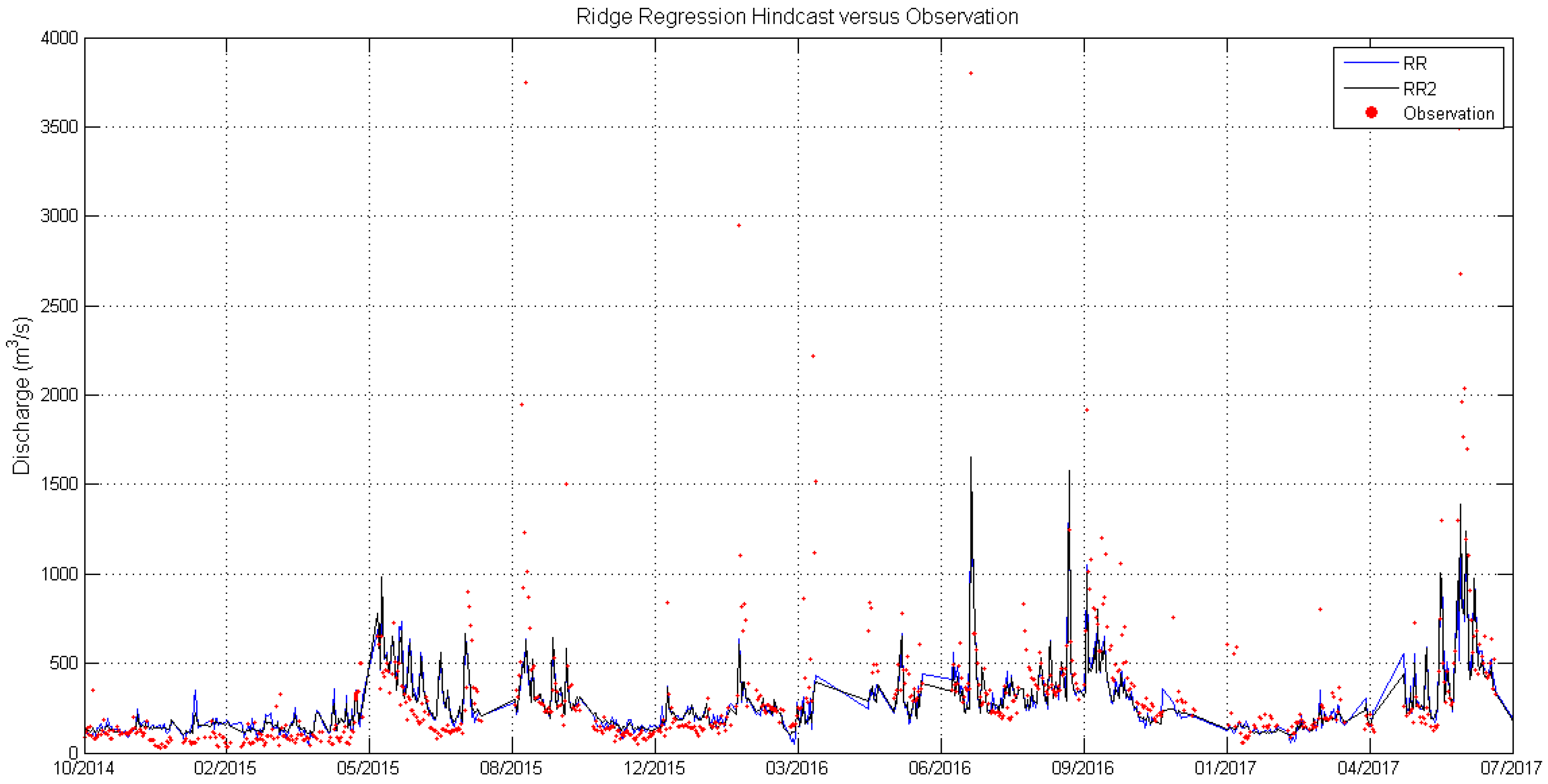
5. Conclusions

The verification performances of the “simplified” RR model (RR2) and the HSPF model outputs are summarized in Table 14. For the data-scarce catchment in the present study, the ridge regression (RR) model with appropriately constructed variables describing rainfall intensity, evaporation, antecedent watershed moisture, and month/season seems to perform no worse than a semi-distributed HSPF model. However, the RR method (1) seems to be more susceptible to systematic biases (~10% underestimation of streamflow) than HSPF; (2) fails to produce realistic hourly runoff, whilst HSPF does not have this problem, as it is physically based; (3) has regression coefficients and systematic bias characteristics that may not be stationary over time, so it is not suitable for scenario studies. The NPRED-KNN method produces very poor results, which may suggest that the training set is not big enough, or the independent variables designed by the authors in this work are unsuitable for the NPRED-KNN method. We may tentatively suggest that the hourly outputs of HSPF are still acceptable and realistic (though not “satisfactory” by the standards set by thresholds for performance metrics); it may be meaningful to use them as inputs into certain ocean models for scenario studies, though care should be taken and more analyses (e.g., errors in the timing of the peaks) are required.

Table 14. Comparing the RR2 and HSPF models (verification period).

		R2	PBIAS	NSE
Daily	RR2	0.50	−10.92	0.44
	HSPF	0.43	−1.10	0.42
Monthly	RR2	0.65	−15.32	0.53
	HSPF	0.63	−3.90	0.60

The HSPF model appears to be successful at replicating the JLR system’s baseflow index, yet the parameter selection for the BFI computation algorithm outlined in [41] could introduce some uncertainty into the final results. Depending on different parameter selection strategies, the estimated BFIs using daily/hourly flow rates could either be consistent or inconsistent with each other, though it might be determined that the BFI of the JLR catchment lies in the range of 0.50–0.67, agreeing well with [46].

The major limitations of the present work include (1) the “black box” nature of the RR model, which renders it unfit for scenario studies; (2) the limited sources of input and observation data, which results in input data that are not very accurate, and the hourly outputs of HSPF could not be adequately verified against hourly observations; (3) the problem with using HSPF v12.2 for importing large input datasets; an expedient measure was taken as a workaround, and, in the future, the feasibility of some similar models will be assessed; (4) inadequate quantitative analyses of input data inaccuracy’s impact on the modeled streamflow.

In the long term, the data sources can be ultimately diversified, and their accuracy and quantity should be improved. In the short term, when the input data’s quality still lies at the core of our problem, techniques such as MCMC (mentioned in Section 4) may be employed to account for the large uncertainty in the parameters. Some proposed alternatives for improving the rainfall data accuracy can also be adopted: (i) spatially interpolate the meteorology station data that we have; (ii) further statistically downscale model outputs (e.g., GP, SLP, etc.) to local rainfall [50]; (iii) the forecast of intense rainfall associated with typhoons remains a challenge due to the large uncertainty and long lead time [51], though estimating rainfall distribution and intensity from posterior probability distributions derived from satellite data has proven useful [52]. For (i), observation data availability is a major challenge: from various sources (e.g., www.rp5.com.ru, National Ocean and Atmosphere Administration (NOAA)’s websites), only 2–3 stations in the JLR catchment area are available for downloading, making interpolation and its validation unfeasible. The limited data availability also poses a problem to training the downscaling model in (ii). In the short term, when the issue of data scarcity persists, the more feasible option for improving the rainfall forecast seems to be (iii). However, beware that the WRF model may still require much refining; otherwise, the posterior distribution derived from the WRF-simulated rainfall and satellite measurements could still deviate severely from observations because, currently, the WRF prediction of rainfall occurrence seems to be systematically biased.