Abstract
Cellular automata (CA) modeling is a powerful and efficient tool for simulating the dynamic evolution of polycrystalline microstructures in modern materials and metallurgy studies, such as solidification, plastic deformation and recrystallization. We propose a novel model to calculate the shape factor of grains in three-dimensional hexagonal grid (3D-HEX) CA, which overcomes the disadvantages of 3D-HEX CA, such as complex algorithms and a long computation time. The shape factor is a quantitative measure of grain morphology based on the ratio of the surface area of the grain to its volume-equivalent-sphere and volume-equivalent-chain. It indicates how the shape of a grain or phase affects its mechanical properties, such as stiffness, deformation and fracture. Our model can easily calculate the shape factor for any grain by counting its surface cells and volume cells. We test our model on 1000 grains with different shapes (equiaxed, irregular and chain-like) by Monte Carlo (MC) methods. MC methods evaluate the validity of a calculation model by comparing the simulated outcomes with the observed or expected outcomes. The results show that our model can accurately describe the grain morphology and has a good comparability and generality.
Keywords:
shape factor; cellular automaton; 3D hexagonal grid; Monte Carlo; modeling; microstructure 1. Introduction
Cellular automata (CA) modeling is a powerful and efficient tool for simulating polycrystalline dynamic microstructure evolution in modern material and metallurgy studies, such as solidification, plastic deformation and recrystallization [1]. In recent years, CA have been applied to various material science problems involving complex topological changes at different length scales [2,3,4]. Some examples include recrystallization phenomena, eutectic transformation during solidification, phase-field modeling of dendritic growth, fracture mechanics, corrosion processes, etc. These applications demonstrate that CA can capture the essential physics of materials’ behavior with a high computational efficiency and flexibility [5,6,7,8].
For example, the model of a cellular-automata simulation of the grain growth of a powder metallurgy Ni-based superalloy [9] incorporates thermodynamic and kinetic mechanisms to describe the microstructural evolution of a Ni-based superalloy during hot isostatic pressing. The model can predict the grain-size distribution, grain-boundary migration velocity and grain-boundary energy under different processing conditions. A cellular-automata model for modeling phase-change materials [10] describes the temperature distribution and phases (liquid/solid) evolution for multi-component materials with a complex geometry. The model can handle phase-change phenomena, such as melting, solidification, latent heat storage and release. These research outcomes show that CA modeling is a versatile and promising technique for studying various aspects of materials science at different scales.
CA modeling, especially on a two-dimensional square grid (2D-SQR), is widely used to describe or predict microstructural characteristics [11]. The spatial discretization used by 2D-SQR can sometimes produce unnatural anisotropic patterns due to the imperfect symmetry. As an inherently grid-based system, 2D-SQR is better suited for representing map-like changes. However, a crystalline structure may not be as well represented within this framework [12]. The three-dimensional hexagonal grid (3D-HEX) has some special advantages over 2D-SQR, such as its intrinsic isotropic properties and good consistency with a metal crystalline structure [13]. This is because first, 3D grids provide accurate structural information on bulk material, while 2D grids only give representation characteristics. This is essential for studying the mechanism of microstructure evolution; second, 3D-HEX is closer to the real atom stacking mode in metal, which makes it easier to simulate the real mechanism when designing CA transition rules. This is very beneficial for the microstructure simulation at a near-atom scale [14,15].
According to some recent studies, 3D-HEX CA can be used to simulate various phenomena, such as cleavage propagation across crystal boundaries [16], a coupled hydrogen porosity and microstructure during the solidification of ternary aluminum alloys [17,18], and grain refinement during the severe plastic deformation of micro-alloyed steel. These simulations can help understand the mechanisms and effects of different factors on the microstructure evolution and properties of materials [1,2,3,4].
Furthermore, some advantages of 3D-HEX CA over other methods, such as phase-field models, front tracking methods, and vertex models, are that they are simpler, faster, more flexible, and more scalable [19,20,21]. They can also capture complex features, such as grain boundaries, crack fronts, dislocation structures, and phase transformations, with a high accuracy [16,17]. For example, 3D-HEX CA can simulate the evolution of grain boundaries in polycrystalline materials under different driving forces and boundary conditions [16]. 3D-HEX CA can model the propagation of crack fronts in brittle materials with arbitrary shapes and orientations [22]. 3D-HEX CA can represent the dynamics of dislocation structures in metallic materials under various loading scenarios [23]. 3D-HEX CA can describe the phase transformations in alloy systems with multiple components and phases [24]. These instances demonstrate the versatility and applicability of 3D-HEX CA for various material science problems.
However, 3D-HEX also has some natural disadvantages that limit its usage. First, the algorithm and calculation model are more complex and time-consuming; second, unlike 2D-SQR, there is no general calculation model for the 3D-HEX microstructure simulation [10,14].
The shape factor is a useful parameter for quantitatively describing the morphology of a grain or phase [25]. It is a numerical value that depends on the geometry of a shape and the type of property being considered. It also indicates how the shape of a grain or phase affects its mechanical properties, such as stiffness, deformation and fracture. Therefore, the shape factor is an important consideration for material selection and design in various engineering applications. There are some examples of shape factors for macro-object with different shapes: A square rod has a shape factor of 1.12 for elastic bending stiffness, 1.33 for elastic torsional stiffness, 1.12 for bending strength, and 1.33 for torsional strength; a rectangular rod with an aspect ratio of 2:1 has a shape factor of 1.17 for elastic bending stiffness, 2.00 for elastic torsional stiffness, 1.17 for bending strength, and 2.00 for torsional strength. In 2D-SQR, there are many general calculation models of the grain shape factor based on a mature 2D image technology algorithm. However, in 3D-HEX, there is no such general calculation model available [26].
This paper proposes a novel, simple, and efficient model for calculating grain shape factors in 3D-HEX. The model is based on the ratio of the grain’s surface area to its volume-equivalent-sphere and volume-equivalent-chain. By counting the grain’s surface and volume cells, our model can easily calculate the shape factor for any grain.
2. Model and Calculation
3D CA is a system consisting of a 3D grid of cells that change their states according to a rule that depends on the number of neighboring cells [12]. Each cell can be either on or off, and the rule determines whether a cell will turn on, turn off, or stay unchanged at each step. The spatial arrangement of 3D cellular automata can vary depending on the shape and size of the grid, the initial configuration of cells, and the rule applied. Some possible shapes for the grid are cubes, spheres, cylinders, or irregular shapes. The initial configuration can be a single cell, a random pattern, or a predefined pattern. The rule can be specified by a number that indicates which values of neighboring cells will trigger a change in state.
Specifically, we use a 3D-HEX grid with one million cells (100 × 100 × 100), as shown in Figure 1. Each cell has 12 neighbors: 3 on the upper Z-plane (Layer A), 3 on the lower Z-plane (Layer C), and 6 on the same Z-plane (Layer B). The Z-axis stacking sequence is ABCABC… For clarity, Figure 1 shows cells as spheres, but they are actually rhombic dodecahedrons that fill the space completely.
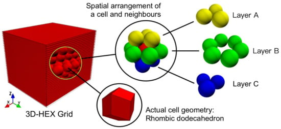
Figure 1.
Schematic view of 3D-HEX grid and spatial arrangement of a cell and its neighbors.
To describe the grain morphology, we use the sphericity degree as a shape factor [27,28,29]. It is the ratio of the diameter of a sphere with the same volume as the grain to the diameter of a sphere with the same surface area as the grain. The sphericity degree varies between 0 and 1, where 0 corresponds to a perfect sphere and 1 signifies a chain-like shape. The sphericity degree reflects how closely the grain resembles a spherical shape and can be used to quantify the effects of grain growth and deformation on microstructure evolution.
Based on this idea, we propose a new model to calculate the grain shape factor in 3D-HEX using the surface area and volume of an actual grain. The steps are: (1) Calculate the surface area of the grain by Equation (1). (2) Construct a sphere and a chain with the same volume as the grain. These have the minimum and maximum possible surface areas, respectively. (3) Normalize the surface area of the grain to a value between 0 and 1 by Equation (2). This is the shape factor (A) of the grain. A lower A means a higher sphericity degree and more spherical shape, as in Figure 2a. A higher A means a lower sphericity degree and more chain-like shape, as in Figure 2b.
where Sgrain is the surface area of the actual grain, Ssphere is the surface area of the sphere with the same volume as the grain, and Schain is the surface area of the chain with the same volume as the grain. Ssphere and Schain can be calculated by Equations (3) and (4), respectively. Ngrain_surf is the number of surface cells of the grain (blue spheres in Figure 2c or Figure 2d), Nsphere is the number of surface cells of the sphere (Figure 2a), and Nchain is the number of surface cells of the chain (Figure 2b). Scell is the area of a cell’s great circle on its circumscribed sphere. This value can be ignored because it cancels out. Therefore, Equation (2) turns into:
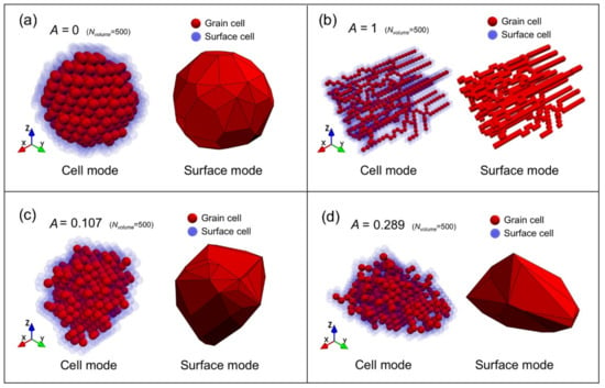
Figure 2.
Schematic view of (a) volume-equivalent-sphere, (b) volume-equivalent-chain, and (c,d) two grains with volume of 500.
Note that Equations (1)–(4) are used to derive Equation (5) and that Equation (5) should be used directly instead of calculating it from Equation (1). To calculate Nsphere and Nchain in Equation (5), we need to build models of spheres and chains with the same volume as the grain. The volume is Nvolume, which is the number of cells in the grain. We use a step-by-step growth CA method to add cells to the models. For spheres, we choose the cell that minimizes the surface-area increase. For chains, we choose the cell that maximizes it. This way, we can simulate different grain morphologies with different sphericity degrees. The spheres have a high sphericity degree close to 0, while the chains have a low sphericity degree close to 1. The step-by-step growth CA method allows us to control the size and shape of the grains by adjusting the number and location of the cells added. Then, we count Nsphere and Nchain for each model with different Nvolume values (from 1 to 5000). We fit curves for Nsphere and Nchain as functions of Nvolume by least squares and plot them in Figure 3 with the actual values [30].
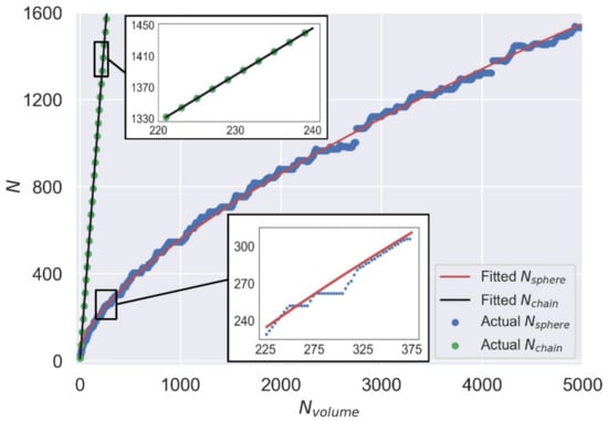
Figure 3.
Relationships between surface cell number of volume-equivalent-sphere (red curve and blue dots), volume-equivalent-chain (black curve and green dots), and their corresponding grain volume number.
Figure 3 shows that Nchain and Nvolume have a linear relationship in the chain model, implying that each Nvolume adds six units of surface area. In contrast, Nsphere has a more complex relationship with Nvolume in the sphere model, which can be approximated by Equation (7). To assess the quality of this approximation, we use residual analysis (Equation (8)), where R is the average residual, and a good fit is expected to have R < 0.05 [31]. Ni and are the actual and fitted values of Nsphere when Nvolume = i. However, Equation (7) has a high R value of 0.115, indicating a poor fit, especially when Nvolume < 200 (see red dotted curves in Figure 4a,b).
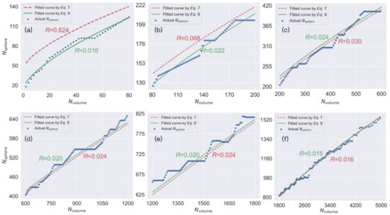
Figure 4.
Comparison of fitting effect between Equation (9) and Equation (7) with volume number within a range of (a) 1~79, (b) 80~199, (c) 200~599, (d) 600~1199, (e) 1200~1799, and (f) 1800~5000.
Piecewise fitting can improve the fitting accuracy by dividing the data into segments and using different functions for each segment that best fit the data within that segment [30]. In this way, the piecewise function can capture nonlinear patterns and discontinuities in the data that a single function might miss. To perform piecewise fitting, we need to specify the number of segments of Nvolume, the functions for each segment, and the breakpoints between segments. Then, we can use various methods to estimate the parameters of each function and minimize the error between the fitted values and the actual values.
Therefore, we use piecewise fitting to improve the accuracy and obtain Equation (9) [30,31]. Figure 4 shows the piecewise fitting results. We recommend using Equation (9) instead of Equation (7) to calculate Nsphere for any given Nvolume. Therefore, with Equations (5) and (9), we can compute the shape factor A of any grain in 3D-HEX using its Nvolume and Ngrain_surf, which are easy and efficient to obtain.
3. Model Validation
Monte Carlo (MC) methods evaluate the validity of a calculation model by comparing the simulated outcomes with the observed or expected outcomes [32]. MC methods use random sampling to generate a large number of possible scenarios based on the input variables and parameters of the model. Then, they analyze the distribution and statistics of the output values to estimate the probabilities, uncertainties, and risks associated with the model. If the simulated outcomes are consistent with the observed or expected outcomes within a certain confidence level, then the model is considered valid. Otherwise, the model may need to be revised or improved. MC methods are widely used in various fields, such as physics, engineering, biology and social sciences. They can handle complex and nonlinear models that are difficult to solve analytically or numerically. They can also incorporate different sources of uncertainty and variability in the input data and parameters. However, MC methods also have some limitations, such as a dependence on random number generators and a difficulty in determining convergence criteria.
We use MC methods to generate 1000 grains in 3D-HEX, including spherical, irregular, and chain grains, to evaluate the validity of A as a shape descriptor. For spherical grains, we choose the cell that minimizes the surface area increase. For chain grains, we choose the cell that maximizes it. For irregular grains, we choose the cell randomly. This way, we can generate different grain morphologies with different sphericity degrees. The step-by-step growth method also allows us to control the size and shape of the grains by adjusting the number and location of the cells added. Figure 5 shows the distribution of A values for these grains.
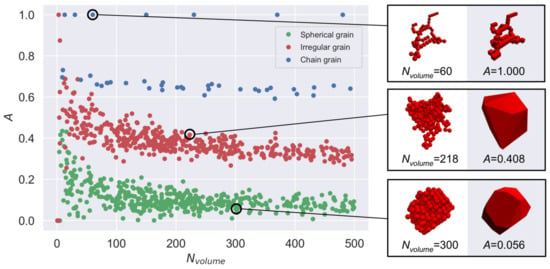
Figure 5.
Distribution of shape factor of spherical grain, irregular grain, and chain grain.
Figure 5 reveals that most spherical grains have A values between 0 and 0.2 (green dots), and most irregular grains have A values between 0.3 and 0.6 (red dots). This agrees with the expected behavior of MC methods, confirming that A can capture the degree of sphericity quantitatively. Note that we use transition rules based on equiaxed grain formation rather than dendrite formation for MC methods in this paper, which results in more low-A grains. However, since chain-like grains have a similar morphology to dendrites and since they always have high A values (blue dots), we can infer that A is also effective for dendrites.
4. Conclusions
The shape factor is a quantitative measure of grain morphology based on the ratio of the surface area of the grain to its volume-equivalent-sphere and volume-equivalent-chain. It indicates how the shape of a grain or phase affects its mechanical properties, such as stiffness, deformation, and fracture. For example, spherical grains tend to have a higher stiffness and lower ductility than chain-like grains. Therefore, controlling the shape factor of grains can be an effective way to optimize the performance of materials.
We propose a novel model to calculate the shape factor of grains in 3D-HEX CA, which overcomes disadvantages, such as complex algorithms and a long computation time. The basic idea of this model is to use the ratio of the actual surface area of a grain to the minimum surface area of a sphere with the same volume as the shape factor for spheres and to use the ratio of the actual surface area of a grain to the maximum surface area of a chain with the same volume as the shape factor for chains. The smaller this ratio is for spheres or the larger it is for chains, the more spherical or chain-like, respectively, the grain is. This model has the following advantages: (1) it is accurate and effective, especially for simulating microstructure evolution; (2) it is normalized, so it can compare grains with different volumes; and (3) it is based on the grain surface area, so it can be integrated with other models that involve grain boundary, grain surface energy, grain classification, etc.
Author Contributions
Conceptualization, L.B. and J.S. methodology, L.B.; software, L.B. and J.S.; validation, L.B. and J.S.; formal analysis, L.B.; investigation, L.B. and J.S.; resources, L.B.; data curation, L.B.; writing—original draft preparation, L.B.; writing—review and editing, L.B. and J.S.; visualization, J.S.; supervision, L.B.; project administration, L.B.; All authors have read and agreed to the published version of the manuscript.
Funding
This research received no external funding.
Institutional Review Board Statement
Not applicable.
Informed Consent Statement
Not applicable.
Data Availability Statement
Data sharing not applicable.
Conflicts of Interest
The authors declare no conflict of interest.
References
- Hashemi, S.; Kalidindi, S.R. A Machine Learning Framework for the Temporal Evolution of Microstructure during Static Recrystallization of Polycrystalline Materials Simulated by Cellular Automaton. Comput. Mater. Sci. 2021, 188, 110132. [Google Scholar] [CrossRef]
- Park, J.; Rout, M.; Min, K.-M.; Chen, S.-F.; Lee, M.-G. A Fully Coupled Crystal Plasticity-Cellular Automata Model for Predicting Thermomechanical Response with Dynamic Recrystallization in AISI 304LN Stainless Steel. Mech. Mater. 2022, 167, 104248. [Google Scholar] [CrossRef]
- Mohebbi, M.S.; Ploshikhin, V. Implementation of Nucleation in Cellular Automaton Simulation of Microstructural Evolution during Additive Manufacturing of Al Alloys. Addit. Manuf. 2020, 36, 101726. [Google Scholar] [CrossRef]
- Ogawa, J.; Natsume, Y. Three-Dimensional Large-Scale Grain Growth Simulation Using a Cellular Automaton Model. Comput. Mater. Sci. 2021, 199, 110729. [Google Scholar] [CrossRef]
- Gu, C.; Moodispaw, M.P.; Luo, A.A. Cellular Automaton Simulation and Experimental Validation of Eutectic Transformation during Solidification of Al-Si Alloys. Npj Comput. Mater. 2022, 8, 134. [Google Scholar] [CrossRef]
- Liu, S.; Hong, K.; Shin, Y.C. A Novel 3D Cellular Automata-Phase Field Model for Computationally Efficient Dendrite Evolution during Bulk Solidification. Comput. Mater. Sci. 2021, 192, 110405. [Google Scholar] [CrossRef]
- Nutaro, J.; Stump, B.; Shukla, P. Discrete Event Cellular Automata: A New Approach to Cellular Automata for Computational Material Science. Comput. Mater. Sci. 2023, 219, 111990. [Google Scholar] [CrossRef]
- Gu, C.; Ridgeway, C.D.; Cinkilic, E.; Lu, Y.; Luo, A.A. Predicting Gas and Shrinkage Porosity in Solidification Microstructure: A Coupled Three-Dimensional Cellular Automaton Model. J. Mater. Sci. Technol. 2020, 49, 91–105. [Google Scholar] [CrossRef]
- Liu, S.; Jiang, Y.; Lu, R.; Cheng, X.; Li, J.; Chen, Y.; Tian, G. Cellular Automata Simulation of Grain Growth of Powder Metallurgy Nickel-Based Superalloy. arXiv 2021, arXiv:2106.04888. [Google Scholar] [CrossRef]
- El Amri, N.; El Amri, A.; El Bouayadi, R.; El Hassouani, Y.; Bouachrine, M.; Zorkani, I. Modeling Phase Change Materials Using Cellular Automata. In Advances in Intelligent Systems and Computing; Benyounes, H., Bouchaala, F.M., Eds.; Springer: Cham, Switzerland, 2020; Volume 1076, pp. 161–170. [Google Scholar] [CrossRef]
- Chen, F.; Tian, X.; Wu, G.; Zhu, H.; Ou, H.; Cui, Z. Coupled Quantitative Modeling of Microstructural Evolution and Plastic Flow during Continuous Dynamic Recrystallization. Int. J. Plast. 2022, 156, 103372. [Google Scholar] [CrossRef]
- Bays, C. Cellular Automata in Triangular, Pentagonal, and Hexagonal Tessellations. In Cellular Automata: A Volume in the Encyclopedia of Complexity and Systems Science, 2nd ed.; Adamatzky, A., Ed.; Encyclopedia of Complexity and Systems Science Series; Springer: New York, NY, USA, 2018; pp. 1–10. ISBN 978-1-4939-8700-9. [Google Scholar]
- Fuyong, S.; Wenli, L.; Zhi, W. Three-Dimensional Cellular Automaton Simulation of Austenite Grain Growth of Fe-1C-1.5Cr Alloy Steel. J. Mater. Res. Technol. 2020, 9, 180–187. [Google Scholar] [CrossRef]
- Rolchigo, M.; Plotkowski, A.; Belak, J. Sensitivity of Cellular Automata Grain Structure Predictions for High Solidification Rates. Comput. Mater. Sci. 2021, 196, 110498. [Google Scholar] [CrossRef]
- Ren, Z.; Pu, Z.; Liu, D.-R. Prediction of Grain-Size Transition during Solidification of Hypoeutectic Al-Si Alloys by an Improved Three-Dimensional Sharp-Interface Model. Comput. Mater. Sci. 2022, 203, 111131. [Google Scholar] [CrossRef]
- Shterenlikht, A.; Margetts, L. Three-Dimensional Cellular Automata Modelling of Cleavage Propagation across Crystal Boundaries in Polycrystalline Microstructures. Proc. R. Soc. A Math. Phys. Eng. Sci. 2015, 471, 20150039. [Google Scholar] [CrossRef]
- Gu, C.; Lu, Y.; Ridgeway, C.D.; Cinkilic, E.; Luo, A.A. Three-Dimensional Cellular Automaton Simulation of Coupled Hydrogen Porosity and Microstructure during Solidification of Ternary Aluminum Alloys. Sci. Rep. 2019, 9, 13099. [Google Scholar] [CrossRef]
- Li, X.; Yang, X.; Xue, C.; Wang, S.; Zhang, Y.; Wang, B.; Wang, J.; Lee, P.D. Predicting Hydrogen Microporosity in Long Solidification Range Ternary Al-Cu-Li Alloys by Coupling CALPHAD and Cellular Automata Model. Comput. Mater. Sci. 2023, 222, 112120. [Google Scholar] [CrossRef]
- Liu, R.; Li, K.; Zhou, G.; Tang, W.; Shen, Y.; Tang, D.; Li, D. Simulation of Strain Induced Abnormal Grain Growth in Aluminum Alloy by Coupling Crystal Plasticity and Phase Field Methods. Trans. Nonferrous Met. Soc. China 2022, 32, 3873–3886. [Google Scholar] [CrossRef]
- Nabavizadeh, S.A.; Eshraghi, M.; Felicelli, S.D. Three-Dimensional Phase Field Modeling of Columnar to Equiaxed Transition in Directional Solidification of Inconel 718 Alloy. J. Cryst. Growth 2020, 549, 125879. [Google Scholar] [CrossRef]
- Gu, C.; Ridgeway, C.D.; Moodispaw, M.P.; Luo, A.A. Multi-Component Numerical Simulation and Experimental Study of Dendritic Growth during Solidification Processing. J. Mater. Process. Technol. 2020, 286, 116829. [Google Scholar] [CrossRef]
- Wang, Y.; Li, Q.; Zhang, X.; Liu, W. A Continuous-Discontinuous Cellular Automaton Method for Cracks Growth and Coalescence in Brittle Material. Acta Mech. Sin. 2014, 30, 1239–1255. [Google Scholar] [CrossRef]
- Lee, J.; Kim, H.; Lee, C.; Kim, N. A Fully Coupled Crystal Plasticity-Cellular Automata Model for Dynamic Recrystallization of Metallic Materials. Int. J. Plast. 2022, 149, 103127. [Google Scholar] [CrossRef]
- Chen, L.; Liu, F.; Jin, S.; Wang, Y.; Fu, P.; Yang, G. Cellular Automata Simulation of Grain Growth of Powder Metallurgy Ni-Based FGH98 Superalloys during Solution Treatment. J. Iron Steel Res. Int. 2023, 30, 1–11. [Google Scholar]
- Du, L.; Zhang, P.; Wang, L.; Zheng, B.; Du, H. Phase Field Simulation on the Effect of Micropore Morphology on Grain Growth in Porous Ceramics. Comput. Mater. Sci. 2017, 131, 196–201. [Google Scholar] [CrossRef]
- Cagigas-Muñiz, D.; Diaz-del-Rio, F.; Sevillano-Ramos, J.L.; Guisado-Lizar, J.-L. Efficient Simulation Execution of Cellular Automata on GPU. Simul. Model. Pract. Theory 2022, 118, 102519. [Google Scholar] [CrossRef]
- Ye, Z.; Hilden, M.M.; Yahyaei, M. A 3D Cellular Automata Ore Stockpile Model—Part 1: Simulation of Size Segregation. Miner. Eng. 2022, 187, 107816. [Google Scholar] [CrossRef]
- Rorato, R.; Arroyo, M.; Andò, E.; Gens, A. Sphericity Measures of Sand Grains. Eng. Geol. 2019, 254, 43–53. [Google Scholar] [CrossRef]
- Cruz-Matías, I.; Ayala, D.; Hiller, D.; Gutsch, S.; Zacharias, M.; Estradé, S.; Peiró, F. Sphericity and Roundness Computation for Particles Using the Extreme Vertices Model. J. Comput. Sci. 2019, 30, 28–40. [Google Scholar] [CrossRef]
- Ferreira Schon, A.; Apoena Castro, N.; dos Santos Barros, A.; Eduardo Spinelli, J.; Garcia, A.; Cheung, N.; Luiz Silva, B. Multiple Linear Regression Approach to Predict Tensile Properties of Sn-Ag-Cu (SAC) Alloys. Mater. Lett. 2021, 304, 130587. [Google Scholar] [CrossRef]
- Linear Regression Using R: An Introduction to Data Modeling. Available online: https://open.umn.edu/opentextbooks/textbooks/399 (accessed on 12 March 2023).
- Crowder, S.; Delker, C.; Forrest, E.; Martin, N. Monte Carlo Methods for the Propagation of Uncertainties. In Introduction to Statistics in Metrology; Crowder, S., Delker, C., Forrest, E., Martin, N., Eds.; Springer International Publishing: Cham, Switzerland, 2020; pp. 153–180. ISBN 978-3-030-53329-8. [Google Scholar]
Disclaimer/Publisher’s Note: The statements, opinions and data contained in all publications are solely those of the individual author(s) and contributor(s) and not of MDPI and/or the editor(s). MDPI and/or the editor(s) disclaim responsibility for any injury to people or property resulting from any ideas, methods, instructions or products referred to in the content. |
© 2023 by the authors. Licensee MDPI, Basel, Switzerland. This article is an open access article distributed under the terms and conditions of the Creative Commons Attribution (CC BY) license (https://creativecommons.org/licenses/by/4.0/).