Abstract
Compressive strength is a well-known measurement to evaluate the endurance of a given concrete mixture to stress factors, such as compressive loads. A suggested approach to assess compressive strength of concrete is to assume that it follows a probability model from which its reliability is calculated. In reliability analysis, a probability distribution’s reliability function is used to calculate the probability of a specimen surviving to a certain threshold without damage. To approximate the reliability of a subject of interest, one must estimate the corresponding parameters of the probability model. Researchers typically formulate an optimization problem, which is often nonlinear, based on the maximum likelihood theory to obtain estimates for the targeted parameters and then estimate the reliability. Nevertheless, there are additional nonlinear optimization problems in practice from which different estimators for the model parameters are obtained once they are solved numerically. Under normal circumstances, these estimators may perform similarly. However, some might become more robust under irregular situations, such as in the case of data contamination. In this paper, nine frequentist estimators are derived for the parameters of the Laplace Birnbaum-Saunders distribution and then applied to a simulated data set and a real data set. Afterwards, they are compared numerically via Monte Carlo comparative simulation study. The resulting estimates for the reliability based on these estimators are also assessed in the latter study.
1. Introduction
In reality, concrete is the most widely used construction material in the world. Concrete compressive strength is a measure used in determining the amount of resistance a structural element can offer to deformation. Compressive strength is a widely used measure to access the performance of a given concrete mixture. Considering this approach of concrete is vital due to it is the main measure deciding how well concrete can withstand loads that influence its measure. It precisely tells us whether a particular mix is suitable to meet the necessities of a particular venture. Concrete can astoundingly stand up to compressive loading. This is often why it is reasonable for constructing arches, columns, dams, foundations, and tunnel linings among other structures.
Researchers from different fields of science may attempt to describe phenomena of interest, such as concrete compressive strength, using either mathematical or probabilistic models. For instance, scientists describe the life of an object using a probabilistic model called a lifetime probability distribution. Such practice is common in the scientific community, especially in many science fields that involve reliability and reliability analyses. For example, in material science, the two-parameter Birnbaum-Saunders (BS) lifetime distribution can be used by analysts to model fatigue of materials due to periodic cyclic loading [1,2]. This non-negative lifetime model has unimodal skewed probability density and hazard rate curves. Unimodal hazard rate curves are common in practice; see, for example, Langlands et al. [3]. A non-negative continuous random variable T is said to follow the BS distribution if the corresponding cumulative distribution function (CDF) is given by:
where is the shape parameter, is the scale parameter, and is the CDF of the standard normal distribution. Desmond [4] provided a more general derivation for the BS distribution assuming a biological model which reinforced the physical rationalization for the use of the BS distribution by relaxing the original presumptions of [1,2]. The BS distribution has desirable aspects and a close relationship to the normal distribution. Consequently, at least a couple of hundred papers and a single research monograph have already appeared describing all properties and developments of this distribution; see, for example, the comprehensive review by Balakrishnan and Kundu [5] in this connection. Examples of recent applications of the BS distribution are such as Bourguignon et al. [6], Hassani et al. [7], and Kannan et al. [8], among others. The BS distribution belongs to a generalized family of distributions called the generalized BS distribution [9]. The generalization is obtained by replacing the Gaussian kernel in Equation (1) with kernels of symmetrical distributions such as the Laplace and logistic distributions. Sampling plans from truncated life tests assuming the generalized BS distribution were developed in [10], while the generalized BS distribution was used to analyze air pollutant concentration in [11]. For further details in this connection, see [12]. The Laplace BS (LBS) distribution is a BS distribution based on Laplace kernel. Its properties and some associated estimation methods were studied by Zhu and Balakrishnan [13]. This paper expands upon their work by discussing additional methods to estimate the parameter of the LBS distribution assuming data contamination. A positive random variable is said to follow the LBS distribution if the corresponding CDF, reliability function, and the probability density functions are given by:
and
respectively, such that is a positive shape parameter, while is a positive scale parameter, where:
and
The LBS distribution and other lifetime models are characterized by essential statistical properties such as hazard (failure) rates and reliability. The latter concept represents the probability of a specimen continuing to exist for a certain amount of time without loss. Approximating the aspects of the life of objects of interest (e.g., reliability) is associated with model parameters estimation. Estimating the probability distribution parameters has been of great interest to scientists and has received much attention in the statistical literature. In practice, one can obtain various estimators for the model parameters. Therefore, several researchers conducted comparative Monte Carlo simulation studies to numerically assess the estimators from different statistical and computation perspectives; see, for example, Gupta and Kundu [14], Alkasasbeh and Raqab [15], Mazucheli et al. [16], do Espirito Santo and Mazucheli [17], and Balakrishnan and Alam [18], among other research contributions.
Due to the advancement of human civilization, researchers currently deal with various types and large amounts of data originated from the targeted phenomena. In practice, there is no guarantee that part of the data may be missing or contaminated with unusual information values called outliers or extremes. In both cases, estimation efficiency is negatively impacted since the quality of data became questionable. Under data contamination, the maximum likelihood method is not robust since the deviations caused by existing outliers can negatively affect the likelihood. Data contamination motivated many researchers to propose alternative estimators to those obtained by the maximum likelihood theory for various distributions; see, for example, Lawson et al. [19], Boudt et al. [20], Agostinelli et al. [21], Wang et al. [22], among other papers.
The aim of this paper is twofold. Firstly, the LBS distribution is fitted to a real concrete compressive strength data using nine estimation methods. Secondly, the performances of the resulting estimators from the considered estimation methods; namely, modified moments estimators (MMEs), maximum likelihood estimators (MLEs), the maximum product of spacings estimators (MPSEs), the least-squares estimators (LSEs), the weighted least-squares estimators (WLSEs), the percentile estimators (PCEs), the Cramér-von Mises estimators (CVMEs), the Anderson-Darling estimators (ADEs), and the right-tailed Anderson-Darling estimators (RADEs) are investigated using numerical applications and Monte Carlo simulations. The remaining parts of this article are organized as follows. Section 2 discusses the nine estimation methods of interest. Section 3 illustrates the practical application of the discussed estimators using a simulated data set and a real data set. Section 4 reports the outcomes of extensive Monte Carlo simulation study to compare the performance of each estimator under different settings. Finally, remarks and future research are used to conclude this paper in Section 5.
2. Reliability and Model Parameters Estimation
In this section, eight nonlinear optimization problems are formulated to obtain eight estimators for the and parameters mentioned in the introductory section. The ninth estimators are the MMEs which have closed-form expression [13]. Before establishing the targeted optimization problems, one must discussing some computational considerations to solve them.
2.1. Computational Considerations for the Optimization Process
The first important computational consideration is finding suitable starting values to solve the optimization problems. One of the important and practical aspects of the LBS distribution is that the scale parameter is actually the median of the population. Hence, a reasonable starting value for this parameter is the sample median, i.e., . Regarding the starting value for the shape parameter , one can acquire such value by using the relationship between the LBS distribution and the standard Laplace distribution. In fact, if T follows the LBS distribution with model parameters and , then:
follows the Laplace distribution with the location parameter equals to 0, and the scale parameter equals to . Hence, a starting value for is obtained by determining the sample Z values; say, , based on the observed data and the corresponding sample median , and then finding the mean absolute deviation (MAD) of as a starting value for . That is,
such that
The second computational consideration is the choice of optimization algorithm from which one can obtain the estimators for the LBS distribution. Zhu and Balakrishnan [13] showed that the probability density function of the LBS distribution Equation (4) is continuous, but it is not differentiable at . Consequently, estimators like the MLEs require an optimization method free of derivatives to be obtained, such as the Nelder-Mead algorithm [23]. Note that the latter algorithm is utilized to acquire the remaining estimators to avoid any potential bias in the competitive computations.
2.2. Maximum Likelihood Estimation
Zhu and Balakrishnan [13] have obtained MLEs for and and prove their existence and uniqueness. One approach to obtain such estimators is by solving the following maximization algorithm:
such that are the observed random sample.
2.3. Least-Squares-Based Estimations
Given an observed random sample from the LBS distribution with parameters and . Suppose that are the corresponding observed sample order statistics, and consider the following minimization problem:
Hence, the solutions of the above optimization problem are the LSEs for and given that . However, if , then the solutions of the above minimization problem are the WLSEs of and [24].
2.4. Percentile Estimation
PCEs of and are acquired by fitting a linear model to the theoretical percentiles and the sample percentiles [25,26]. This method requires closed-form cumulative distribution and quantile functions. In the case of the LBS distribution, the cumulative distribution function was given by Equation (2), while the quantile function is defined as:
such that , and is the quantile function of the standard Laplace distribution, i.e., . The PCEs of and are the solutions for the following minimization problem:
where are the observed sample order statistics, and .
2.5. Maximum Product of Spacing Estimation
Another estimators of and that depends on solving a maximization problem are the MPSEs. Recent research indicates that such estimates compete with MLEs in terms of estimation efficiency and asymptotic properties [27,28,29]. Given the observed sample order statistics , then the MPSEs for the model parameters are determined numerically by solving the following maximization problem:
such that
2.6. Goodness-of-Fit Estimations
The remaining three estimators are based on the idea of minimizing goodness-of-fit statistics, i.e., minimizing the difference between the estimated cumulative distribution function and an empirical counterpart. Examples of such statistics are the Cramér-von Mises, the Anderson-Darling, and the right-tailed Anderson-Darling statistics. The CVMEs of and are obtained by evaluating the following minimization problem:
On the other hand, ADEs and RADEs of and are acquired as solutions for the following minimization problems:
and
respectively.
3. Numerical Applications
In this section, a simulated data is analyzed; afterwards, a real data is analyzed for the sake of illustration.
3.1. Simulated Data Analysis
Suppose 15 random observations are generated from the LBS distribution with as shown in Table 1.

Table 1.
Simulated data from LBS distribution with .
The simulated data in Table 1 are obtained according to the following algorithm:
- Generate a random sample from the standard uniform distribution (i.e., .)
- For , obtain the desired simulated random sample from the LBS distribution with model parameters and by using Equation (7), i.e.,such that .
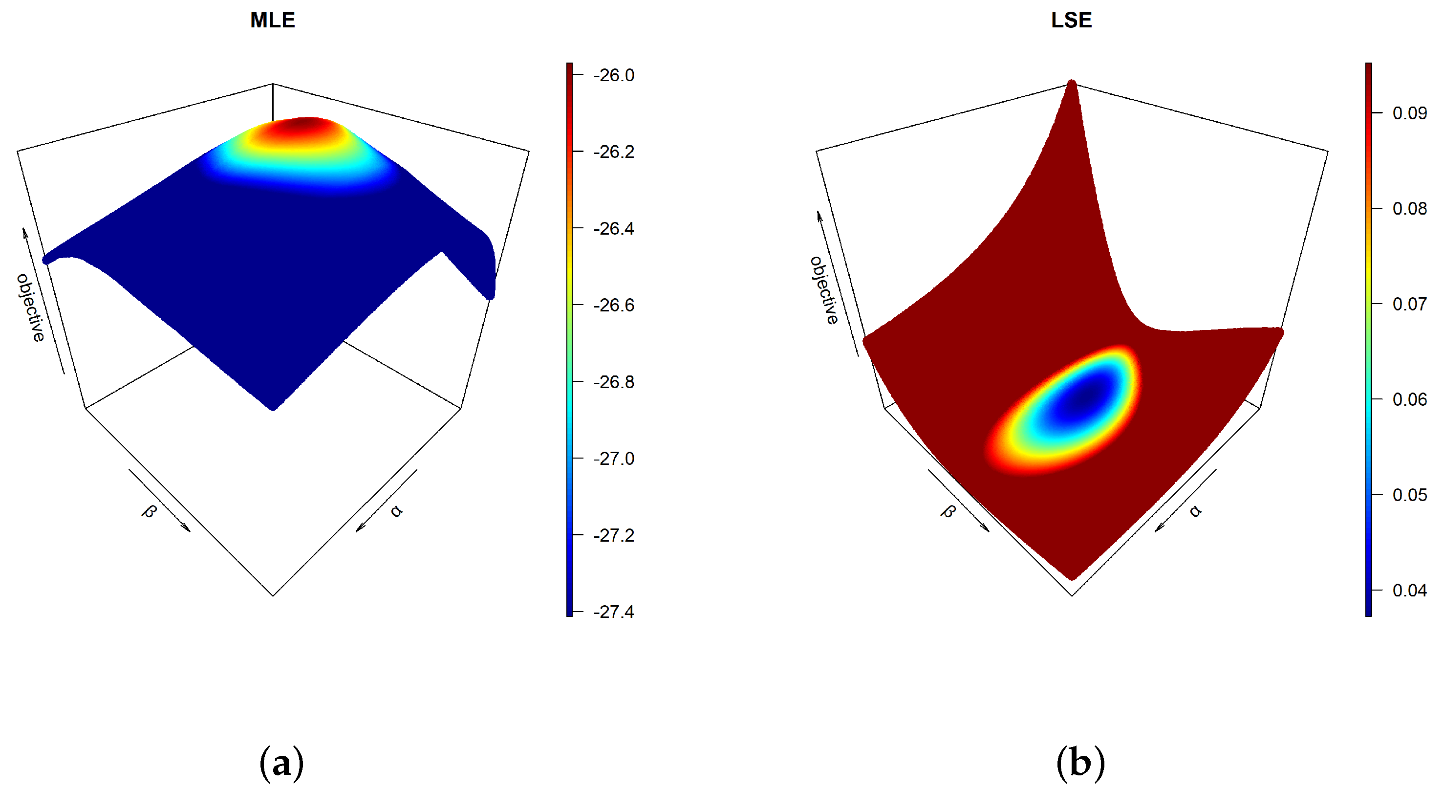
Before obtaining the estimates for and , one must check their existence and uniqueness. Mathematically proving these requirements is beyond the scope of this study; nevertheless, one may prove them using graphical devices. Using extensive Monte Carlo simulations, a three-dimensional (3D) profile plot for each objective function in the preceding section is established, as shown in Figure 1. The 3D charts clearly indicate that there are areas in which global extrema exist and are expected to be unique for each objective function. The MMEs are obtained first for and as shown in [13], and then the remaining estimators are obtained successively as shown in Table 2. The outcomes of the latter table are obtained assuming no contamination in the data, and assuming contamination in the upper 20% order statistics. On the other hand, based on the obtained estimates under both assumptions, Table 3 provides the actual reliability probabilities calculated from the complement of Equation (2) vs. their approximated counterparts using different estimators. Both true and approximated reliability probabilities are evaluated at the sample minimum, the sample three quartiles (, , ), and the sample maximum. From the previous tables, one can easily observe that the PCEs for and provided the farthest approximations for the model parameters and the reliability probabilities. The performances of the remaining estimates are further assessed later.
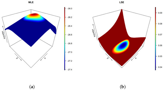
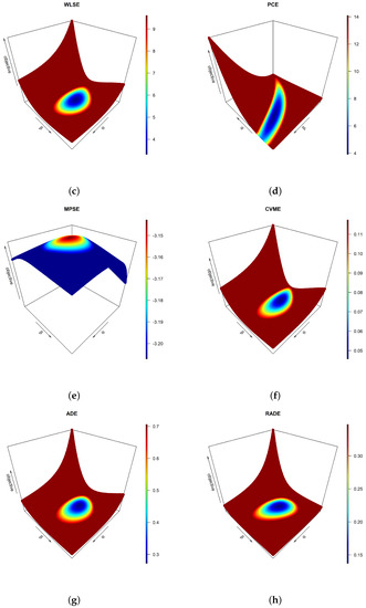
Figure 1.
3D plots of the objective functions based on data in Table 1 for (a) MLE, (b) LSE, (c) WLSE, (d) PCE, (e) MPSE, (f) CVME, (g) ADE and (h) RADE. (cont.)
Table 2.
Estimators of and based on data in Table 1.
Table 3.
True reliability vs. approximated reliability based on estimates in Table 2.
3.2. Real Data Analysis
To illustrate the application of the considered estimation methods in practice, the concrete compressive strength data of [30] is considered for analysis. This data set established from 17 different sources to check the reliability of a suggested strength model. The data gathered concrete comprising cement alongside fly ash, blast furnace slag, and superplasticizer. The data set consisted of a single response variable; namely, the compressive strength of concrete (in MPa), and 8 covariates. Using this data, various estimated models are obtained and compared by the means of Kolmogorov-Smirnov (KS) test. The latter one-sample testing procedure is used to test the null that the distribution function of a given data set is that of the probability distribution of interest. To obtain the KS statistic, one must consider the following steps:
- Obtain the estimates of the parameters and , denoted by and .
- Compute , such that is the observed ith sample order statistics, where . Here, is given by Equation (2).
- Calculate the value of KS statistic as follows:and accordingly calculate the p-value to make a decision about the hypotheses.
Furthermore, since ties exist and the model parameters were estimated, the p-values for the KS statistics were obtained using parametric bootstrapping samples. The steps to obtain the bootstrapping p-value for KS test are as follow:
- For each method, obtain the estimates of the model parameters and ; say, and .
- Use the estimates in the previous step and the algorithm in the preceding section to generate a random sample from the LBS distribution with shape parameter and scale parameter .
- Compute the KS statistics for each bootstrap sample as discussed before, i.e., repeat Steps 2 and 3, B times to obtain .
- Calculate the p-value as follows:where is an indicator function, such that if , and zero otherwise, for and KS is the KS statistic obtained from the original data set.
Finally, it is important to mention that since ties were observed in the data, the MPSEs cannot be acquired directly. When ties exist, one may use a generalization of the maximum product of spacings method to obtain the required estimators; see Murage et al. [31] for additional details. Alongside the estimated parameters and the goodness-of-fit statistics, the reliability probability is calculated at 17 MPa, 28 MPa, and 70 MPa by substituting these values in Equation (3) and replacing the model parameters with the corresponding estimates. In practice, concrete compressive strength can fluctuate between 17 MPa and 28 MPa for residential concrete, while in can be higher as 70 MPa in the case of commercial constructions [32].
Table 4, Table 5, Table 6 and Table 7 respectively summarize the analyses of the considered data set assuming no contamination in the data, 20% of upper data contamination (i.e., the upper 20% of order statistics are multiplied by 5), 20% of lower data contamination (i.e., the lower 20% of order statistics are divided by 5), and 40% two-tailed data contamination which is a mixture of the previous data contamination cases. From the latter tables, one can note the following observations based on the values of the KS test statistics:
Table 4.
Statistical analysis assuming no data contamination.
Table 5.
Statistical analysis assuming 20% of upper data contamination.
Table 6.
Statistical analysis assuming 20% of lower data contamination.
Table 7.
Statistical analysis assuming 40% of two-tailed data contamination.
- When there is no data contamination, both MLEs and MPSEs performed well in terms of goodness-of-fit.
- In the case of upper data contamination, ADEs outperformed both MLEs and MPSEs which took second and third place, respectively.
- On the other hand, both MLEs and MPSEs maintained their performance followed by ADEs in the case of lower data contamination.
- In contrast, WLSEs have perform better than MPSEs and MLEs when two-tailed data contamination exists.
- Overall, MLEs and MPSEs provided the best results in terms of goodness-of-fit, and they both have endured data contamination unlike their counterparts. This is most likely due to the fact that the sample size is large (1000+ units). Furthermore, PCEs and MMEs did not perform well among compared to their counterparts in all considered settings.
- Finally, according to the reliability proportions estimated by MLEs and MPSEs, one can conclude that the sampled specimens of [30] were suitable for residential buildings.
4. Simulation Outcomes
This section presents the outcomes of Monte Carlo simulation experiments based on 1000 random samples from the LBS distribution with different combinations of values for the shape parameter and sample sizes assuming the following scenarios:
- Model 1: A model with no contamination.
- Model 2: A model with 10% of severe upper contamination, i.e., the upper 10% of order statistics are multiplied by 5.
- Model 3: A model with 10% of severe lower contamination, i.e., the lower 10% of order statistics are multiplied by 1/5.
- Model 4: A model with 20% of severe two-tailed contamination, i.e., the upper 10% of order statistics are multiplied by 5, while the lower 10% of order statistics are multiplied by 1/5.
For each scenario, the simulation study assumes , , and , without loss of any generality. To measure estimation efficiency, the simulated bias and simulated root mean-squared-error (RMSE) are calculated as
such that , while () is an estimate of the model parameter () based on simulation repetition i. Furthermore, to measure the goodness-of-fit of the fitted model parameters based on the nine estimators, the average absolute difference between the true and estimated reliability function (), and the maximum absolute difference between the true and estimated reliability function () are determined as
and
respectively, such that , while () is an estimate of the model parameter () based on simulation repetition i.
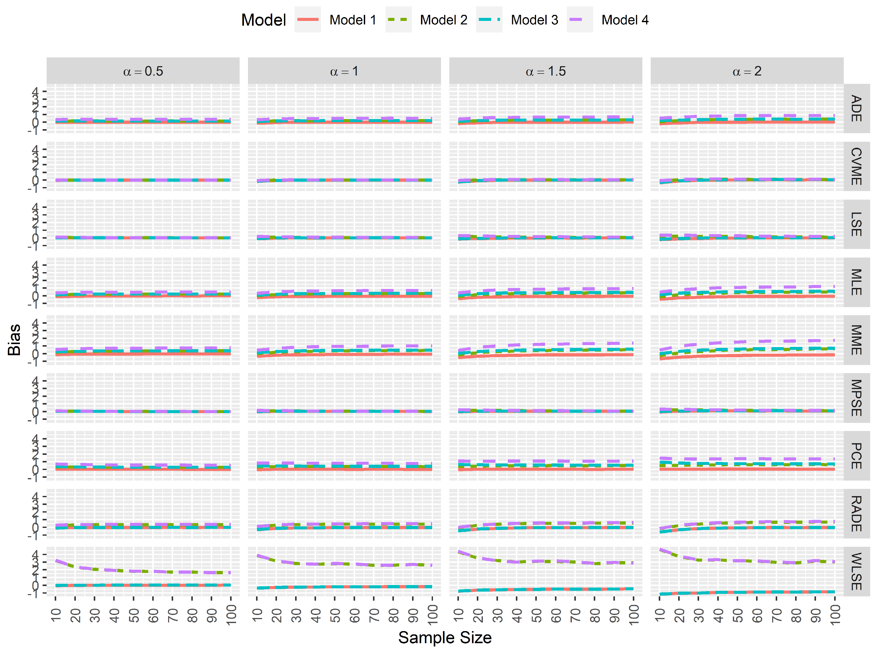
From a statistical perspective, an estimator is computationally consistent when its simulated bias tends to 0 as the sample size increases. Furthermore, when the simulated bias neither increases nor decreases when data contamination exists, then one can conclude that the estimator is computationally robust. Here, Figure 2 and Figure 3 clearly indicate that the most consistent and robust estimators for the model parameters and are the MPSEs and CVMEs regardless of the sample size and the true value of .
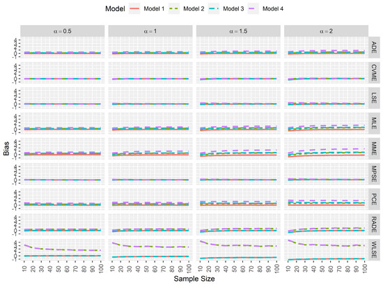
Figure 2.
Simulated biases for the estimators of .
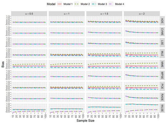
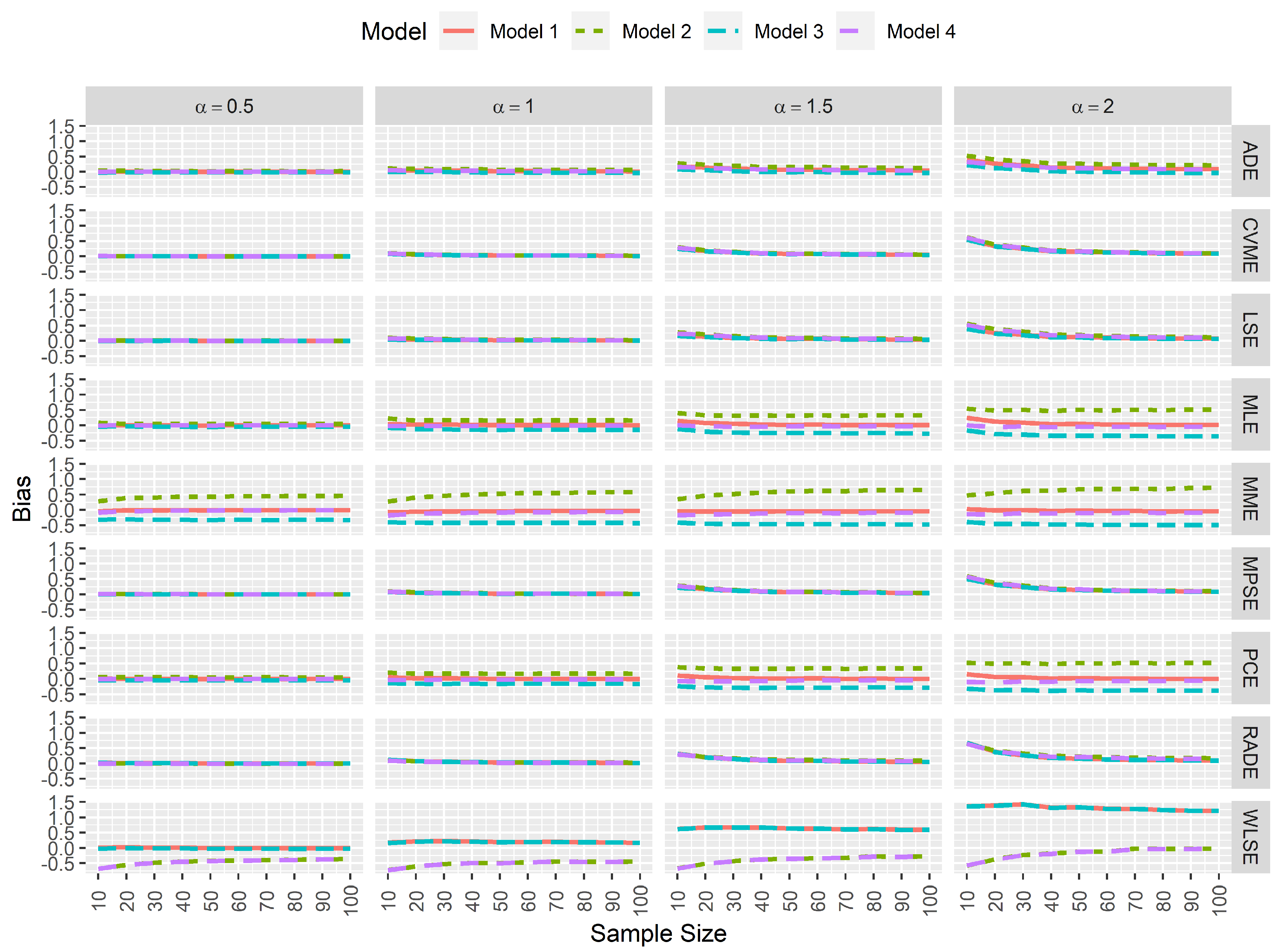
Figure 3.
Simulated biases for the estimators of .
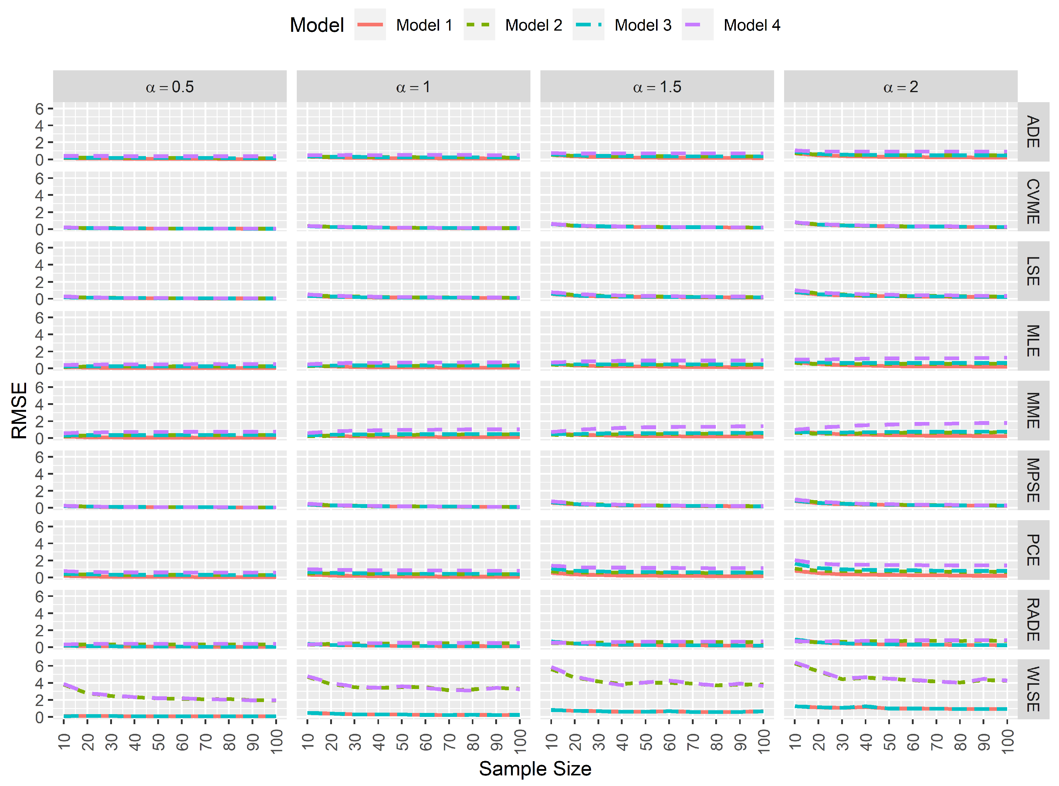
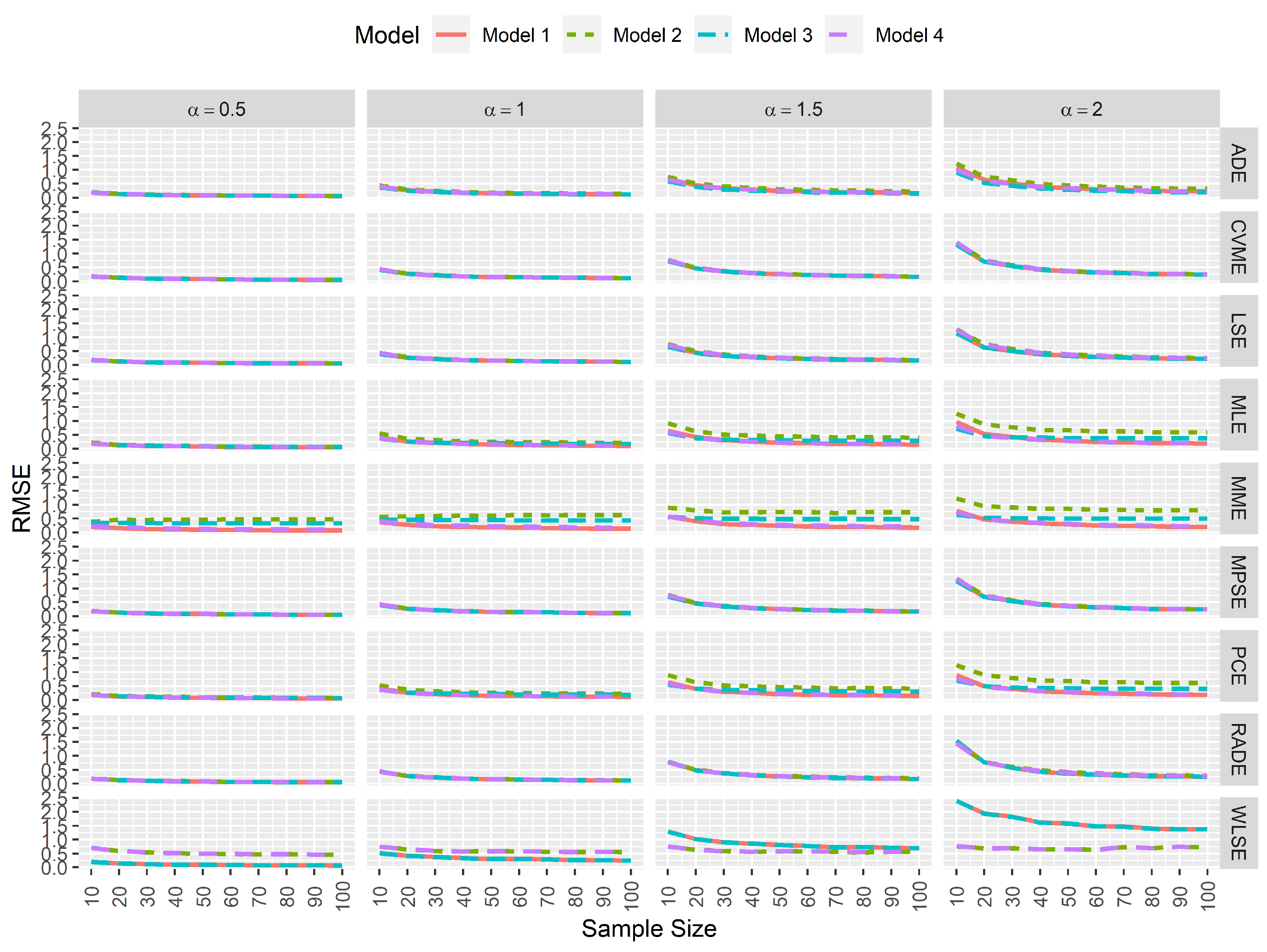
In computational statistics, an estimator is computationally efficient when the simulated RMSE tends to 0 as the sample size increases regardless of the existence of data contamination. Figure 4 and Figure 5 suggest that the MPSEs, CVMEs, and the LSEs of and are the most efficient estimators compared to the other ones regardless of the simulation settings.
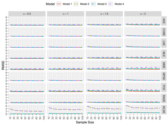
Figure 4.
Simulated RMSEs for the estimators of .
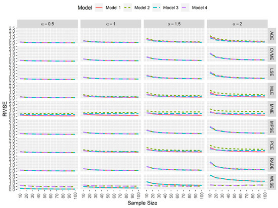
Figure 5.
Simulated RMSEs for the estimators of .
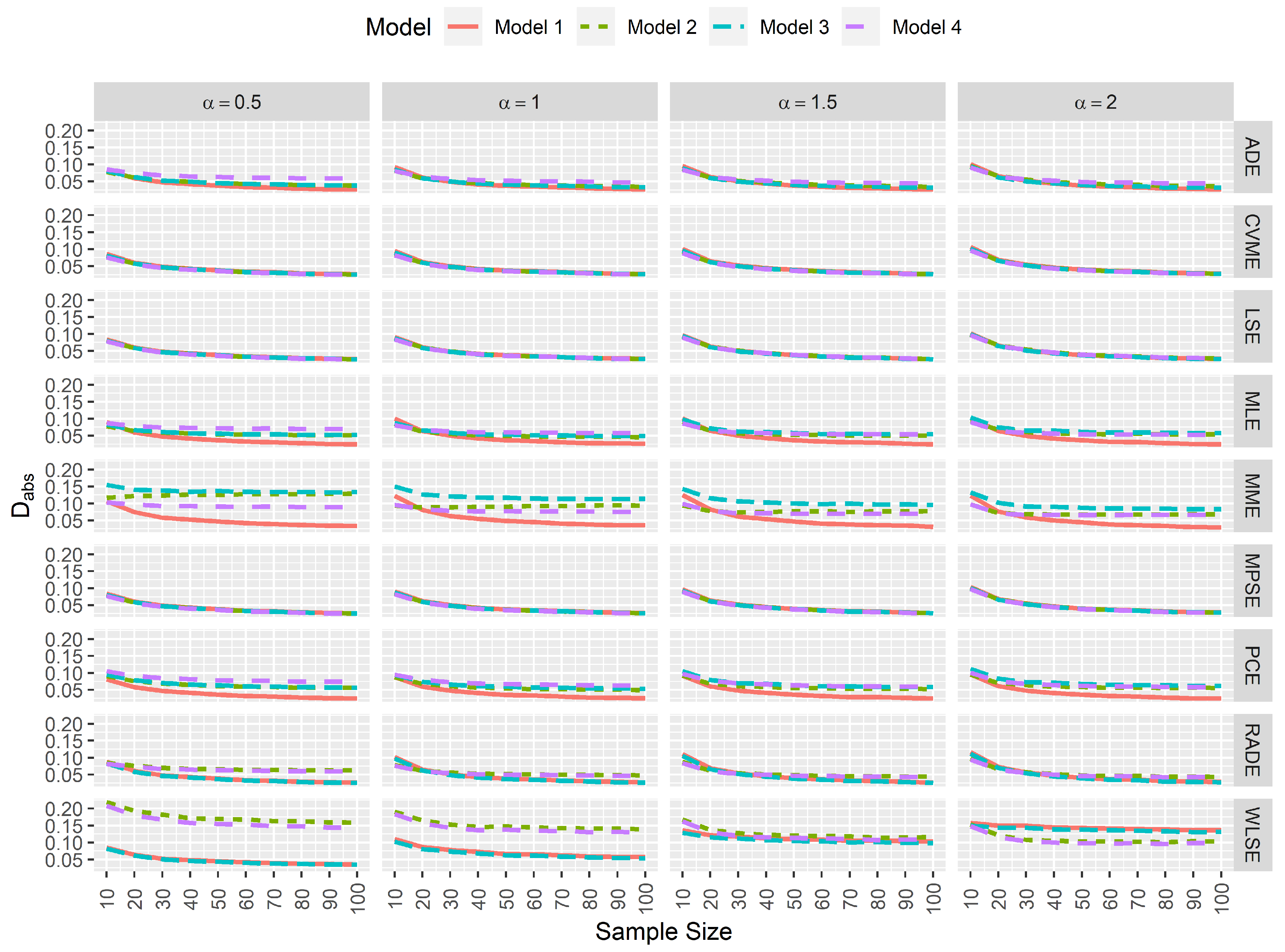
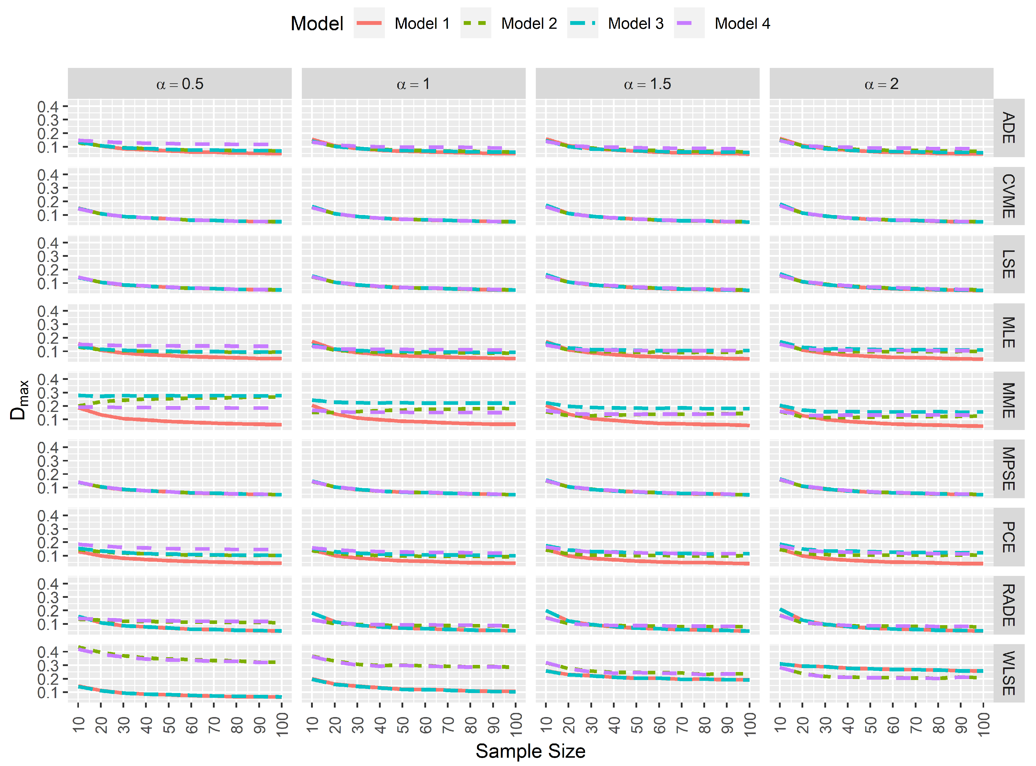
In goodness-of-fit analysis, whenever a pair of estimators yields and that tends to 0 as the sample size increases, and are not negatively affected by data contamination, then this pair of estimates provides the least difference between the true and estimated reliability function. This is very important in practice since the aim is to find the best approximation for the reliability. Figure 6 and Figure 7 again indicate that MPSEs, CVMEs, and the LSEs of and are the estimators that performed well in terms of goodness-of-fit.
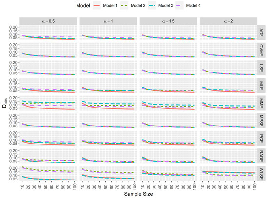
Figure 6.
Simulated average absolute difference between the true and estimated reliability function.
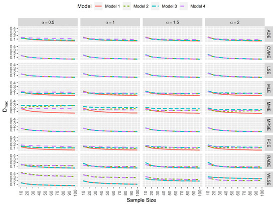
Figure 7.
Simulated maximum absolute difference between the true and estimated reliability function.
5. Conclusions
In this paper, the estimation problem of the parameters and the reliability function of the Laplace Birnbaum-Saunders lifetime distribution is considered. Besides the method of maximum likelihood, eight classical frequentist estimation methods have been discussed for this purpose; namely, modified moments, maximum product of spacings, least-squares, weighted least-squares, percentile, Cramér-von Mises, Anderson-Darling and right-tailed Anderson-Darling estimation methods. Based on the assumption that the invariance property is exist for the different estimation methods, the reliability function is also estimated using the different estimation methods. To compare the performance of the different estimators a Monte Carlo simulation study is conducted. The practical application of the estimators is illustrated by analyzing a simulated data set and one real data set belongs to compressive strength of concrete. Both data analyses and the Monte Carlo simulation study indicated that all methods perform well when there is no contamination in the data. Once there is some contamination in the data, maximum product of spacings, least-squares, and Cramér-von Mises estimates are notably robust compared to the other estimators and the performance of the other method improve as the sample size increases. Data contamination is not the only problem that faces researchers in practice. Data censoring is another practical challenge that needs to be addressed in future research since it negatively impacts estimation efficiency and robustness. Another important research direction is to compare the studied frequentist estimators to Bayesian estimation in terms of performance based on additional real experimental results which are available in literature.
Author Contributions
F.M.A.A. and M.N. contributed equally to this work. Both the authors have read and agreed to the published version of the manuscript.
Funding
This research received no external funding.
Institutional Review Board Statement
Not applicable.
Informed Consent Statement
Not applicable.
Data Availability Statement
No new data were created or analyzed in this study.
Acknowledgments
The authors would like to thank the Editorial Board and two anonymous reviewers for their constructive feedback that improved the final version of the paper.
Conflicts of Interest
The authors declare no conflict of interest.
References
- Birnbaum, Z.; Saunders, S. A new family of life distributions. J. Appl. Probab. 1969, 6, 319–327. [Google Scholar] [CrossRef]
- Birnbaum, Z.W.; Saunders, S.C. Estimation for a Family of Life Distributions with Applications to Fatigue. J. Appl. Probab. 1969, 6, 328–347. [Google Scholar] [CrossRef]
- Langlands, A.O.; Pocock, S.J.; Kerr, G.R.; Gore, S.M. Long–term survival of patients with breast cancer: A study of the curability of the disease. BMJ 1979, 2, 1247–1251. [Google Scholar] [CrossRef] [Green Version]
- Desmond, A. Stochastic models of failure in random environments. Can. J. Stat. 1985, 13, 171–183. [Google Scholar] [CrossRef]
- Balakrishnan, N.; Kundu, D. Birnbaum-Saunders distribution: A review of models, analysis, and applications. Appl. Stoch. Model. Bus. Ind. 2019, 35, 4–49. [Google Scholar] [CrossRef] [Green Version]
- Bourguignon, M.; Ho, L.L.; Fernandes, F.H. Control charts for monitoring the median parameter of Birnbaum-Saunders distribution. Qual. Reliab. Eng. Int. 2020, 36, 1333–1363. [Google Scholar] [CrossRef]
- Hassani, H.; Kalantari, M.; Entezarian, M.R. A new five-parameter Birnbaum–Saunders distribution for modeling bicoid gene expression data. Math. Biosci. 2020, 319, 108275. [Google Scholar] [CrossRef] [PubMed]
- Kannan, G.; Jeyadurga, P.; Balamurali, S. Economic design of repetitive group sampling plan based on truncated life test under Birnbaum–Saunders distribution. Commun. Stat. Simul. Comput. 2020, 1–17. [Google Scholar] [CrossRef]
- Diáz-Garciá, J.A.; Leiva-Sánchez, V. A new family of life distributions based on the elliptically contoured distributions. J. Stat. Plan. Inference 2005, 128, 445–457. [Google Scholar] [CrossRef]
- Balakrishnan, N.; Leiva, V.; López, J. Acceptance Sampling Plans from Truncated Life Tests Based on the Generalized Birnbaum–Saunders Distribution. Commun. Stat. Simul. Comput. 2007, 36, 643–656. [Google Scholar] [CrossRef]
- Leiva, V.; Barros, M.; Paula, G.A.; Sanhueza, A. Generalized Birnbaum-Saunders distributions applied to air pollutant concentration. Environmetrics 2008, 19, 235–249. [Google Scholar] [CrossRef]
- Sanhueza, A.; Leiva, V.; Balakrishnan, N. The Generalized Birnbaum–Saunders Distribution and Its Theory, Methodology, and Application. Commun. Stat. Theory Methods 2008, 37, 645–670. [Google Scholar] [CrossRef]
- Zhu, X.; Balakrishnan, N. Birnbaum-Saunders distribution based on Laplace kernel and some properties and inferential issues. Stat. Probab. Lett. 2015, 101, 1–10. [Google Scholar] [CrossRef]
- Gupta, R.D.; Kundu, D. Generalized exponential distribution: Different method of estimations. J. Stat. Comput. Simul. 2001, 69, 315–337. [Google Scholar] [CrossRef]
- Alkasasbeh, M.R.; Raqab, M.Z. Estimation of the generalized logistic distribution parameters: Comparative study. Stat. Methodol. 2009, 6, 262–279. [Google Scholar] [CrossRef]
- Mazucheli, J.; Louzada, F.; Ghitany, M. Comparison of estimation methods for the parameters of the weighted Lindley distribution. Appl. Math. Comput. 2013, 220, 463–471. [Google Scholar] [CrossRef]
- do Espirito Santo, A.; Mazucheli, J. Comparison of estimation methods for the Marshall–Olkin extended Lindley distribution. J. Stat. Comput. Simul. 2014, 85, 3437–3450. [Google Scholar] [CrossRef] [Green Version]
- Balakrishnan, N.; Alam, F.M.A. Maximum likelihood estimation of the parameters of Student’s t Birnbaum-Saunders distribution: A comparative study. Commun. Stat. Simul. Comput. 2019, 1–30. [Google Scholar] [CrossRef]
- Lawson, C.; Keats, J.; Montgomery, D. Comparison of robust and least-squares regression in computer-generated probability plots. IEEE Trans. Reliab. 1997, 46, 108–115. [Google Scholar] [CrossRef]
- Boudt, K.; Caliskan, D.; Croux, C. Robust explicit estimators of Weibull parameters. Metrika 2009, 73, 187–209. [Google Scholar] [CrossRef] [Green Version]
- Agostinelli, C.; Marazzi, A.; Yohai, V.J. Robust Estimators of the Generalized Log-Gamma Distribution. Technometrics 2014, 56, 92–101. [Google Scholar] [CrossRef]
- Wang, M.; Park, C.; Sun, X. Simple robust parameter estimation for the Birnbaum-Saunders distribution. J. Stat. Distrib. Appl. 2015, 2. [Google Scholar] [CrossRef] [Green Version]
- Nelder, J.A.; Mead, R. A Simplex Method for Function Minimization. Comput. J. 1965, 7, 308–313. [Google Scholar] [CrossRef]
- Swain, J.J.; Venkatraman, S.; Wilson, J.R. Least-squares estimation of distribution functions in johnson’s translation system. J. Stat. Comput. Simul. 1988, 29, 271–297. [Google Scholar] [CrossRef]
- Kao, J.H.K. Computer Methods for Estimating Weibull Parameters in Reliability Studies. IRE Trans. Reliab. Qual. Control. 1958, PGRQC-13, 15–22. [Google Scholar] [CrossRef]
- Kao, J.H.K. A Graphical Estimation of Mixed Weibull Parameters in Life-Testing of Electron Tubes. Technometrics 1959, 1, 389–407. [Google Scholar] [CrossRef]
- Cheng, R.C.H.; Amin, N.A.K. Maximum Product-of-Spacings Estimation with Applications to the Lognormal Distribution; Technical Report 1; Department of Mathematics, University of Wales IST: Cardiff, UK, 1979. [Google Scholar]
- Cheng, R.C.H.; Amin, N.A.K. Estimating Parameters in Continuous Univariate Distributions with a Shifted Origin. J. R. Stat. Soc. Ser. B 1983, 45, 394–403. [Google Scholar] [CrossRef]
- Ranneby, B. The Maximum Spacing Method. An Estimation Method Related to the Maximum Likelihood Method. Scand. J. Stat. 1984, 11, 93–112. [Google Scholar]
- Yeh, I.C. Modeling of strength of high performance concrete using artificial neural networks. Cem. Concr. Res. 1998, 28, 1797–1808. [Google Scholar] [CrossRef]
- Murage, P.; Mungátu, J.; Odero, E. Optimal Threshold Determination for the Maximum Product of Spacing Methodology with Ties for Extreme Events. Open J. Model. Simul. 2019, 7, 149–168. [Google Scholar] [CrossRef] [Green Version]
- NRMCA. Concrete in Practice: What, Why and How? CIP 35—Testing Compressive Strength of Concrete; National Ready Mixed Concrete Association: Silver Spring, MD, USA, 2020. [Google Scholar]

Publisher’s Note: MDPI stays neutral with regard to jurisdictional claims in published maps and institutional affiliations. |
© 2021 by the authors. Licensee MDPI, Basel, Switzerland. This article is an open access article distributed under the terms and conditions of the Creative Commons Attribution (CC BY) license (https://creativecommons.org/licenses/by/4.0/).