A Discrete-Time Homing Problem with Two Optimizers

Abstract

A stochastic difference game is considered in which a player wants to minimize the time spent by a controlled one-dimensional symmetric random walk $\{X_n,n=0,1,\dots \}$ in the continuation region $C:=\{1,2,\dots \}$, and the second player seeks to maximize the survival time in C. The process starts at $X_0=x>0$ and the game ends the first time $X_n\le 0$. An exact expression is derived for the value function, from which the optimal solution is obtained, and particular problems are solved explicitly.

1. Introduction

A deterministic one-dimensional two-player linear-quadratic (nonzero-sum) difference game can be defined as follows (see, for example, [1]):

$$X_{n+1}=a_n{X}_n+b_n{u}_n+c_n{v}_n$$

(1)

for $n\in \{0,1,\dots ,T\}$, where $a_n$, $b_n$ and $c_n$ are deterministic functions, the control $u_n$ (respectively, $v_n$) gives the decision of player 1 (respectively, player 2) at time n. Each player has a general quadratic cost function that he/she tries to minimize.

The difference game can be made stochastic by adding the random variable ${ϵ}_n$ in Equation (1). The random variables ${ϵ}_0,{ϵ}_1,\dots$ are assumed to be independent and identically distributed.

The final time T can be finite or infinite. Reddy and Zaccour [2] considered a class of non-cooperative N-player finite-horizon linear-quadratic dynamic games with linear constraints. Lin [3] studied the Stackelberg strategies in the infinite horizon LQ mean-field stochastic difference game. Liu et al. [4] used an adaptive dynamic programming approach to solve the infinite horizon linear quadratic Stackelberg game problem for unknown stochastic discrete-time systems with multiple decision makers. Ju et al. [5] used dynamic programming to obtain an optimal linear strategy profile for a class of two-player finite-horizon linear-quadratic difference games.

In this paper, we consider the one-dimensional controlled Markov chain $\{X_n,n=0,1,\dots \}$ defined by

$$X_{n+1}=X_n+u_n-v_n+{ϵ}_n\mathrm{for}n=0,1,\dots ,$$

(2)

where ${ϵ}_n=\pm 1$ with probability 1/2 and the random variables ${ϵ}_0,{ϵ}_1,\dots$ are independent, so that $\{X_n,n=0,1,\dots \}$ is a (controlled) symmetric random walk. The chain starts at $X_0=x>0$.

We define the first-passage time

$$T\left(x\right):=inf\{n>0:X_n\le 0\mid X_0=x>0\}.$$

(3)

Our aim is to find the controls $u_n\in \{-1,0\}$ and $v_n\in \{0,1\}$ that minimize the expected value of the cost function

$$J\left(x\right)=\sum _{n=0}^{T\left(x\right)-1}(u_n^2-v_n^2+\lambda ),$$

(4)

where $\lambda$ is a positive constant. This parameter gives the penalty incurred for survival in the continuation region $C:=\{1,2,\dots \}$. It is needed to obtain a well-defined problem. Indeed, if we set $\lambda =0$, then the optimal solution for the first (respectively, second) player is trivially to choose $u_n\equiv 0$ (respectively, $v_n\equiv 1$).

Thus, there are two optimizers. The first one, using $u_n$, would like the Markov chain to hit the origin as soon as possible. Therefore, he/she would like to choose $u_n=-1$, but this generates a cost. On the other hand, the second optimizer wants the Markov chain to remain positive as long as possible. Hence, he/she would prefer to choose $v_n=0$, which however generates no costs. Both optimizers, and especially the second one, must also take into account the value of the constant $\lambda$.

Remark 1.

We could, in theory, assume that the parameter λ is negative. Then, it is mainly the first optimizer who would need to consider the value of λ. See, however, Remark 3.

The main difference between the current paper and the related ones found in the literature is the fact that, in our case, the final time is neither finite or infinite; it is rather a random variable.

The above problem is a particular homing problem, in which a stochastic process is controlled until a certain event occurs. This type of problem was introduced by Whittle ([6] p. 289) for n-dimensional diffusion processes. He also considered the case when we take the risk-sensitivity of the optimizer into account; see [7], as well as [8,9].

The author has written numerous papers on homing problems. In [10,11], these problems where extended to the case of discrete-time Markov chains, whereas in [12] the case of autoregressive processes was treated; see also [13].

In [10,11], the authors considered a problem related to the one defined above, but with only one optimizer. Thus, they treated a stochastic optimal control problem, whereas the problem in the current paper is a stochastic difference game.

To solve our problem, we will use dynamic programming. Let $F\left(x\right)$ be the value function defined by

$$F\left(x\right)=\underset{\begin{array}{c}(u_n,v_n)\\ n=0,\dots ,T\left(x\right)-1\end{array}}{min}E\left[J\left(x\right)\right].$$

(5)

In the next section, the dynamic programming equation satisfied by the function $F\left(x\right)$ will be derived.

2. Dynamic Programming

In theory, we must determine the optimal value of $(u_n,v_n)$ for $n=0,1,\dots ,T\left(x\right)-1$. However, using dynamic programming, the problem is reduced to finding the optimal solution at the initial time $n=0$ only.

Indeed, we can write, making use of Bellman’s principle of optimality, that

$$\begin{array}{ccc}\hfill F\left(x\right)& :=& \underset{\begin{array}{c}(u_n,v_n)\\ n=0,\dots ,T\left(x\right)-1\end{array}}{min}E\left[\sum _{n=0}^{T\left(x\right)-1}(u_n^2-v_n^2+\lambda )\right]\hfill \\ & =& \underset{\begin{array}{c}(u_n,v_n)\\ n=0,\dots ,T\left(x\right)-1\end{array}}{min}\left\{u_0^2-v_0^2+\lambda +E\left[\sum _{n=1}^{T\left(x\right)-1}(u_n^2-v_n^2+\lambda )\right]\right\}\hfill \\ & =& \underset{(u_0,v_0)}{min}\left\{u_0^2-v_0^2+\lambda +E\left[F(x+u_0-v_0+{ϵ}_0)\right]\right\}.\hfill \end{array}$$

(6)

We can now state the following proposition.

Proposition 1.

The value function $F\left(x\right)$ satisfies the dynamic programming equation

$$F\left(x\right)=\underset{(u_0,v_0)}{min}\left\{u_0^2-v_0^2+\lambda +\frac{1}{2}[F(x+u_0-v_0-1)+F(x+u_0-v_0+1)]\right\}.$$

(7)

The equation is subject to the boundary condition

$$F\left(x\right)=0ifx\le 0.$$

(8)

Remark 2.

The usefulness of the value function is that it enables us to determine the optimal controls $u^{*}\left(0\right)$ and $v^{*}\left(0\right)$.

Since $(u_0,v_0)\in \{(-1,0),(-1,1),(0,0),(0,1)\}$, we deduce from Equation (7) that

$$\begin{array}{ccc}\hfill F\left(x\right)& =& min\left\{1+\lambda +\frac{1}{2}\left[F(x-2)+F\left(x\right)\right],\lambda +\frac{1}{2}\left[F(x-3)+F(x-1)\right],\right.\hfill \\ & & \left.\lambda +\frac{1}{2}\left[F(x-1)+F(x+1)\right],-1+\lambda +\frac{1}{2}\left[F(x-2)+F\left(x\right)\right]\right\}.\hfill \end{array}$$

(9)

Now, let $T_0\left(x\right)$ be the random variable that corresponds to $T\left(x\right)$ when $u_n=v_n\equiv 0$. Using the well-known results on the gambler’s ruin problem (see, for instance, ([14] p. 349), we can state that

$$E\left[T_0\left(x\right)\right]=\infty \mathrm{for}\mathrm{any}x>0.$$

(10)

Hence, we would also have

$$E\left[J\right(x\left)\right]=\infty \mathrm{for}\mathrm{any}x>0.$$

(11)

Since the objective is to minimize the expected value of $J\left(x\right)$, we must conclude that the optimal solution is not $(u_0,v_0)=(0,0)$.

Remark 3.

(i) We deduce from what precedes that we cannot choose a value of the parameter λ in the interval $(-\infty ,0)$, otherwise we obtain an infinite expected reward by choosing $u_n=v_n\equiv 0$.

(ii) If $\lambda =0$, then there is no penalty (or reward) for survival in the continuation region $\{1,2,\dots \}$. The optimal solution is obviously $u_n^{*}\equiv 0$. As will be seen below, the optimal value of $v_n$ is 1 for any value of $\lambda \ge 0$.

(iii) If we define

$$T\left(x\right):=inf\{n>0:X_n\le 0\mathrm{or}{X}_n\ge d\mid X_0=x>0\},$$

(12)

then, when $u_n=v_n\equiv 0$, we find that (see, again, ([14] p. 349))

$$E\left[T_0\left(x\right)\right]=x(d-x)\mathrm{for}0\le x\le d,$$

(13)

so that

$$E\left[J\right(x\left)\right]=\lambda x(d-x)\mathrm{for}0\le x\le d.$$

(14)

Therefore, we could take $\lambda <0$ in that case.

(iv) If $P[{ϵ}_n=1]\equiv p$ and $P[{ϵ}_n=-1]\equiv q$ and $T\left(x\right)$ is defined as in (12), then (see ([14] p. 348))

$$E\left[T_0\left(x\right)\right]=\frac{x}{q-p}-\frac{d}{q-p}\frac{1-{(q/p)}^x}{1-{(q/p)}^d}\mathrm{for}0\le x\le d$$

(15)

and

$$\underset{d\to \infty }{lim}E\left[T_0\left(x\right)\right]=\left\{\begin{array}{cc}\infty & \mathrm{if}p\ge 1/2,\hfill \\ \frac{x}{q-p}& \mathrm{if}p<1/2.\hfill \end{array}\right.$$

(16)

Thus, we could consider the case when $\lambda <0$ if $p<1/2$.

Next, notice that $(u_0,v_0)=(-1,0)$ and $(u_0,v_0)=(0,1)$ yield the same expected value of $X_1$. However, the choice $(u_0,v_0)=(-1,0)$ generates a cost of 1, while with $(u_0,v_0)=(0,-1)$ a reward of 1 is obtained. Hence, taking $(u_0,v_0)=(0,1)$ is surely a better decision than choosing $(u_0,v_0)=(-1,0)$. Thus, we must determine whether the optimal solution is $(u_0,v_0)=(-1,1)$ or $(0,1)$.

Proposition 2.

We deduce from what precedes that the second optimizer should choose $v_n\equiv 1$, independently of the value of $u_n$.

Remark 4.

The optimal choice for $u_n$ will depend on the value of the parameter λ, which, as mentioned above, gives the penalty incurred for survival in the continuation region.

It follows from Proposition 2 that Equation (9) can be simplified to

$$F\left(x\right)=min\left\{\lambda +\frac{1}{2}\left[F(x-3)+F(x-1)\right],-1+\lambda +\frac{1}{2}\left[F(x-2)+F\left(x\right)\right]\right\}.$$

(17)

Proposition 3.

The value function $F\left(x\right)$ satisfies the non-linear third-order difference equation

$$\begin{array}{ccc}& & 2F^2\left(x\right)-F\left(x\right)[6\lambda -4+F(x-1)+2F(x-2)+F(x-3)]\hfill \\ & & +F(x-2)\left[F\right(x-1)+F(x-3)+2\lambda ]+2(\lambda -1)\left[F\right(x-1)+F(x-3\left)\right]\hfill \\ & & +4\lambda (\lambda -1)=0\hfill \end{array}$$

(18)

for $x=1,2,\dots$ The boundary condition is

$$F\left(x\right)=0\mathrm{if}x\le 0.$$

(19)

Proof. 

Making use of the formula

$$min\{a,b\}=\frac{a+b-|a-b|}{2},$$

(20)

we deduce from Equation (17) that

$$\begin{array}{ccc}& & 2F\left(x\right)-\left\{-1+2\lambda +\frac{1}{2}[F\left(x\right)+F(x-1)+F(x-2)+F(x-3)]\right\}\hfill \\ & & =-\left|1+\frac{1}{2}[F(x-1)+F(x-3)-F\left(x\right)-F(x-2)]\right|.\hfill \end{array}$$

(21)

By squaring both sides of the above equation and simplifying, we obtain Equation (18). □

Solving a boundary value problem for a non-linear difference equation of order 3 is not easy. Instead of trying to solve Equation (18) directly, we will proceed as in [10].

3. Optimal Choice for ${\mathit{u}}_{\mathit{n}}$

We must determine whether the first optimizer should take $u_0=-1$ or $u_0=0$. The control variable $u_n$ (as well as $v_n$) is actually a function of $X_n$.

Suppose that we set $u_n\left(X_n\right)\equiv -1$. Then, denoting the function $F\left(x\right)$ by $\mathsf{\Phi }\left(x\right)$, Equation (17) implies that

$$\mathsf{\Phi }\left(x\right)=\lambda +\frac{1}{2}\left[\mathsf{\Phi }(x-3)+\mathsf{\Phi }(x-1)\right],$$

(22)

that we rewrite as follows:

$$2\mathsf{\Phi }(y+3)-\mathsf{\Phi }(y+2)-\mathsf{\Phi }\left(y\right)=2\lambda ,$$

(23)

where $y:=x-3$. The equation is valid for $y\in \{-2,-1,\dots \}$ and is subject to the boundary condition

$$\mathsf{\Phi }\left(y\right)=0\mathrm{if}y\le -3.$$

(24)

Making use of the mathematical software program Maple, we find that the solution of Equation (23) that satisfies the boundary conditions $\mathsf{\Phi }(-3)=\mathsf{\Phi }(-4)=\mathsf{\Phi }(-5)=0$ is

$$\mathsf{\Phi }\left(y\right)=\frac{\lambda }{112}\left[210+56y+(i\sqrt{7}-7){\left(\frac{i\sqrt{7}-1}{4}\right)}^y-(i\sqrt{7}+7){\left(\frac{i\sqrt{7}-1}{2}\right)}^{-y}\right]$$

(25)

for $y\ge -3$, so that

$$\mathsf{\Phi }\left(x\right)=\frac{\lambda }{112}\left[42+56x-(i\sqrt{7}+21){\left(\frac{i\sqrt{7}-1}{4}\right)}^x+(i\sqrt{7}-21){\left(\frac{i\sqrt{7}-1}{2}\right)}^{-x}\right]$$

(26)

for $x\ge 0$.

Remark 5.

(i) The function $\mathsf{\Phi }\left(x\right)$ is real, even if it contains the imaginary constant i.

(ii) Because Equation (23) is a third-order linear difference equation, we need three boundary conditions to solve it uniquely. Therefore, we used Equation (24) for $y=-3,-4$ and $-5$.

Next, let us denote the function $F\left(x\right)$ by $\mathsf{\Psi }\left(x\right)$ if we set $u_n\left(X_n\right)\equiv 0$. We then deduce from Equation (17) that the function $\mathsf{\Psi }\left(x\right)$ satisfies the second-order difference equation

$$\mathsf{\Psi }\left(x\right)=-1+\lambda +\frac{1}{2}\left[\mathsf{\Phi }(x-2)+\mathsf{\Phi }\left(x\right)\right].$$

(27)

The unique solution that is such that $\mathsf{\Psi }\left(0\right)=\mathsf{\Psi }(-1)=0$ is

$$\mathsf{\Psi }\left(x\right)=(-1+\lambda )\left[x-\frac{{(-1)}^x}{2}+\frac{1}{2}\right]\mathrm{for}x\ge 0.$$

(28)

Every time the value of $X_n$ changes, the (first) optimizer must make a new decision. It then follows from Equation (17) that we can express the value function $F\left(x\right)$ in terms of $\mathsf{\Phi }\left(x\right)$ and $\mathsf{\Psi }\left(x\right)$ as in the following proposition.

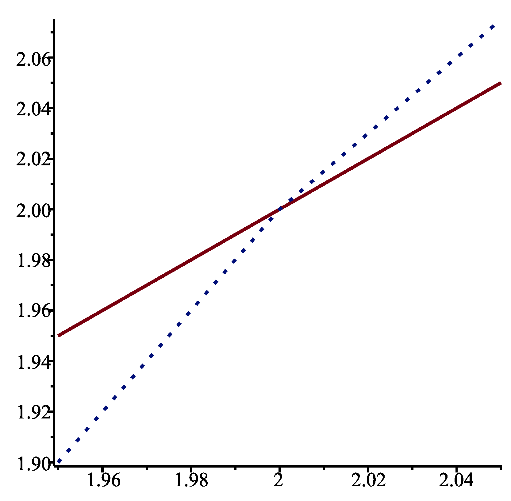
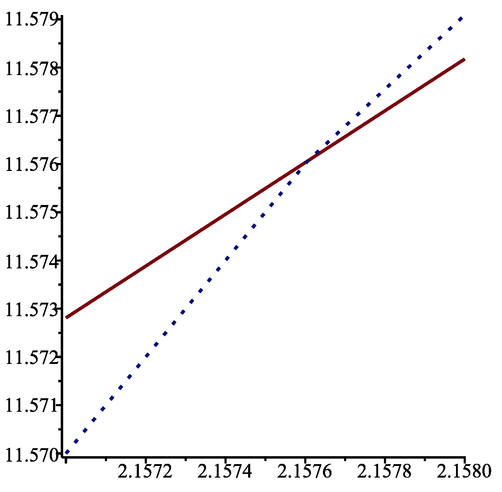
Proposition 4.

The value function $F\left(x\right)$ is given by

$$\begin{array}{ccc}\hfill F\left(x\right)& =& min\{\lambda +\frac{1}{2}\left[min\left\{\mathsf{\Phi }\right(x-3),\mathsf{\Psi }(x-3\left)\right\}+min\left\{\mathsf{\Phi }\right(x-1),\mathsf{\Psi }(x-1\left)\right\}\right],\hfill \\ & & -1+\lambda +\frac{1}{2}\left[min\left\{\mathsf{\Phi }\right(x-2),\mathsf{\Psi }(x-2\left)\right\}+min\left\{\mathsf{\Phi }\right(x),\mathsf{\Psi }(x\left)\right\}\right]\}\hfill \end{array}$$

(29)

for $x=\in \{0,1,\dots \}$.

To determine the value function, and hence the optimal value of $u_0$ ($=u_0\left(x\right)$), we can compare the two expressions

$$G\left(x\right):=\lambda +\frac{1}{2}\left[min\left\{\mathsf{\Phi }\right(x-3),\mathsf{\Psi }(x-3\left)\right\}+min\left\{\mathsf{\Phi }\right(x-1),\mathsf{\Psi }(x-1\left)\right\}\right]$$

(30)

and

$$H\left(x\right):=-1+\lambda +\frac{1}{2}\left[min\left\{\mathsf{\Phi }\right(x-2),\mathsf{\Psi }(x-2\left)\right\}+min\left\{\mathsf{\Phi }\right(x),\mathsf{\Psi }(x\left)\right\}\right].$$

(31)

That is, we can write that

$$F\left(x\right)=min\left\{G\right(x),H(x\left)\right\}.$$

(32)

Remark 6.

We must set $\mathsf{\Psi }(-2)=0$ when we compute the function $G\left(x\right)$ (and $F\left(x\right)$).

In the next section, we will present the results obtained with different values of the parameter $\lambda$ to see the effect of this parameter on the optimal control $u_0^{*}\left(x\right)$.

4. Numerical Examples

Assume first that $\lambda =1/2$. Table 1 gives the value function $F\left(x\right)$, $\mathsf{\Phi }\left(x\right)$, $\mathsf{\Psi }\left(x\right)$, $G\left(x\right)$, $H\left(x\right)$ and the optimal control $u_0^{*}\left(x\right)$ for $x=1,2,\dots ,10$. We see that the optimal control is always $u_0^{*}=0$, which could have been expected because the penalty for survival in the continuation region $C:=\{1,2,\dots \}$ is not large enough to incite the first optimizer to use $u_0=-1$ in order to leave C as rapidly as possible.

Table 1. Functions $F\left(x\right)$, $\mathsf{\Phi }\left(x\right)$, $\mathsf{\Psi }\left(x\right)$, $G\left(x\right)$ and $H\left(x\right)$, and optimal control $u_0^{*}\left(x\right)$ for $x=1,2,\dots ,10$ when $\lambda =1/2$.

x	$\mathit{F}\left(\mathit{x}\right)$	$\mathsf{\Phi }\left(\mathit{x}\right)$	$\mathsf{\Psi }\left(\mathit{x}\right)$	$\mathit{G}\left(\mathit{x}\right)$	$\mathit{H}\left(\mathit{x}\right)$	${\mathit{u}}_0^{*}\left(\mathit{x}\right)$
1	$-1$	$0.5$	$-1$	$0.5$	$-1$	0
2	$-1$	$0.75$	$-1$	0	$-1$	0
3	$-2$	$0.875$	$-2$	0	$-2$	0
4	$-2$	$1.1875$	$-2$	$-1$	$-2$	0
5	$-3$	$1.4687$	$-3$	$-1$	$-3$	0
6	$-3$	$1.6719$	$-3$	$-2$	$-3$	0
7	$-4$	$1.9297$	$-4$	$-2$	$-4$	0
8	$-4$	$2.1992$	$-4$	$-3$	$-4$	0
9	$-5$	$2.4355$	$-5$	$-3$	$-5$	0
10	$-5$	$2.6826$	$-5$	$-4$	$-5$	0

Next, we take $\lambda =1$. This case is rather special, because the function $\mathsf{\Psi }\left(x\right)$ becomes $\mathsf{\Psi }\left(x\right)\equiv 0$. Again, $u_0^{*}\left(x\right)\equiv 0$; see Table 2.

Table 2. Functions $F\left(x\right)$, $\mathsf{\Phi }\left(x\right)$, $\mathsf{\Psi }\left(x\right)$, $G\left(x\right)$ and $H\left(x\right)$, and optimal control $u_0^{*}\left(x\right)$ for $x=1,2,\dots ,10$ when $\lambda =1$.

x	$\mathit{F}\left(\mathit{x}\right)$	$\mathsf{\Phi }\left(\mathit{x}\right)$	$\mathsf{\Psi }\left(\mathit{x}\right)$	$\mathit{G}\left(\mathit{x}\right)$	$\mathit{H}\left(\mathit{x}\right)$	${\mathit{u}}_0^{*}\left(\mathit{x}\right)$
1	0	1	0	1	0	0
2	0	$1.5$	0	1	0	0
3	0	$1.75$	0	1	0	0
4	0	$2.375$	0	1	0	0
5	0	$2.937$	0	1	0	0
6	0	$3.344$	0	1	0	0
7	0	$3.859$	0	1	0	0
8	0	$4.398$	0	1	0	0
9	0	$4.871$	0	1	0	0
10	0	$5.365$	0	1	0	0

In Table 3, $\lambda =2$. This time, $u_0^{*}\left(x\right)$ is not a constant: $u_0^{*}\left(1\right)=-1$ or 0 and then $u_0^{*}\left(x\right)=-1$ for x odd and $u_0^{*}\left(x\right)=0$ for x even.

Table 3. Functions $F\left(x\right)$, $\mathsf{\Phi }\left(x\right)$, $\mathsf{\Psi }\left(x\right)$, $G\left(x\right)$ and $H\left(x\right)$, and optimal control $u_0^{*}\left(x\right)$ for $x=1,2,\dots ,10$ when $\lambda =2$.

x	$\mathit{F}\left(\mathit{x}\right)$	$\mathsf{\Phi }\left(\mathit{x}\right)$	$\mathsf{\Psi }\left(\mathit{x}\right)$	$\mathit{G}\left(\mathit{x}\right)$	$\mathit{H}\left(\mathit{x}\right)$	${\mathit{u}}_0^{*}\left(\mathit{x}\right)$
1	2	2	2	2	2	$-1$ or 0
2	2	3	2	3	2	0
3	3	$3.5$	4	3	$3.75$	$-1$
4	4	$4.75$	4	$4.75$	4	0
5	5	$5.875$	6	5	$5.687$	$-1$
6	6	$6.687$	6	$6.687$	6	0
7	7	$7.719$	8	7	$7.797$	$-1$
8	8	$8.797$	8	$8.797$	8	0
9	9	$9.742$	10	9	$9.730$	$-1$
10	10	$10.730$	10	$10.730$	10	0

Finally, $\lambda =10$ in Table 4 and the optimal control is $u_0^{*}\left(x\right)\equiv -1$, which is not surprising because the constant $\lambda$ is large.

Table 4. Functions $F\left(x\right)$, $\mathsf{\Phi }\left(x\right)$, $\mathsf{\Psi }\left(x\right)$, $G\left(x\right)$ and $H\left(x\right)$, and optimal control $u_0^{*}\left(x\right)$ for $x=1,2,\dots ,10$ when $\lambda =10$.

x	$\mathit{F}\left(\mathit{x}\right)$	$\mathsf{\Phi }\left(\mathit{x}\right)$	$\mathsf{\Psi }\left(\mathit{x}\right)$	$\mathit{G}\left(\mathit{x}\right)$	$\mathit{H}\left(\mathit{x}\right)$	${\mathit{u}}_0^{*}\left(\mathit{x}\right)$
1	10	10	18	10	14	$-1$
2	15	15	18	15	$16.5$	$-1$
3	$17.5$	$17.5$	36	$17.5$	$22.75$	$-1$
4	$23.75$	$23.75$	36	$23.75$	$28.375$	$-1$
5	$29.375$	$29.375$	54	$29.375$	$32.437$	$-1$
6	$33.437$	$33.437$	54	$33.437$	$37.594$	$-1$
7	$38.594$	$38.594$	72	$38.594$	$42.984$	$-1$
8	$43.984$	$43.984$	72	$43.984$	$47.711$	$-1$
9	$48.711$	$48.711$	90	$48.711$	$52.652$	$-1$
10	$53.652$	$53.652$	90	$53.652$	$57.818$	$-1$

4.1. Critical Value of $\mathit{\lambda }$

For a fixed x, we can determine the critical value of $\lambda$, that is, the value of $\lambda$ for which $G\left(x\right)=H\left(x\right)$. For instance, we see in Figure 1 that $G\left(1\right)=H\left(1\right)$ when $\lambda =2$. For $\lambda \in (0,2)$, $u_0^{*}\left(1\right)=0$, while $u_0^{*}\left(1\right)=-1$ for $\lambda >2$.

Figure 1. Functions $G\left(1\right)$ (solid line) and $H\left(1\right)$ when $\lambda \in [1.95,2.05]$.

Similarly, $G\left(10\right)$ and $H\left(10\right)$ are both approximately equal to 11.576 when $\lambda \approx 2.1576$; see Figure 2.

Figure 2. Functions $G\left(10\right)$ (solid line) and $H\left(10\right)$ when $\lambda \in [2.157,2.158]$.

4.2. Solution of the Non-Linear Difference Equation

As we mentioned in Section 2, solving the non-linear third-order difference Equation (18), subject to the boundary condition (19), is not an easy task.

We can try to solve Equation (18) recursively. First, making use of the boundary condition (19), we can write that

$$F^2\left(1\right)-F\left(1\right)(3\lambda -2)+2\lambda (\lambda -1)=0.$$

(33)

It follows that

$$\begin{array}{ccc}\hfill F\left(1\right)& =& \frac{1}{2}\left\{(3\lambda -2)\pm \left[\sqrt{{(3\lambda -2)}^2-8\left[\lambda (\lambda -1)\right]}\right]\right\}\hfill \\ & =& \frac{1}{2}\left\{(3\lambda -2)\pm \sqrt{{\lambda }^2-4\lambda +4}\right\}\hfill \\ & =& \frac{1}{2}\left\{(3\lambda -2)\pm |\lambda -2|\right\}.\hfill \end{array}$$

(34)

Because $F\left(1\right)$ can take any real value, it is not obvious to decide which sign to choose in the above equation. If we look at the value of $F\left(1\right)$ in Table 1, Table 2, Table 3 and Table 4, we see that we must in fact choose the minus sign, so that

$$F\left(1\right)=\left\{\begin{array}{cc}2(\lambda -1)& \mathrm{if}\lambda \in (0,2],\hfill \\ \lambda & \mathrm{if}\lambda \ge 2.\hfill \end{array}\right.$$

(35)

Next, we could use the above expression for $F\left(1\right)$ in Equation (18) to determine the value of $F\left(2\right)$, and so forth. It is clear that this technique is tedious. Moreover, without having computed the value of $F\left(x\right)$ as we did above, determining the right sign to choose in the expression for $F\left(x\right)$ that corresponds to the one in Equation (35) is not straightforward.

From what precedes, we may conclude that the method used in this paper to compute the value function explicitly is of interest in itself and could be used to solve boundary value problems for non-linear difference equations, if we can express the function of interest as a particular value function in a stochastic control problem.

To conclude, we will check that the values of the function $F\left(x\right)$ given in Table 1 are such that Equation (18), together with the boundary condition (19), is indeed satisfied for $x=1,2,\dots ,10$ when $\lambda =1/2$.

First, we saw in Equation (35) that $F\left(1\right)=-1$ is a solution of the equation if $\lambda =1/2$. Next, since $F\left(2\right)$ is also equal to $-1$, we must have

$$\begin{array}{ccc}& & 2{(-1)}^2-(-1)[6(1/2)-4+(-1)+0+0]+0+2[(1/2)-1][(-1)+0]\hfill \\ & & +4(1/2)\left[\right(1/2)-1]=0,\hfill \end{array}$$

(36)

which is indeed correct.

The value of $F\left(3\right)$ in Table 1 is $-2$. We must check that

$$\begin{array}{ccc}& & 2{(-2)}^2-(-2)[6(1/2)-4+(-1)+2(-1)+0]+(-1)[(-1)+0+2(1/2)]\hfill \\ & & +2\left[\right(1/2)-1]\left[\right(-1)+0]+4(1/2)\left[\right(1/2)-1]=0.\hfill \end{array}$$

(37)

Again, the result is correct. We can proceed in the same way to check the remaining results. For $x=10$, we obtain that

$$\begin{array}{ccc}& & 2{(-5)}^2-(-5)[6(1/2)-4+(-5)+2(-4)+(-4)]+(-4)[(-5)+(-4)+2(1/2)]\hfill \\ & & +2\left[\right(1/2)-1]\left[\right(-5)+(-4\left)\right]+4(1/2)\left[\right(1/2)-1]=0.\hfill \end{array}$$

(38)

5. Conclusions

Homing problems are generally considered for diffusion processes. The author and Kounta [11] extended these problems to the discrete-time case. In [10], the author improved the results found in [11] by finding an explicit expression for the value function.

In the current paper, a homing problem with two optimizers has been defined and solved explicitly. The problem can be interpreted as a stochastic difference game, as one optimizer is trying to minimize the time spent by the controlled stochastic process in the continuation region C, while the second one seeks to maximize the survival time in C.

In Section 2, the equation satisfied by the value function has been derived. This equation is a non-linear third-order difference equation, which is obviously very difficult to solve explicitly.

The technique that we have used in the paper enables us to obtain an exact expression for the solution of a boundary value problem for a non-linear difference equation. This result is of interest in itself.

For the sake of simplicity, we have considered a symmetric random walk, and it has been assumed that the control variables can take only two values. We could of course generalize the results that have been presented in the paper. However, if there are many possible values for the control variables, obtaining an explicit solution to the homing problem considered can be quite tedious.