Introducing a New Genetic Operator Based on Differential Evolution for the Effective Training of Neural Networks

Abstract

Artificial neural networks are widely established models used to solve a variety of real-world problems in the fields of physics, chemistry, etc. These machine learning models contain a series of parameters that must be appropriately tuned by various optimization techniques in order to effectively address the problems that they face. Genetic algorithms have been used in many cases in the recent literature to train artificial neural networks, and various modifications have been made to enhance this procedure. In this article, the incorporation of a novel genetic operator into genetic algorithms is proposed to effectively train artificial neural networks. The new operator is based on the differential evolution technique, and it is periodically applied to randomly selected chromosomes from the genetic population. Furthermore, to determine a promising range of values for the parameters of the artificial neural network, an additional genetic algorithm is executed before the execution of the basic algorithm. The modified genetic algorithm is used to train neural networks on classification and regression datasets, and the results are reported and compared with those of other methods used to train neural networks.

1. Introduction

Artificial neural networks are machine learning models and have been widely used in recent decades to solve a number of problems [1,2]; they are parametric models commonly defined as $N\left(\overrightarrow{x},\overrightarrow{w}\right)$. The vector $\overrightarrow{x}$ stands for the input pattern, and the vector $\overrightarrow{w}$ represents the associated set of parameters that should be calculated by any optimization method. The calculation is performed by minimizing the so-called training error, expressed as

$$E\left(N\left(\overrightarrow{x},\overrightarrow{w}\right)\right)=\sum _{i=1}^M{\left(N\left({\overrightarrow{x}}_i,\overrightarrow{w}\right)-y_i\right)}^2$$

(1)

The values $\left(\overrightarrow{x_i},y_i\right),i=1,\dots ,M$ form the training set of the problem, where $y_i$ represents the expected outputs for each pattern $\overrightarrow{x_i}$.

Artificial neural networks have been applied to a wide variety of problems in various fields, such as physics [3], astronomy [4], chemistry [5], economics [6], and medicine [7,8]. Equation (1) has been minimized by various methods in the relevant literature. Among them, one can find the backpropagation method [9,10], the RPROP method [11,12,13], quasi-Newton methods [14,15], Simulated Annealing [16], Particle Swarm Optimization (PSO) [17,18], genetic algorithms [19,20], differential evolution [21], Ant Colony Optimization [22], the Gray Wolf Optimizer [23], whale optimization [24], etc. Moreover, Zhang et al. proposed a hybrid algorithm that combines PSO and the backpropagation algorithm for neural network training [25]. Also, many researchers have recently proposed methods that take advantage of parallel processing units in order to speed up the training process [26,27]. Moreover, Kang et al. recently proposed a hybrid method that combines the lattice Boltzmann method [28] and various machine learning methods with the neural networks included in them with good approximation abilities [29]. Furthermore, a series of papers have recently been published that tackle the initialization procedure for the parameters of neural networks. These methods include decision trees [30], the incorporation of Cauchy’s inequality [31], discriminant learning [32], the usage of polynomial bases [33], and the usage of intervals [34]. A systematic review of initialization methods can be found in the work of Narkhede et al. [35].

Additionally, determining the optimal architecture of an artificial neural network can effectively contribute to its training: on the one hand, it will reduce the required training time, and, on the other hand, it will eliminate the problem of overfitting. To tackle this problem, a number of researchers have proposed many methods, such as genetic algorithms [36,37], the application of the PSO method [38], and the application of reinforcement learning [39]. Also, Tsoulos et al. proposed the use of the grammatical evolution technique [40] to construct artificial neural networks [41].

This paper proposes a two-stage technique for the efficient training of artificial neural networks. In the first stage, a genetic algorithm is used to efficiently identify a range of values within which the parameters of the artificial neural network should be optimized. In the second stage, a genetic algorithm is used to optimize these parameters, and it uses a new operator to enhance the results. This new operator is based on the differential evolution technique [42], and it is applied periodically to randomly selected chromosomes of the genetic population. The first stage of the technique is necessary to ensure that the parameters of the artificial neural network are trained within a range of values, which will prevent their overfitting as much as possible. In the second stage, the differential evolution method is selected as the base of the new operator. This method is an evolutionary technique widely used in a series of practical problems, such as community detection [43], structure prediction [44], motor fault diagnosis [45], and clustering techniques [46]. Furthermore, this method is chosen as the basis for the new genetic operator due to the small number of required parameters that must be specified by the user.

The remainder of this article is organized as follows: In Section 2, the proposed method is discussed in detail. In Section 3, the used datasets, as well as the conducted experiment, are discussed. Finally, in Section 4, the conclusions are presented.

2. Method Description

The two phases of the proposed method are analyzed in detail in this section. During the first phase, a genetic algorithm is utilized in order to detect a promising interval of values for the parameters of a neural network. In the second phase, a genetic algorithm that incorporates the suggested operator is applied to minimize the training error of the neural network and the parameters are initialized inside the interval located during the first phase.

2.1. The First Phase of the Proposed Method

In the first phase of the proposed technique, a genetic algorithm is used to identify a range of values for the parameters of the artificial neural network. Genetic algorithms are evolutionary methods, where a series of randomly created candidate solutions, those called chromosomes, are evolved repetitively through a series of steps similar to natural processes such as selection, crossover, and mutation. Genetic algorithms have been used successfully in a series of real-world problems, such as the placement of wind turbines [47], water distribution [48], economics [49], neural network training [50] etc. The neural networks adopted in this manuscript have the following form, as proposed in [41]:

$$N\left(\overrightarrow{x},\overrightarrow{w}\right)=\sum _{i=1}^H{w}_{(d+2)i-(d+1)}\sigma \left(\sum _{j=1}^d{x}_j{w}_{(d+2)i-(d+1)+j}+w_{(d+2)i}\right)$$

(2)

where the value H denotes the total number of processing units in this network and the value d defines the number of inputs for the pattern $\overrightarrow{x}$. Hence, the total number of parameters for this network is $n=(d+2)H$. The function $\sigma \left(x\right)$ is the sigmoid function, defined as follows:

$$\sigma \left(x\right)={\displaystyle \frac{1}{1+\exp (-x)}}$$

(3)

The steps of the algorithm of the first phase are as follows:

• Initialization step.

  (a)

  Set the number of chromosomes $N_c$ and the maximum number of allowed generations $N_g$.

  (b)

  Set the selection rate $p_s$ and the mutation rate $p_m$.

  (c)

  Set the margin factor a, where $a\ge 1$.

  (d)

  Set $k=0$ as the generation counter.

  (e)

  Initialize the chromosomes randomly, $g_i,i=1,\dots ,N_c$. Each chromosome is a vector of parameters for the artificial neural network.

• Fitness calculation step.

  (a)

  For $i=1,\dots ,N_c$ do

  i.

  Create the neural network $N_i\left(\overrightarrow{x},\overrightarrow{g_i}\right)$ for the chromosome $g_i$.

  ii.

  Calculate the associated fitness value $f_i$ as

  $$f_i=\sum _{j=1}^M{\left(N_i\left(\overrightarrow{x_j},\overrightarrow{g_i}\right)-y_j\right)}^2$$

  for the pairs $\left(\overrightarrow{x_j},y_j\right),j=1,\dots ,M$ of the training set.

  (b)

  End For

• Genetic operations step.

  (a)

  Transfer the best $\left(1-p_s\right)\times N_c$ chromosomes of the current generation to the next one. The remaining will be replaced by chromosomes produced in crossover and mutation.

  (b)

  Perform the crossover procedure. During this procedure, for each pair of constructed chromosomes $\left(\tilde{z},\tilde{w}\right)$, two chromosomes will be selected from the current population using tournament selection. The production of the new chromosomes is performed using a process suggested by Kaelo et al. [51].

  (c)

  Perform the mutation procedure. During the mutation procedure, for each element of each chromosome, a random number $r\in [0,1]$ is selected. The corresponding element is altered randomly when $r\le p_m$.

• Termination check step.

  (a)

  Set $k=k+1$.

  (b)

  If $k\le N_g$, then goto the Fitness calculation step.

• Margin creation step.

  (a)

  Obtain the best chromosome $g^{*}$ with the lowest fitness value.

  (b)

  Create the vectors $L^{*}$ and $R^{*}$ as follows:

  $$\begin{array}{ccc}{L}_i^{*}& =& -a\left|g_i^{*}\right|,i=1,\dots ,n\\ R_i^{*}& =& a\left|g_i^{*}\right|,i=1,\dots ,n\end{array}$$

2.2. The Second Phase of the Proposed Method

During the second phase, a second genetic algorithm is used to minimize the training error of the neural network. The parameters of the neural network are initialized inside the vectors $L^{*}$ and $R^{*}$ produced in the previous phase of the algorithm. Also, a novel stochastic genetic operator, which is based on the Differential Evolution approach, is applied periodically to the genetic population. This new stochastic operator is used to improve the performance of randomly selected chromosomes and to speed up the overall genetic algorithm in finding the global minimum. The main steps of the algorithm executed on the second phase are as follows:

• Initialization step.

  (a)

  Set the number of chromosomes $N_c$ and the maximum number of allowed generations $N_g$.

  (b)

  Set the selection rate $p_s\le 1$ and the mutation rate $p_m\le 1$.

  (c)

  Set the crossover probability CR, used in the new genetic operator.

  (d)

  Set the differential weight F that will be used in the novel genetic operator.

  (e)

  Set $N_i$ as the number of generations before the application of the new operator.

  (f)

  Set $N_l$ as the number of chromosomes that will participate in the new operator.

  (g)

  Initialize the $g_i,i=1,\dots ,N_c$ chromosomes inside the vectors $L^{*}$ and $R^{*}$ of the previous phase.

  (h)

  Set $k=0$ the generation counter.

• Fitness calculation step.

  (a)

  For $i=1,\dots ,N_c$ do

  i.

  Produce the corresponding neural network $N_i\left(\overrightarrow{x},\overrightarrow{g_i}\right)$ for the chromosome $g_i$.

  ii.

  Calculate the fitness value $f_i$ as

  $$f_i=\sum _{j=1}^M{\left(N_i\left(\overrightarrow{x_j},\overrightarrow{g_i}\right)-y_j\right)}^2$$

  (b)

  End For

• Application of genetic operators.

  (a)

  Copy the best $\left(1-p_s\right)\times N_c$ chromosomes with the lowest fitness values to the next generation. The remaining will be replaced by chromosomes produced in crossover and mutation.

  (b)

  Apply the same crossover procedure as in the algorithm of the first phase.

  (c)

  Apply the same mutation procedure as in the genetic algorithm of the first phase.

• Application of the novel genetic operator.

  (a)

  If $k\mathrm{mod}{N}_i=0$ then

  i.

  Create the set $C=\left\{z_1,z_2,\dots ,z_{N_{cr}}\right\}$ of $N_l$ randomly selected chromosomes.

  ii.

  For $i=1,\dots ,N_l$ apply the deOperator of Algorithm 1 to every chromosome $z_i\in C$.

  (b)

  End if

• Termination check step.

  (a)

  Set $k=k+1$.

  (b)

  If $k\le N_g$ goto Fitness calculation step.

• Testing step.

  (a)

  Obtain the best chromosome $g^{*}$ from the genetic population.

  (b)

  Create the corresponding neural network $N^{*}\left(\overrightarrow{x_j},\overrightarrow{g^{*}}\right)$.

  (c)

  Apply this neural network to the test set of the objective problem and report the error.

Algorithm 1 The Proposed Genetic Operator

Function deOperator $\left(g,F,CR\right)$

Select three distinct chromosomes $a,b,c$ from the current population using tournament selection. Set $R\in [1,n]$ a randomly selected integer. Set $t=g$, as the trial chromosome. For $i=1,\dots ,n$ do (a) Select $r\in [0,1]$ a random number. (b) If $i=$ R or $r\le CR$ then $t_i=a_i+F\times \left(b_i-c_i\right)$ (c) Set $t_f={\sum }_{j=1}^M{\left(N_i\left(\overrightarrow{x_j},\overrightarrow{t}\right)-y_j\right)}^2$ (d) If $t_f\le f_g$ then $g=t$. End For Return g.

End Function

The steps of all phases are also graphically illustrated in Figure 1.

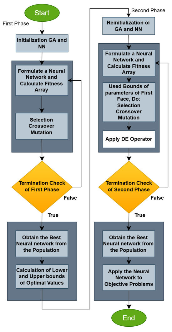
Figure 1. The flowchart of the proposed method.

3. Experiments

To demonstrate the dynamics and reliability of the proposed methodology, a series of experiments were carried out on known datasets from the relevant literature. These datasets were obtained from the following databases:

• The UCI database https://archive.ics.uci.edu/ (accessed on 5 March 2025) [52].
• The Keel website, https://sci2s.ugr.es/keel/datasets.php (accessed on 5 March 2025) [53].
• The Statlib URL https://lib.stat.cmu.edu/datasets/ (accessed on 5 March 2025).

3.1. Experimental Datasets

The following series of classification datasets were used in the conducted experiments:

• The Alcohol dataset, which is related to experiments on alcohol consumption [54].
• The Appendicitis dataset, which is a medical dataset [55].
• The Australian dataset, which is used in bank transactions [56].
• The Balance dataset, which contains measurements from various psychological experiments [57].
• The Circular dataset, which was created artificially.
• The Cleveland dataset, which is a medical dataset [58,59].
• The Dermatology dataset, which is a medical dataset regarding dermatology problems [60].
• The Ecoli dataset, which is used in protein problems [61].
• The Fert dataset, related to the detection of relations between sperm concentration and demographic data.
• The Haberman dataset, which is related to the detection of breast cancer.
• The Hayes roth dataset [62].
• The Heart dataset, which is related to some heart diseases [63].
• The HouseVotes dataset, related to data from congressional voting in USA [64].
• The Ionosphere dataset, that contains measurements from the ionosphere [65,66].
• The Liverdisorder dataset, which is a medical dataset [67,68].
• The Lymography dataset [69].
• The Mammographic dataset, which is a medical dataset [70].
• The Parkinsons dataset, that was used in the detection of Parkinson’s disease [71,72].
• The Pima dataset, a medical dataset related to the detection of diabetes’s disease [73].
• The Popfailures dataset, related to climate model simulations [74].
• The Regions2 dataset, related to some diseases in liver [75].
• The Saheart dataset, related to some heart diseases [76].
• The Segment dataset, related to image processing [77].
• The Sonar dataset, used to discriminate sonar signals [78].
• The Spiral dataset, which was created artificially.
• The StatHeart dataset, a medical dataset regarding heart diseases.
• The Student dataset, which is related to experiments conducted in schools [79].
• The WDBC dataset, which is related to the detection of cancer [80].
• The Wine dataset, used to detection of the quality of wines [81,82].
• The EEG dataset, which contains various EEG measurements [83,84]. From this dataset, the following cases were utilized: Z_F_S, ZO_NF_S and ZONF_S.
• The ZOO dataset, which is used for animal classification [85].

Also, the following regression datasets were incorporated in the conducted experiments:

• The Abalone dataset, that was used to predict the age of abalones [86].
• The Airfoil dataset, derived from NASA [87].
• The Baseball dataset, used to predict the salary of baseball players.
• The BK dataset, related to basketball games [88].
• The BL dataset, related to some electricity experiments.
• The Concrete dataset, which is related to civil engineering [89].
• The Dee dataset, which is related to the price of electricity.
• The Housing dataset, related to the price of houses [90].
• The Friedman dataset, used in various benchmarks [91].
• The FY dataset, related to fruit flies.
• The HO dataset, obtained from the STATLIB repository.
• The Laser dataset, related to laser experiments.
• The LW dataset, related to the prediction of the weight of babes.
• The MB dataset, which was obtained from Smoothing Methods in Statistics.
• The Mortgage dataset, which is an economic dataset.
• The Plastic dataset, related to the pressure in plastics.
• The PY dataset [92].
• The PL dataset, obtained from the STATLIB repository.
• The Quake dataset, used to detect the strength of earthquakes.
• The SN dataset, which is related to trellising and pruning.
• The Stock dataset, used to estimate the price of stocks.
• The Treasury dataset, which is an economic dataset.
• The VE dataset, obtained from the STATLIB repository.

3.2. Experimental Results

The code used in the conducted experiments was written in ANSI C++ and all runs were performed 30 times using a different seed for the random number generator each time. The validation of the experiments was done using the well-known method of 10-fold cross validation. All the experiments were conducted on a Linux machine with 128 GB of ram. In the case of classification datasets, the average classification error is reported in the experimental tables. This error is calculated through the following equation:

$$E_C\left(N(w,x)\right)=100\times {\displaystyle \frac{{\sum }_{i=1}^K\left(\mathrm{class}\left(N\left(w,x_i\right)\right)-y_i\right)}{K}}$$

(4)

where the set $T=\left\{x_i,y_i\right\},i=1,\dots ,K$ denotes the test set of the objective problem. In regression datasets, the average regression error as calculated on the test set is reported and it is denoted as:

$$E_R\left(N(w,x)\right)={\displaystyle \frac{{\sum }_{i=1}^K{\left(N\left(w,x_i\right)-y_i\right)}^2}{K}}$$

(5)

The values for the parameters of the proposed method are shown in Table 1. In the experimental tables, the following notation is used:

Table 1. The values of the experimental parameters.

Parameter	Meaning	Value
$N_g$	Number of generations allowed	200
$N_c$	Number of chromosomes	500
$N_i$	Number of generations before the application of the operator	20
$N_l$	Number of chromosomes where the operator will be applied	20
F	Differential Weight	0.8
CR	Crossover probability	0.9
$p_s$	Selection rate	0.1
$p_m$	Mutation rate	0.05
H	Number of processing nodes	10
a	Margin factor	1.0

• The column DATASET represents the objective problem.
• The column ADAM denotes the incorporation of the ADAM optimizer [93] to train a neural network with $H=10$ processing nodes.
• The column BFGS represents the application of the BFGS optimizer [94] to train a neural network with $H=10$ processing nodes.
• The column GENETIC denotes the usage of a genetic algorithm with the same set of parameters as shown in Table 1 to train an artificial neural network with $H=10$ processing nodes.
• The column NEAT is used for the application of the NEAT method (NeuroEvolution of Augmenting Topologies) [95].
• The row AVERAGE is used for the average classification or regression error for all datasets.

Also, for the comparisons between methods, the Wilcoxon signed-rank test was used, which is a non-parametric test for paired data. Each method (“PROPOSED”, “BFGS”, etc.) was evaluated on the same dataset (dependent measurements), which is why a paired observations test was selected. The Mann–Whitney U test or t-test were not applied, as the former is for independent groups and the latter requires normally distributed data conditions that are not met here due to the use of a non-parametric test.

The experimental results for the classification datasets are shown in Table 2 and the experimental results for the regression datasets are shown in Table 3.

Table 2. Experimental results for the classification datasets mentioned here using a series of machine learning methods. The numbers in the cells represent the average classification error as reported in the corresponding test set.

Dataset	ADAM	BFGS	NEAT	GENETIC	PROPOSED
Alcohol	57.78%	41.50%	66.80%	39.57%	24.79%
Appendicitis	16.50%	18.00%	17.20%	18.10%	15.97%
Australian	35.65%	38.13%	31.98%	32.21%	31.76%
Balance	7.87%	8.64%	23.14%	8.97%	8.39%
Circular	19.95%	6.08%	35.18%	5.99%	3.69%
Cleveland	67.55%	77.55%	53.44%	51.60%	48.10%
Dermatology	26.14%	52.92%	32.43%	30.58%	7.74%
Ecoli	64.43%	69.52%	43.44%	54.67%	47.62%
Fert	23.98%	23.20%	15.37%	28.50%	22.00%
Haberman	29.00%	29.34%	24.04%	28.66%	25.99%
Hayes Roth	59.70%	37.33%	50.15%	56.18%	37.00%
Heart	38.53%	39.44%	39.27%	28.34%	24.79%
HouseVotes	7.48%	7.13%	10.89%	6.62%	5.22%
Ionosphere	16.64%	15.29%	19.67%	15.14%	9.56%
Liverdisorder	41.53%	42.59%	30.67%	31.11%	31.08%
Lymography	29.26%	35.43%	33.70%	23.26%	28.60%
Mammographic	46.25%	17.24%	22.85%	19.88%	16.98%
Parkinsons	24.06%	27.58%	18.56%	18.05%	18.02%
Pima	34.85%	35.59%	34.51%	32.19%	30.44%
Popfailures	5.18%	5.24%	7.05%	5.94%	4.29%
Regions2	29.85%	36.28%	33.23%	29.39%	26.43%
Saheart	34.04%	37.48%	34.51%	34.86%	32.60%
Segment	49.75%	68.97%	66.72%	57.72%	30.00%
Sonar	30.33%	25.85%	34.10%	22.40%	18.78%
Spiral	47.67%	47.99%	48.66%	48.66%	44.20%
Statheart	44.04%	39.65%	44.36%	27.25%	22.72%
Student	5.13%	7.14%	10.20%	5.61%	4.16%
Wdbc	35.35%	29.91%	12.88%	8.56%	7.73%
Wine	29.40%	59.71%	25.43%	19.20%	8.55%
Z_F_S	47.81%	39.37%	38.41%	10.73%	6.46%
ZO_NF_S	47.43%	43.04%	43.75%	21.54%	6.01%
ZONF_S	11.99%	15.62%	5.44%	2.60%	1.79%
ZOO	14.13%	10.70%	20.27%	16.67%	9.07%
AVERAGE	32.70%	33.01%	31.16%	25.48%	20.02%

Table 3. Experimental results for the regression datasets using a series of machine learning methods. The numbers in the cells stand for the average regression error as calculated in the corresponding test set.

Dataset	ADAM	BFGS	GENETIC	NEAT	PROPOSED
Abalone	4.30	5.69	7.17	9.88	4.33
Airfoil	0.005	0.003	0.003	0.067	0.003
Baseball	77.90	119.63	103.60	100.39	67.45
BK	0.03	0.28	0.027	0.15	0.02
BL	0.28	2.55	5.74	0.05	0.002
Concrete	0.078	0.066	0.0099	0.081	0.003
Dee	0.63	2.36	1.013	1.512	0.20
Housing	80.20	97.38	43.26	56.49	26.62
Friedman	22.90	1.263	1.249	19.35	1.33
FY	0.038	0.22	0.65	0.08	0.039
HO	0.035	0.62	2.78	0.169	0.014
Laser	0.03	0.015	0.59	0.084	0.0027
LW	0.028	2.98	1.90	0.17	0.016
MB	0.06	0.129	3.39	0.061	0.048
Mortgage	9.24	8.23	2.41	14.11	0.31
Plastic	11.71	20.32	2.79	20.77	2.20
PL	0.117	0.29	0.28	0.098	0.023
PY	0.09	0.578	105.41	0.075	0.016
Quake	0.06	0.42	0.040	0.298	0.043
SN	0.206	0.40	2.95	0.174	0.024
Stock	180.89	302.43	3.88	215.82	3.47
Treasury	11.16	9.91	2.929	15.52	0.44
VE	0.359	1.92	2.43	0.045	0.023
AVERAGE	17.41	25.12	12.80	19.80	4.64

Also, in Figure 2 and Figure 3, the statistical comparison for the experimental results is outlined graphically.

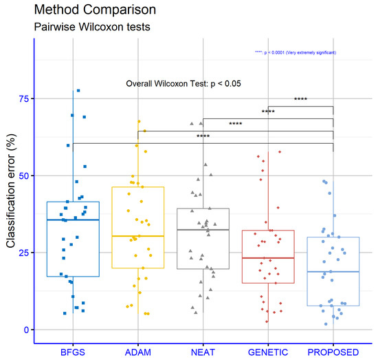
Figure 2. Statistical comparison for the obtained experimental results using a variety of machine learning methods in the classification datasets.

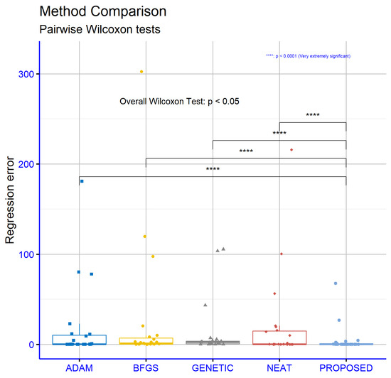
Figure 3. Statistical comparison of the experimental results using a series of machine learning methods on the regression datasets.

In the scientific analysis of the experimental results, the proposed model (PROPOSED) demonstrates statistically significant superiority over other methods (ADAM, BFGS, GENETIC, NEAT, RBF) in both the classification and regression datasets. For classification, the PROPOSED model achieves a mean error rate of 20.02%, compared to 25.48–33.01% for the other methods, with extremely low p-values (e.g., $p=2.3\times {10}^{-10}$ against BFGS). In regression, the model’s mean absolute error (4.64) is significantly lower than that of the comparative methods (12.8–25.12), with strong statistical significance $\left(p<{10}^{-5}\right)$. However, in certain datasets (e.g., CLEVELAND, FRIEDMAN), the model’s performance decreases, indicating dependence on data characteristics.

In the analysis of the experiments (Figure 2) for classification datasets, the proposed model (PROPOSED) demonstrates statistically significant superiority over all comparative methods (BFGS, ADAM, NEAT, GENETIC), with extremely low p-values ($p=2.3\times {10}^{-10}$ to $p=4.4\times {10}^{-6}$). This indicates strong differences at a confidence level >99.9%, particularly against BFGS and ADAM $\left(p<{10}^{-9}\right)$. For regression datasets (Figure 3), PROPOSED maintains significant superiority over all methods, though with slightly higher p-values $\left(p={10}^{-5}\mathrm{t}\mathrm{o}p=2.4\times {10}^{-7}\right)$. The largest difference is observed against NEAT $\left(p=2.4\times {10}^{-7}\right)$, while the smallest is against GENETIC $\left(p=8.6\times {10}^{-5}\right)$.

Moreover, in Figure 4, the a comparison of execution times is graphically outlined between the simple genetic algorithm and the proposed method for various values of the critical parameter $N_I$. The dataset used in this experiment is the WINE classification dataset. As expected, increasing the value of this parameter also leads to a reduction in the required execution time for the proposed method, since the new genetic operator is applied more and more sparsely to the population chromosomes.

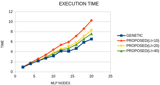
Figure 4. A comparison of execution times for the WINE dataset between the simple genetic algorithm and the proposed method for various values of the parameter $N_I$.

3.3. Experiments with the Differential Weight

An additional experiment was performed to demonstrate the reliability of the proposed methodology. In this experiment, three different differential weight F calculation techniques were used for the proposed operator. The range of this parameter was defined as [0, 2] in the work of Storn and Price [96]. These techniques are the following:

• FIXED, which is the default technique in the proposed method. In this technique, the value $F=0.8$ is used for the differential weight.
• ADAPTIVE, where the adaptive calculation of the parameter F is used as proposed in [97].
• RANDOM, where the stochastic calculation of parameter F as proposed in [98] is used.

In Table 4, the results from the application of the proposed method using the previously mentioned techniques for the differential weight are depicted for the classification datasets. Similarly, the same method is applied to the regression datasets and the results are presented in Table 5.

Table 4. Experiments for classification datasets using a series of differential weight mechanisms.

Dataset	FIXED	ADAPTIVE	RANDOM
Alcohol	24.79%	25.65%	23.02%
Appendicitis	15.97%	15.83%	15.80%
Australian	31.76%	31.61%	31.60%
Balance	8.39%	8.45%	8.65%
Circular	3.69%	3.67%	3.78%
Cleveland	48.10%	48.39%	48.35%
Dermatology	7.74%	7.27%	7.37%
Ecoli	47.62%	48.34%	47.96%
Fert	22.00%	22.17%	22.10%
Haberman	25.99%	26.20%	26.12%
Hayes Roth	37.00%	38.38%	37.65%
Heart	24.79%	24.15%	25.51%
HouseVotes	5.22%	5.21%	4.78%
Ionosphere	9.56%	9.28%	9.30%
Liverdisorder	31.08%	31.46%	31.11%
Lymography	28.60%	28.95%	27.88%
Mammographic	16.98%	17.02%	17.18%
Parkinsons	18.02%	17.86%	17.90%
Pima	30.44%	31.12%	30.48%
Popfailures	4.29%	4.25%	4.28%
Regions2	26.43%	25.94%	26.35%
Saheart	32.60%	33.11%	32.92%
Segment	30.00%	28.83%	30.85%
Sonar	18.78%	18.08%	18.70%
Spiral	44.20%	44.21%	44.12%
Statheart	22.72%	22.72%	23.41%
Student	4.16%	3.95%	4.35%
Wdbc	7.73%	7.48%	7.40%
Wine	8.55%	6.29%	6.74%
Z_F_S	6.46%	6.92%	6.65%
ZO_NF_S	6.01%	6.10%	5.89%
ZONF_S	1.79%	1.71%	1.76%
ZOO	9.07%	6.57%	8.90%
AVERAGE	20.02%	19.91%	19.97%

Table 5. Experiments on regression datasets using a variety of weight mechanism methods.

Dataset	FIXED	ADAPTIVE	RANDOM
ABALONE	4.33	4.24	4.34
AIRFOIL	0.003	0.003	0.003
BASEBALL	67.45	67.23	66.76
BK	0.02	0.02	0.02
BL	0.002	0.002	0.002
CONCRETE	0.003	0.003	0.003
DEE	0.20	0.20	0.20
HOUSING	26.62	26.07	26.11
FRIEDMAN	1.33	1.21	1.34
FY	0.039	0.039	0.039
HO	0.014	0.014	0.014
LASER	0.0027	0.0027	0.0028
LW	0.016	0.011	0.011
MB	0.048	0.048	0.048
MORTGAGE	0.31	0.35	0.34
PLASTIC	2.20	2.13	2.20
PL	0.023	0.022	0.022
PY	0.016	0.017	0.017
QUAKE	0.043	0.082	0.04
SN	0.024	0.024	0.024
STOCK	3.47	3.33	3.45
TREASURY	0.44	0.42	0.45
VE	0.023	0.023	0.023
AVERAGE	4.64	4.59	4.59

Furthermore, the statistical comparison of these experimental tables is outlined in Figure 5 and Figure 6, respectively.

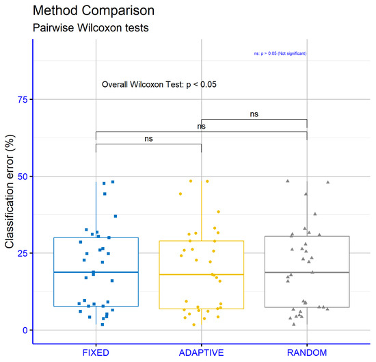
Figure 5. Statistical comparison of the experimental results on the classification datasets, using the proposed method and a series of differential weight techniques.

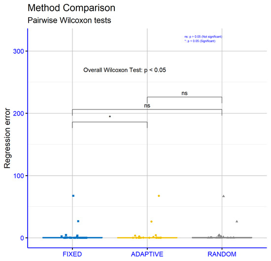
Figure 6. Statistical comparison of the experiments on the regression datasets using the proposed method and a series of differential weight calculation techniques.

When comparing differential weight calculation methods (FIXED, ADAPTIVE, RANDOM), the ADAPTIVE method shows slightly better average performance (19.91% in classification, 4.59 in regression) compared to FIXED (20.02%, 4.64) and RANDOM (19.97%, 4.59). However, the differences are minimal and often statistically insignificant (e.g., $p=0.83$ for FIXED vs. ADAPTIVE in classification). In some datasets, such as Lymography and HouseVotes, the RANDOM method outperforms others, highlighting the need to tailor the method to the specific problem. In regression, the only significant difference occurs between FIXED and ADAPTIVE ($p=0.041$).

For this experiment, as shown in Figure 5, the differences between FIXED and ADAPTIVE ($p=0.83$) and ADAPTIVE vs RANDOM ($p=0.94$) are not statistically significant, suggesting equivalent performance. However, the comparison FIXED vs. RANDOM ($p=2.3\times {10}^{-10}$) reveals a highly significant difference, likely due to the random nature of RANDOM. For regression datasets (Figure 6), the only significant difference occurs between FIXED and ADAPTIVE ($p=0.041$), while the remaining comparisons (FIXED vs. RANDOM: $p=0.75$, ADAPTIVE vs. RANDOM: $p=0.31$) lack statistical significance.

3.4. Experiments with the Margin Factor a

An additional experiment was executed to outline the performance and the stability of the proposed method. In this experiment, the margin factor denoted as a in the proposed method was varied from $a=1.0$ (which is the default value) to $a=4.0$. The experimental results for the classification datasets are shown in Table 6 and regression dataset results are in Table 7.

Table 6. Experiments for classification datasets using a series of values for the margin factor a.

Dataset	$\mathit{a}=1.0$	$\mathit{a}=1.5$	$\mathit{a}=2.0$	$\mathit{a}=2.5$	$\mathit{a}=3.0$	$\mathit{a}=3.5$	$\mathit{a}=4.0$
Alcohol	24.79%	22.88%	25.55%	30.21%	30.77%	32.05%	28.42%
Appendicitis	15.97%	16.33%	18.07%	18.70%	17.30%	18.60%	19.51%
Australian	31.76%	32.79%	33.23%	32.65%	32.87%	32.76%	33.68%
Balance	8.39%	8.50%	8.39%	8.84%	8.85%	8.87%	8.78%
Circular	3.69%	4.19%	4.22%	4.30%	4.33%	4.46%	4.70%
Cleveland	48.10%	47.17%	46.68%	47.58%	50.84%	50.62%	47.74%
Dermatology	7.74%	7.47%	7.60%	7.57%	7.71%	8.86%	7.83%
Ecoli	47.62%	48.69%	48.29%	49.50%	51.39%	51.99%	49.39%
Fert	22.00%	23.47%	23.50%	25.03%	24.80%	24.17%	24.27%
Haberman	25.99%	26.26%	26.74%	27.23%	27.49%	27.67%	27.14%
Hayes Roth	37.00%	39.15%	39.69%	35.49%	38.10%	39.15%	40.05%
Heart	24.79%	24.64%	24.85%	25.50%	26.85%	26.46%	24.89%
HouseVotes	5.22%	4.91%	5.05%	4.90%	4.57%	4.71%	5.02%
Ionosphere	9.56%	9.65%	9.92%	9.72%	9.75%	9.57%	10.23%
Liverdisorder	31.08%	31.94%	31.42%	30.89%	31.54%	30.92%	32.13%
Lymography	28.60%	28.24%	28.79%	30.21%	29.64%	30.71%	26.69%
Mammographic	16.98%	16.34%	16.35%	15.86%	15.88%	16.35%	16.69%
Parkinsons	18.02%	18.88%	18.56%	17.98%	17.74%	17.95%	19.40%
Pima	30.44%	30.89%	31.11%	32.81%	32.88%	32.83%	31.03%
Popfailures	4.29%	5.07%	5.53%	5.51%	5.54%	5.97%	5.97%
Regions2	26.43%	26.53%	26.30%	26.52%	26.28%	26.26%	25.35%
Saheart	32.60%	31.43%	32.98%	33.52%	33.49%	33.46%	32.93%
Segment	30.00%	27.98%	30.86%	31.39%	33.76%	34.51%	35.41%
Sonar	18.78%	21.08%	22.23%	21.47%	21.75%	21.57%	21.68%
Spiral	44.20%	44.65%	44.52%	43.81%	43.58%	43.39%	44.13%
Statheart	22.72%	23.40%	23.85%	24.22%	25.56%	26.10%	24.22%
Student	4.16%	4.75%	5.24%	5.38%	5.43%	5.55%	5.37%
Wdbc	7.73%	6.95%	6.64%	7.14%	7.29%	7.17%	7.31%
Wine	8.55%	6.59%	9.35%	9.47%	8.12%	9.65%	11.02%
Z_F_S	6.46%	6.66%	6.90%	6.92%	6.53%	6.87%	6.61%
ZO_NF_S	6.01%	6.03%	6.08%	6.95%	7.17%	7.28%	6.25%
ZONF_S	1.79%	1.75%	1.80%	2.15%	2.14%	2.13%	1.79%
ZOO	9.07%	8.63%	7.00%	7.87%	6.77%	6.97%	7.53%
AVERAGE	20.02%	20.12%	20.52%	20.83%	21.11%	21.38%	21.00%

Table 7. Experiments for regression datasets using a variety of values for the margin factor a.

Dataset	$\mathit{a}=1.0$	$\mathit{a}=1.5$	$\mathit{a}=2.0$	$\mathit{a}=2.5$	$\mathit{a}=3.0$	$\mathit{a}=3.5$	$\mathit{a}=4.0$
ABALONE	4.33	4.39	4.46	4.64	4.84	4.93	5.06
AIRFOIL	0.003	0.003	0.002	0.002	0.003	0.003	0.002
BASEBALL	67.45	74.66	79.78	79.39	81.55	84.65	86.54
BK	0.02	0.019	0.019	0.018	0.017	0.018	0.02
BL	0.002	0.001	0.001	0.0007	0.0009	0.0008	0.003
CONCRETE	0.003	0.003	0.003	0.004	0.003	0.004	0.003
DEE	0.20	0.20	0.20	0.21	0.20	0.21	0.20
HOUSING	26.62	26.24	28.13	27.91	27.36	29.53	29.25
FRIEDMAN	1.33	1.19	1.20	1.21	1.22	1.21	1.20
FY	0.039	0.04	0.042	0.041	0.042	0.042	0.045
HO	0.014	0.014	0.013	0.013	0.013	0.014	0.014
LASER	0.0027	0.0025	0.0025	0.0028	0.0026	0.0025	0.0024
LW	0.016	0.011	0.011	0.013	0.013	0.014	0.013
MB	0.048	0.049	0.051	0.051	0.052	0.054	0.09
MORTGAGE	0.31	0.21	0.37	0.48	0.63	0.68	0.62
PLASTIC	2.20	2.05	2.18	2.23	2.25	2.23	2.21
PL	0.023	0.023	0.021	0.022	0.022	0.022	0.022
PY	0.016	0.022	0.023	0.026	0.028	0.027	0.028
QUAKE	0.043	0.038	0.04	0.039	0.037	0.037	0.039
SN	0.024	0.024	0.025	0.024	0.026	0.024	0.026
STOCK	3.47	3.59	3.68	3.70	3.37	3.24	3.35
TREASURY	0.44	0.42	0.40	0.65	0.82	0.95	1.01
VE	0.023	0.024	0.024	0.025	0.026	0.027	0.029
AVERAGE	4.64	4.92	5.25	5.25	5.33	5.56	5.64

Also, the statistical comparisons for these experiments are shown graphically in Figure 7 and Figure 8, respectively.

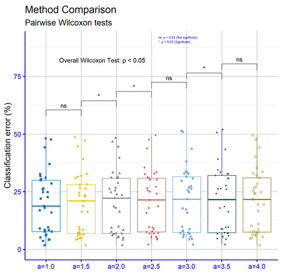
Figure 7. Statistical comparison of the experimental results on the classification datasets using the proposed method and different values for the margin factor a.

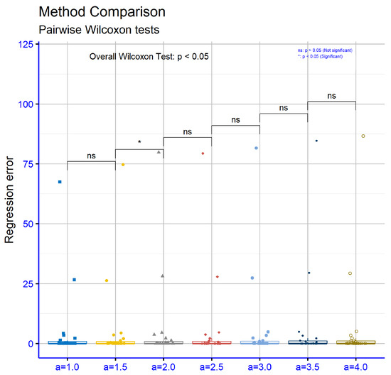
Figure 8. Statistical comparison of the experiments on the regression datasets using the proposed method and different values for the margin factor a.

Table 6 presents the percentage error values corresponding to various classification datasets for different values of the parameter a, which determines the optimal value boundaries in the proposed machine learning model. The last row of the table includes the average error for each value of the parameter a. The data analysis reveals that an increase in the parameter a generally leads to a rise in the average error rate. Specifically, the average increases from 20.02% for $\alpha =1.0$ to 21.38% for $\alpha =3.5$, while for $\alpha =4.0$, it slightly decreases to 21.00%. This indicates that, despite the general upward trend, there are cases where further increasing the parameter can reduce the error. A detailed examination of the data by dataset shows significant variations among different values of the parameter a. For example, in the Circular dataset, the error gradually increases from 3.69% for $\alpha =1.0$ to 4.70% for $\alpha =4.0$. Similarly, in the Wine dataset, the error value increases from 8.55% for $\alpha =1.0$ to 11.02% for $\alpha =4.0$, indicating a clear negative impact of increasing the parameter. However, in other datasets, the effect of the parameter is neither as linear nor as pronounced. For instance, in the Hayes Roth dataset, the error decreases from 39.69% for $\alpha =2.0$ to 35.49% for $\alpha =2.5$, before increasing again. Similarly, in the Lymography dataset, the error significantly decreases for $\alpha =4.0$ (26.69%) compared to the other parameter values. These data demonstrate that the relationship between the parameter a and the error is not linear across all datasets and depends on the specific characteristics of each dataset. Overall, the statistical analysis indicates that while increasing the parameter a is often associated with higher errors, there are exceptions that may be linked to specific properties of the data or the model.

Table 7 presents the absolute error values for various regression datasets in relation to different values of the parameter a, which determines the optimal value boundaries in the proposed machine learning model. The last row lists the average errors for each value of the parameter a. The table analysis shows that an increase in the parameter a is accompanied by a general increase in the average error. Specifically, the average error increases from 4.64 for $\alpha =1.0$ to 5.64 for $\alpha =4.0$, suggesting that higher parameter values may lead to worse model performance. Examining the individual datasets reveals variability in the effect of the parameter a. For example, in the BASEBALL dataset, the error continuously increases from 67.45 for $\alpha =1.0$ to 86.54 for $\alpha =4.0$, indicating a clear negative effect of increasing the parameter. Conversely, in the STOCK dataset, an increase in the parameter is accompanied by a decrease in error, from 3.47 for $\alpha =1.0$ to 3.35 for $\alpha =4.0$. In other datasets, the effect is less straightforward. For example, in the MORTGAGE dataset, the error increases from 0.31 for $\alpha =1.0$ to 0.68 for $\alpha =3.5$ but slightly decreases to 0.62 for $\alpha =4.0$. Overall, the statistical analysis suggests that the effect of the parameter a depends on the characteristics of each dataset and that, although increasing the parameter is often associated with higher errors, there are cases where performance remains stable or improves slightly.

In Figure 7, the results pertain to classification datasets and various models. From the comparisons between different values of the parameter a, it is observed that the comparison between $a=1.0$ and $a=1.5$ does not exhibit a statistically significant difference ($p=0.38$). In contrast, the comparison between $a=1.5$ and $a=2.0$ shows a significant difference ($p=0.018$), as does the comparison between $a=2.0$ and $a=2.5$ ($p=0.045$). The remaining comparisons, specifically between $a=2.5$ and $a=3.0$ ($p=0.25$), $a=3.0$ and $a=3.5$ ($p=0.27$), and $a=3.5$ and $a=4.0$ ($p=0.39$), do not demonstrate statistically significant differences.

In Figure 8, the data refer to regression datasets and comparisons for various models. The results indicate that the comparison between $a=1.0$ and $a=1.5$ is not statistically significant ($p=0.55$), whereas the difference between $a=1.5$ and $a=2.0$ is statistically significant ($p=0.014$). The comparison between $a=2.0$ and $a=2.5$ does not show statistical significance ($p=0.17$), nor do the comparisons between $a=2.5$ and $a=3.0$ ($p=0.2$), $a=3.0$ and $a=3.5$ ($p=0.16$), and $a=3.5$ and $a=4.0$ ($p=0.31$). Overall, the p values highlight significant differences in specific cases, while in others, the differences remain statistically insignificant.

4. Conclusions

The study confirms the superiority of the proposed model compared to existing methods in both classification and regression tasks. This superiority is demonstrated by a statistically significant reduction in error, although the model’s performance heavily depends on data characteristics such as complexity, stratification, or the presence of noise. This highlights the importance of adapting the model to the specificities of each problem, as overly generalized approaches may lead to suboptimal results. Additionally, the choice of methods for calculating critical parameters, such as differential weights, appears to have a relatively limited impact on overall performance. Differences between approaches (e.g., FIXED, ADAPTIVE, RANDOM) are minimal and often statistically insignificant, suggesting that optimization efforts could focus on other factors. Tuning the parameter “a”, however, emerges as a critical factor. Higher values of this parameter often improve accuracy, particularly for large or complex datasets, but they may also introduce instability in applications where data sensitivity is high (e.g., financial forecasting). This dual behavior underscores the need to balance flexibility and robustness during the tuning process. Despite its analytical approach, the study does not sufficiently explore the potential real-world applications of the proposed model beyond benchmark datasets. Addressing this gap, future research could expand the methodology to practical domains such as biomedical data analysis, social networks, or dynamic systems, including real-time monitoring and financial forecasting. Investigating the model’s adaptability and scalability in these fields could enhance its utility in real-world scenarios.

For future research, it would be beneficial to develop dynamic algorithms that automatically adjust the parameter a based on data dynamics. For example, machine learning mechanisms that analyze data variability or heterogeneity in real-time could optimize the value of a without human intervention, ensuring both stability and high performance. Additionally, the development of hybrid methods that combine the adaptability of ADAPTIVE approaches with the simplicity of FIXED approaches could result in more resilient solutions capable of addressing a broader range of problems. It is also important to investigate how specific data characteristics—such as noisy measurements, class imbalances, or lack of labeling—affect the model’s effectiveness. Such an analysis would support the development of adaptive strategies for data preprocessing or augmentation. Furthermore, exploring the generalizability of results to more complex environments, such as time-series data or dynamic systems, remains an open research avenue. Finally, integrating explainable artificial intelligence (XAI) techniques, such as feature contribution analysis or visualization tools, could enhance the model’s transparency. This would not only facilitate the interpretation of results by experts but also aid in identifying optimal parameter-tuning practices, making the model a more predictable and reliable tool for real-world applications.

References

- Abiodun, O.I.; Jantan, A.; Omolara, A.E.; Dada, K.V.; Mohamed, N.A.; Arshad, H. State-of-the-art in artificial neural network applications: A survey. Heliyon 2018, 4, e00938. [Google Scholar]
- Suryadevara, S.; Yanamala, A.K.Y. A Comprehensive Overview of Artificial Neural Networks: Evolution, Architectures, and Applications. Rev. Intel. Artif. Med. 2021, 12, 51–76. [Google Scholar]
- Baldi, P.; Cranmer, K.; Faucett, T.; Sadowski, P.; Whiteson, D. Parameterized neural networks for high-energy physics. Eur. Phys. J. C 2016, 76, 235. [Google Scholar]
- Firth, A.E.; Lahav, O.; Somerville, R.S. Estimating photometric redshifts with artificial neural networks. Mon. Not. R. Astron. Soc. 2003, 339, 1195–1202. [Google Scholar] [CrossRef]
- Shen, Y.; Bax, A. Protein backbone and sidechain torsion angles predicted from NMR chemical shifts using artificial neural networks. J. Biomol. NMR 2013, 56, 227–241. [Google Scholar]
- Huang, Z.; Chen, H.; Hsu, C.-J.; Chen, W.-H.; Wu, S. Credit rating analysis with support vector machines and neural networks: A market comparative study. Decis. Support Syst. 2004, 37, 543–558. [Google Scholar]
- Baskin, I.I.; Winkler, D.; Tetko, I.V. A renaissance of neural networks in drug discovery. Expert Opin. Drug Discov. 2016, 11, 785–795. [Google Scholar]
- Bartzatt, R. Prediction of Novel Anti-Ebola Virus Compounds Utilizing Artificial Neural Network (ANN). Chem. Fac. Publ. 2018, 49, 16–34. [Google Scholar]
- Rumelhart, D.E.; Hinton, G.E.; Williams, R.J. Learning representations by back-propagating errors. Nature 1986, 323, 533–536. [Google Scholar]
- Chen, T.; Zhong, S. Privacy-Preserving Backpropagation Neural Network Learning. IEEE Trans. Neural Netw. 2009, 20, 1554–1564. [Google Scholar]
- Riedmiller, M.; Braun, H. A Direct Adaptive Method for Faster Backpropagation Learning: The RPROP algorithm. In Proceedings of the IEEE International Conference on Neural Networks, San Francisco, CA, USA, 28 March–1 April 1993; pp. 586–591. [Google Scholar]
- Pajchrowski, T.; Zawirski, K.; Nowopolski, K. Neural Speed Controller Trained Online by Means of Modified RPROP Algorithm. IEEE Trans. Ind. Inform. 2015, 11, 560–568. [Google Scholar]
- Hermanto, R.P.S.; Suharjito; Diana; Nugroho, A. Waiting-Time Estimation in Bank Customer Queues using RPROP Neural Networks. Procedia Comput. Sci. 2018, 135, 35–42. [Google Scholar]
- Robitaille, B.; Marcos, B.; Veillette, M.; Payre, G. Modified quasi-Newton methods for training neural networks. Comput. Chem. Eng. 1996, 20, 1133–1140. [Google Scholar]
- Liu, Q.; Liu, J.; Sang, R.; Li, J.; Zhang, T.; Zhang, Q. Fast Neural Network Training on FPGA Using Quasi-Newton Optimization Method. IEEE Trans. Very Large Scale Integr. (Vlsi) Syst. 2018, 26, 1575–1579. [Google Scholar]
- Kuo, C.L.; Kuruoglu, E.E.; Chan, W.K.V. Neural Network Structure Optimization by Simulated Annealing. Entropy 2022, 24, 348. [Google Scholar] [CrossRef]
- Zhang, C.; Shao, H.; Li, Y. Particle swarm optimization for evolving artificial neural network. In Proceedings of the IEEE International Conference on Systems, Man, and Cybernetics, Nashville, TN, USA, 8–11 October 2000; pp. 2487–2490. [Google Scholar]
- Yu, J.; Wang, S.; Xi, L. Evolving artificial neural networks using an improved PSO and DPSO. Neurocomputing 2008, 71, 1054–1060. [Google Scholar]
- Leung, F.H.F.; Lam, H.K.; Ling, S.H.; Tam, P.K.S. Tuning of the structure and parameters of a neural network using an improved genetic algorithm. IEEE Trans. Neural Netw. 2003, 14, 79–88. [Google Scholar] [PubMed]
- Yao, X. Evolving artificial neural networks. Proc. IEEE 1999, 87, 1423–1447. [Google Scholar]
- Wang, L.; Zeng, Y.; Chen, T. Back propagation neural network with adaptive differential evolution algorithm for time series forecasting. Expert Syst. Appl. 2015, 42, 855–863. [Google Scholar]
- Salama, K.M.; Abdelbar, A.M. Learning neural network structures with ant colony algorithms. Swarm Intell. 2015, 9, 229–265. [Google Scholar]
- Mirjalili, S. How effective is the Grey Wolf optimizer in training multi-layer perceptrons. Appl. Intell. 2015, 43, 150–161. [Google Scholar] [CrossRef]
- Aljarah, I.; Faris, H.; Mirjalili, S. Optimizing connection weights in neural networks using the whale optimization Algorithm. Soft Comput. 2018, 22, 1–15. [Google Scholar] [CrossRef]
- Zhang, J.-R.; Zhang, J.; Lok, T.-M.; Lyu, M.R. A hybrid particle swarm optimization–back-propagation algorithm for feedforward neural network training. Appl. Math. Comput. 2007, 185, 1026–1037. [Google Scholar] [CrossRef]
- Oh, K.S.; Jung, K. GPU implementation of neural networks. Pattern Recognit. 2004, 37, 1311–1314. [Google Scholar] [CrossRef]
- Zhang, M.; Hibi, K.; Inoue, J. GPU-accelerated artificial neural network potential for molecular dynamics simulation. Comput. Phys. Commun. 2023, 285, 108655. [Google Scholar]
- Krüger, T.; Kusumaatmaja, H.; Kuzmin, A.; Shardt, O.; Silva, G.; Viggen, E.M. The Lattice Boltzmann Method; Springer International Publishing: Berlin/Heidelberg, Germany, 2017; Volume 10, pp. 4–15. [Google Scholar]
- Kang, Q.; Li, K.Q.; Fu, J.L.; Liu, Y. Hybrid LBM and machine learning algorithms for permeability prediction of porous media: A comparative study. Comput. Geotech. 2024, 168, 106163. [Google Scholar] [CrossRef]
- Ivanova, I.; Kubat, M. Initialization of neural networks by means of decision trees. Knowl.-Based Syst. 1995, 8, 333–344. [Google Scholar]
- Yam, J.Y.F.; Chow, T.W.S. A weight initialization method for improving training speed in feedforward neural network. Neurocomputing 2000, 30, 219–232. [Google Scholar] [CrossRef]
- Chumachenko, K.; Iosifidis, A.; Gabbouj, M. Feedforward neural networks initialization based on discriminant learning. Neural Netw. 2022, 146, 220–229. [Google Scholar]
- Varnava, T.M.; Meade, A.J. An initialization method for feedforward artificial neural networks using polynomial bases. Adv. Adapt. Data Anal. 2011, 3, 385–400. [Google Scholar]
- Sodhi, S.S.; Chandra, P. Interval based Weight Initialization Method for Sigmoidal Feedforward Artificial Neural Networks. AASRI Procedia 2014, 6, 19–25. [Google Scholar]
- Narkhede, M.V.; Bartakke, P.P.; Sutaone, M.S. A review on weight initialization strategies for neural networks. Artif. Intell. Rev. 2022, 55, 291–322. [Google Scholar]
- Arifovic, J.; Gençay, R. Using genetic algorithms to select architecture of a feedforward artificial neural network. Phys. A Stat. Mech. Its Appl. 2001, 289, 574–594. [Google Scholar] [CrossRef]
- Benardos, P.G.; Vosniakos, G.C. Optimizing feedforward artificial neural network architecture. Eng. Appl. Artif. Intell. 2007, 20, 365–382. [Google Scholar]
- Garro, B.A.; Vázquez, R.A. Designing Artificial Neural Networks Using Particle Swarm Optimization Algorithms. Comput. Neurosci. 2015, 2015, 369298. [Google Scholar] [CrossRef]
- Baker, B.; Gupta, O.; Naik, N.; Raskar, R. Designing neural network architectures using reinforcement learning. arXiv 2016, arXiv:1611.02167. [Google Scholar]
- O’Neill, M.; Ryan, C. Grammatical evolution. IEEE Trans. Evol. Comput. 2001, 5, 349–358. [Google Scholar]
- Tsoulos, I.G.; Gavrilis, D.; Glavas, E. Neural network construction and training using grammatical evolution. Neurocomputing 2008, 72, 269–277. [Google Scholar]
- Pant, M.; Zaheer, H.; Garcia-Hernandez, L.; Abraham, A. Differential Evolution: A review of more than two decades of research. Eng. Appl. Artif. Intell. 2020, 90, 103479. [Google Scholar]
- Li, Y.H.; Wang, J.Q.; Wang, X.J.; Zhao, Y.L.; Lu, X.H.; Liu, D.L. Community detection based on differential evolution using social spider optimization. Symmetry 2017, 9, 183. [Google Scholar] [CrossRef]
- Yang, W.; Siriwardane EM, D.; Dong, R.; Li, Y.; Hu, J. Crystal structure prediction of materials with high symmetry using differential evolution. J. Phys. Condens. Matter 2021, 33, 455902. [Google Scholar]
- Lee, C.Y.; Hung, C.H. Feature ranking and differential evolution for feature selection in brushless DC motor fault diagnosis. Symmetry 2021, 13, 1291. [Google Scholar] [CrossRef]
- Saha, S.; Das, R. Exploring differential evolution and particle swarm optimization to develop some symmetry-based automatic clustering techniques: Application to gene clustering. Neural Comput. Appl. 2018, 30, 735–757. [Google Scholar] [CrossRef]
- Grady, S.A.; Hussaini, M.Y.; Abdullah, M.M. Placement of wind turbines using genetic algorithms. Renew. Energy 2005, 30, 259–270. [Google Scholar] [CrossRef]
- Prasad, T.; Park, N. Multiobjective Genetic Algorithms for Design of Water Distribution Networks. J. Water Resour. Plann. Manag. 2004, 130, 73–82. [Google Scholar] [CrossRef]
- Min, S.-H.; Lee, J.; Han, I. Hybrid genetic algorithms and support vector machines for bankruptcy prediction. Expert Syst. Appl. 2006, 31, 652–660. [Google Scholar] [CrossRef]
- Whitley, D.; Starkweather, T.; Bogart, C. Genetic algorithms and neural networks: Optimizing connections and connectivity. Parallel Comput. 1990, 14, 347–361. [Google Scholar] [CrossRef]
- Kaelo, P.; Ali, M.M. Integrated crossover rules in real coded genetic algorithms. Eur. J. Oper. Res. 2007, 176, 60–76. [Google Scholar] [CrossRef]
- Kelly, M.; Longjohn, R.; Nottingham, K. The UCI Machine Learning Repository. 2023. Available online: https://archive.ics.uci.edu (accessed on 20 September 2023).
- Alcalá-Fdez, J.; Fernandez, A.; Luengo, J.; Derrac, J. García, S.; Sánchez, L.; Herrera, F. KEEL Data-Mining Software Tool: Data Set Repository, Integration of Algorithms and Experimental Analysis Framework. J.-Mult.-Valued Log. Soft Comput. 2011, 17, 255–287. [Google Scholar]
- Tzimourta, K.D.; Tsoulos, I.; Bilero, I.T.; Tzallas, A.T.; Tsipouras, M.G.; Giannakeas, N. Direct Assessment of Alcohol Consumption in Mental State Using Brain Computer Interfaces and Grammatical Evolution. Inventions 2018, 3, 51. [Google Scholar] [CrossRef]
- Weiss, S.M.; Kulikowski, C.A. Computer Systems That Learn: Classification and Prediction Methods from Statistics, Neural Nets, Machine Learning, and Expert Systems; Morgan Kaufmann Publishers Inc.: Burlington, MA, USA, 1991. [Google Scholar]
- Quinlan, J.R. Simplifying Decision Trees. Int. J.-Man-Mach. Stud. 1987, 27, 221–234. [Google Scholar]
- Shultz, T.; Mareschal, D.; Schmidt, W. Modeling Cognitive Development on Balance Scale Phenomena. Mach. Learn. 1994, 16, 59–88. [Google Scholar]
- Zhou, Z.H.; Jiang, Y. NeC4.5: Neural ensemble based C4.5. IEEE Trans. Knowl. Data Eng. 2004, 16, 770–773. [Google Scholar]
- Setiono, R.; Leow, W.K. FERNN: An Algorithm for Fast Extraction of Rules from Neural Networks. Appl. Intell. 2000, 12, 15–25. [Google Scholar]
- Demiroz, G.; Govenir, H.A.; Ilter, N. Learning Differential Diagnosis of Eryhemato-Squamous Diseases using Voting Feature Intervals. Artif. Intell. Med. 1998, 13, 147–165. [Google Scholar]
- Horton, P.; Nakai, K. A Probabilistic Classification System for Predicting the Cellular Localization Sites of Proteins. Proc. Int. Conf. Intell. Syst. Mol. Biol. 1996, 4, 109–115. [Google Scholar]
- Hayes-Roth, B.; Hayes-Roth, F. Concept learning and the recognition and classification of exemplars. J. Verbal Learn. Verbal Behav. 1977, 16, 321–338. [Google Scholar]
- Kononenko, I.; Šimec, E.; Robnik-Šikonja, M. Overcoming the Myopia of Inductive Learning Algorithms with RELIEFF. Appl. Intell. 1997, 7, 39–55. [Google Scholar]
- French, R.M.; Chater, N. Using noise to compute error surfaces in connectionist networks: A novel means of reducing catastrophic forgetting. Neural Comput. 2002, 14, 1755–1769. [Google Scholar] [PubMed]
- Dy, J.G.; Brodley, C.E. Feature Selection for Unsupervised Learning. J. Mach. Learn. Res. 2004, 5, 845–889. [Google Scholar]
- Perantonis, S.J.; Virvilis, V. Input Feature Extraction for Multilayered Perceptrons Using Supervised Principal Component Analysis. Neural Process. Lett. 1999, 10, 243–252. [Google Scholar]
- Garcke, J.; Griebel, M. Classification with sparse grids using simplicial basis functions. Intell. Data Anal. 2002, 6, 483–502. [Google Scholar]
- Mcdermott, J.; Forsyth, R.S. Diagnosing a disorder in a classification benchmark. Pattern Recognit. Lett. 2016, 73, 41–43. [Google Scholar]
- Cestnik, G.; Konenenko, I.; Bratko, I. Assistant-86: A Knowledge-Elicitation Tool for Sophisticated Users. In Progress in Machine Learning; Bratko, I., Lavrac, N., Eds.; Sigma Press: Wilmslow, UK, 1987; pp. 31–45. [Google Scholar]
- Elter, M.; Schulz-Wendtland, R.; Wittenberg, T. The prediction of breast cancer biopsy outcomes using two CAD approaches that both emphasize an intelligible decision process. Med. Phys. 2007, 34, 4164–4172. [Google Scholar] [PubMed]
- Little, M.; Mcsharry, P.; Roberts, S.; Costello, D.; Moroz, I. et al, Exploiting Nonlinear Recurrence and Fractal Scaling Properties for Voice Disorder Detection. BioMed Eng. OnLine 2007, 6, 23. [Google Scholar]
- Little, M.A.; McSharry, P.E.; Hunter, E.J.; Spielman, J.; Ramig, L.O. Suitability of dysphonia measurements for telemonitoring of Parkinson’s disease. IEEE Trans. Biomed. Eng. 2009, 56, 1015–1022. [Google Scholar]
- Smith, J.W.; Everhart, J.E.; Dickson, W.C.; Knowler, W.C.; Johannes, R.S. Using the ADAP learning algorithm to forecast the onset of diabetes mellitus. In Proceedings of the Symposium on Computer Applications and Medical Care IEEE Computer Society Press, Minneapolis, MN, USA, 8–10 June 1988; pp. 261–265. [Google Scholar]
- Lucas, D.D.; Klein, R.; Tannahill, J.; Ivanova, D.; Brandon, S.; Domyancic, D.; Zhang, Y. Failure analysis of parameter-induced simulation crashes in climate models. Geosci. Dev. 2013, 6, 1157–1171. [Google Scholar]
- Giannakeas, N.; Tsipouras, M.G.; Tzallas, A.T.; Kyriakidi, K.; Tsianou, Z.E.; Manousou, P.; Hall, A.; Karvounis, E.C.; Tsianos, V.; Tsianos, E. A clustering based method for collagen proportional area extraction in liver biopsy images. Annu. Int. Conf. IEEE Eng. Med. Biol. Soc. 2015, 2015, 3097–3100. [Google Scholar]
- Hastie, T.; Tibshirani, R. Non-parametric logistic and proportional odds regression. JRSS-C (Appl. Stat.) 1987, 36, 260–276. [Google Scholar]
- Dash, M.; Liu, H.; Scheuermann, P.; Tan, K.L. Fast hierarchical clustering and its validation. Data Knowl. Eng. 2003, 44, 109–138. [Google Scholar]
- Gorman, R.P.; Sejnowski, T.J. Analysis of Hidden Units in a Layered Network Trained to Classify Sonar Targets. Neural Netw. 1988, 1, 75–89. [Google Scholar]
- Cortez, P.; Silva, A.M.G. Using data mining to predict secondary school student performance. In Proceedings of the 5th FUture BUsiness TEChnology Conference (FUBUTEC 2008), EUROSIS-ETI, Porto, Portugal, 9–11 April 2008; pp. 5–12. [Google Scholar]
- Wolberg, W.H.; Mangasarian, O.L. Multisurface method of pattern separation for medical diagnosis applied to breast cytology. Proc. Natl. Acad. Sci. USA 1990, 87, 9193–9196. [Google Scholar] [PubMed]
- Raymer, M.; Doom, T.E.; Kuhn, L.A.; Punch, W.F. Knowledge discovery in medical and biological datasets using a hybrid Bayes classifier/evolutionary algorithm. IEEE Trans. Syst. Man Cybern. Part B Cybern. 2003, 33, 802–813. [Google Scholar]
- Zhong, P.; Fukushima, M. Regularized nonsmooth Newton method for multi-class support vector machines. Optim. Methods And Softw. 2007, 22, 225–236. [Google Scholar]
- Andrzejak, R.G.; Lehnertz, K.; Mormann, F.; Rieke, C.; David, P.; Elger, C.E. Indications of nonlinear deterministic and finite-dimensional structures in time series of brain electrical activity: Dependence on recording region and brain state. Phys. Rev. E 2001, 64, 061907. [Google Scholar]
- Tzallas, A.T.; Tsipouras, M.G.; Fotiadis, D.I. Automatic Seizure Detection Based on Time-Frequency Analysis and Artificial Neural Networks. Comput. Intell. Neurosci. 2007, 2007, 80510. [Google Scholar] [CrossRef]
- Koivisto, M.; Sood, K. Exact Bayesian Structure Discovery in Bayesian Networks. J. Mach. Learn. Res. 2004, 5, 549–573. [Google Scholar]
- Nash, W.J.; Sellers, T.L.; Talbot, S.R.; Cawthor, A.J.; Ford, W.B. The Population Biology of Abalone (_Haliotis_ Species) in Tasmania. I. Blacklip Abalone (_H. rubra_) from the North Coast and Islands of Bass Strait; Sea Fisheries Division; Technical Report No. 48; Department of Primary Industry and Fisheries, Tasmania: Hobart, Australia, 1994; ISSN 1034-3288. [Google Scholar]
- Brooks, T.F.; Pope, D.S.; Marcolini, A.M. Airfoil Self-Noise and Prediction. Technical Report, NASA RP-1218. July 1989. Available online: https://ntrs.nasa.gov/citations/19890016302 (accessed on 5 March 2025).
- Simonoff, J.S. Smooting Methods in Statistics; Springer: Berlin/Heidelberg, Germany, 1996. [Google Scholar]
- Yeh, I.C. Modeling of strength of high performance concrete using artificial neural networks. Cem. Concr. Res. 1998, 28, 1797–1808. [Google Scholar]
- Harrison, D.; Rubinfeld, D.L. Hedonic prices and the demand for clean ai. J. Environ. Econ. Manag. 1978, 5, 81–102. [Google Scholar]
- Friedman, J. Multivariate Adaptative Regression Splines. Ann. Stat. 1991, 19, 1–141. [Google Scholar]
- King, R.D.; Muggleton, S.; Lewis, R.; Sternberg, M.J.E. Drug design by machine learning: The use of inductive logic programming to model the structure-activity relationships of trimethoprim analogues binding to dihydrofolate reductase. Proc. Nat. Acad. Sci. USA 1992, 89, 11322–11326. [Google Scholar] [PubMed]
- Kingma, D.P.; Ba, J.L. ADAM: A method for stochastic optimization. In Proceedings of the 3rd International Conference on Learning Representations (ICLR 2015), San Diego, CA, USA, 7–9 May 2015; pp. 1–15. [Google Scholar]
- Powell, M.J.D. A Tolerant Algorithm for Linearly Constrained Optimization Calculations. Math. Program. 1989, 45, 547–566. [Google Scholar]
- Stanley, K.O.; Miikkulainen, R. Evolving Neural Networks through Augmenting Topologies. Evol. Comput. 2002, 10, 99–127. [Google Scholar] [PubMed]
- Storn, R.; Price, K. Differential evolution–a simple and efficient heuristic for global optimization over continuous spaces. J. Glob. Optim. 1997, 11, 341–359. [Google Scholar]
- Wu, K.; Liu, Z.; Ma, N.; Wang, D. A Dynamic Adaptive Weighted Differential Evolutionary Algorithm. Comput. Neurosci. 2022, 2022, 1318044. [Google Scholar]
- Charilogis, V.; Tsoulos, I.G.; Tzallas, A.; Karvounis, E. Modifications for the Differential Evolution Algorithm. Symmetry 2022, 14, 447. [Google Scholar] [CrossRef]
Disclaimer/Publisher’s Note: The statements, opinions and data contained in all publications are solely those of the individual author(s) and contributor(s) and not of MDPI and/or the editor(s). MDPI and/or the editor(s) disclaim responsibility for any injury to people or property resulting from any ideas, methods, instructions or products referred to in the content. |
© 2025 by the authors. Licensee MDPI, Basel, Switzerland. This article is an open access article distributed under the terms and conditions of the Creative Commons Attribution (CC BY) license (https://creativecommons.org/licenses/by/4.0/).