Software Reliability Prediction Based on Recurrent Neural Network and Ensemble Method

Abstract

Software reliability is a crucial factor in determining software quality quantitatively. It is also used to estimate the software testing duration. In software reliability testing, traditional parametric software reliability growth models (SRGMs) are effectively used. Nevertheless, a single parametric model cannot provide accurate predictions in all cases. Moreover, non-parametric models have proven to be efficient for predicting software reliability as alternatives to parametric models. In this paper, we adopted a deep learning method for software reliability testing in computer vision systems. Also, we focused on critical computer vision applications that need high reliability. We propose a new deep learning-based model that is combined and based on the ensemble method to improve the performance of software reliability testing. The experimental results of the new model architecture present fairly accurate predictive capability compared to other existing single Neural Network (NN) based models.

1. Introduction

Computer vision is an area of the artificial intelligence field used to train computers to recognize the visual world. The enormous amount of data that is generated today leads to the evolution of computer vision. Computer vision is being used in many areas from early cancer detection to automatic checkouts in retail places. There are various computer vision applications such as face recognition which is used in Facebook, Instagram, Snapchat, and different social media applications. These applications recognize the face in the pictures using face detection algorithms. In the security arena, surveillance cameras detect doubtful behavior in public and private places with the help of computer vision tools. There are different applications in the security area such as facial authentication, fire detection, weapon or dangerous object detection, traffic incident detection, vehicle identification, anomaly detection and credit card fraud detection. Fingerprint and iris recognition are popular applications that use computer vision in biometric identification areas. Most computer vision applications are critical and there is a need to reduce the time required to develop these applications. The computer has a significant role in our current civilization. Software manages critical computer vision systems; so, the software must be reliable and fault free.

Software reliability refers to the probability that software will execute without failure for a given duration within a particular environment [1]. It is significant in the software development process. As the size and complexity of software products have grown quickly, software reliability prediction has become essential for ensuring the development of high-quality software systems. It is particularly valuable for managing software quality and ensuring reliable performance in real-world applications. In the literature, various SRGMs are proposed to estimate the number of future failures and improve the testing efficiency during the software development process [2]. There are two types of SRGMs: parametric models and non-parametric models. In parametric models such as the Nonhomogeneous Poisson Process (NHPP) model, the reliability parameters are estimated based on specific presumptions about the development environments. Nevertheless, it has been proven that a single model cannot obtain accurate predictions for all cases [3,4]. In contrast, non-parametric models such as Neural networks predict the reliability parameters only using fault history, without depending on parametric model presumptions. Neural networks have more flexibility and can provide more accurate predictions for software reliability than parametric models.

The software can encounter failures during its execution [2]. The software failure process is depicted in Figure 1, where t_i represents the execution time for ith software failure and ∆ t_i = t_i − t_i-1 denotes the period between the (i − 1)th and ith software failures. The software reliability data is typically organized in pairs as {ti,Ni}, where Ni represents the cumulative number of failures in the software execution time ti. An example of this software reliability data is illustrated in Figure 2. Using the software’s fault history, software reliability prediction aims to precisely predict the number of failures that may occur during future execution times.

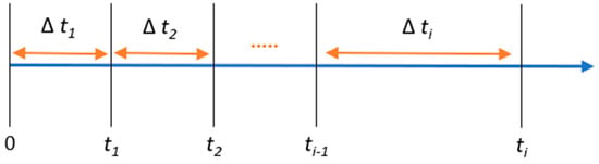
Figure 1. Software failure process [2].

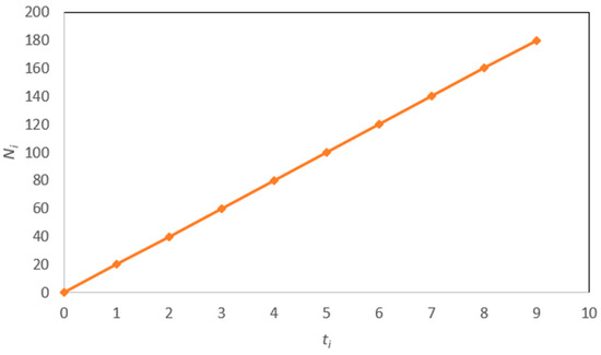
Figure 2. An example of software reliability data [2].

In this work, we adopted a deep learning approach and ensemble method for software reliability testing to enhance the reliability of critical computer vision systems. To the best of our knowledge, there is no prior research work that is dedicated to enhancing the performance of computer vision systems through software reliability testing.

This paper is organized as follows. Section 2 provides a review and discussion of the main works on deep learning-based software reliability prediction models. Section 3 explains the new model architecture and its design in detail. Section 4 presents the experimental evaluation, illustrating the model’s efficiency and accuracy. Finally, the conclusions are outlined in Section 5.

2. Related Works

In this section, we provide different deep learning-based models for software reliability prediction. In the literature, several deep learning models are proposed to predict errors and failures in software systems.

In [2], the authors built a software reliability prediction model using an ensemble of Feed-Forward Neural Networks (FFNNs). The combined model of multiple predictors could obtain higher software reliability prediction performance compared to single predictors.

An FFNN-based dynamic weighted combination model (PFFNN-DWCM) was proposed for software reliability prediction [3]. In order to build the PFFNN-DWCM model, four well-known SRGMs were integrated. Moreover, the authors proposed an RNN-based dynamic weighted combination model (PRNN-DWCM) to improve the accuracy of software reliability prediction.

In [5], an on-line adaptive software reliability prediction model using an evolutionary connectionist approach based on multiple-delayed-input single-output architecture was proposed. In the network training scheme, Bayesian regularization was applied to improve the generalization capability. An artificial neural network-based approach for software reliability estimation was proposed [6]. Then, a dynamic weighted combinational model (DWCM) was built using the neural network approach.

Fuzzy Wavelet Neural Network (FWNN-SRGM) was used to build a software reliability growth model [7]; they compared FWNN-SRGM with a Back-Propagation Neural Network based software reliability growth model (BPNN-SRGM). BPNN has difficulty in determining the network architecture; thus, phase space reconstruction technology and the FWNN were used to increase the prediction accuracy. A novel recurrent architecture for Genetic Programming (GP) and Group Method of Data Handling (GMDH) was proposed to predict software reliability [8].

In [9], a neural network combination model based on dynamically evaluated weights was proposed in order to improve the goodness of fit of the already proposed traditional SRGM and ANN-based combination models. In [10], the authors proposed an infinite test effort function in conjunction with a classical NHPP model and use an Artificial Neural Network (ANN) for training the proposed model.

A nonparametric method using a radial basis function neural network was proposed for predicting software reliability [11]. The Bayesian regularization method was applied in the proposed model to improve the generalization and to avoid the overfitting problem.

In [12], the authors employed an RNN encoder–decoder to estimate the number of failures. RNN was successfully used in sequence-to-sequence problems. An SRGM based on Pareto distribution (PD) and artificial FFNN was presented [13]. It is a novel software testing method used to find appropriate reliability models in software development. PD was utilized to estimate the distribution of faults within the software.

A software reliability prediction method for cross-project predictions was proposed [14]. For ongoing projects, the data may be limited or insufficient to accurately predict the number of failures. Therefore, the required data were obtained from related projects. The proposed model was built using deep LSTM for predicting the number of failures in the target project. In an ongoing phase with insufficient data, this method enables software developers and managers to better understand the state of the project.

In [15], the authors proposed a deep learning-based approach for software reliability prediction and assessment. Specifically, they demonstrated how to derive mathematical expressions from the computational methods of deep learning models and how to determine the correlation between them and the mathematical formula of SRGMs, and then, they used a back-propagation algorithm to obtain the SRGM parameters. Furthermore, they integrated some deep learning-based SRGMs, and also proposed a method for the weighted assignment of combinations.

To address the overfitting problem when using deep neural networks, the authors proposed the use of dropout [16]; this study utilized a deep learning model based on LSTM Encoder–Decoder Dropout to predict the number of faults in software and assess software reliability.

An attention-based encoder–decoder recurrent neural network was presented [17]; it was used for predicting the number of software failures. The incorporation of the attention technique enhanced the prediction accuracy within the encoder–decoder framework. In [18], the authors proposed a method of reliability assessment based on deep learning for open-source software (OSS). They investigated the difference between general data and specific data for the estimation of OSS reliability.

Predefined Artificial Intelligence algorithms, mainly Artificial Neural Network (ANN), Recurrent Neural Network (RNN), Gated Recurrent Unit (GRU) and Long Short-Term Memory (LSTM) were used for predicting software reliability [19].

A comparison was conducted between software reliability models that utilize NHPP and deep learning techniques [20]. The authors used a deep learning model based on recurrent neural networks and applied it to time-series data. The results indicated that the software reliability of the recurrent neural network model outperformed NHPP.

In [21], the authors proposed a hybrid long short-term memory (LSTM) with BrainStorm Optimization and the Late Acceptance Hill Climbing (BSO-LAHC) algorithm of a stepwise prediction model for software fault detection and correction.

A hybrid approach combining traditional statistical models (e.g., ARIMA) and deep learning techniques was proposed to improve software reliability predictions [22]. The integration leveraged ARIMA’s strengths in short-term pattern recognition and deep learning’s capacity for capturing complex, long-term dependencies.

The effectiveness of Automated Machine Learning (AutoML) in enhancing software reliability growth modeling was explored and its performance was compared with traditional SRGMs [23]. The authors employed two prominent AutoML packages, Auto-sklearn and H2O AutoML. In [24], the authors proposed several methods to enhance prediction accuracy in the software reliability context. More specifically, they introduced two gradient-based techniques for estimating the parameters of classical SRGMs and proposed methods involving LSTM encoder–decoder and Bayesian approximation within Langevin Gradient and Variational inference neural networks.

A comparative analysis of the deep learning-based software reliability prediction models is provided in Table 1.

Table 1. Comparative analysis of the deep learning-based software reliability prediction models.

The Model	The Used Neural Network	Model Type	No. of Datasets	The Metrics of Prediction Performance
[2] (2009)	Feed-forward Neural Network (FFNN)	Combined	2 datasets	Average relative error (AE) 1.2878 1.6339
[3] (2014)	Recurrent Neural Network (RNN)	Combined	3 datasets	Average relative error (AE) 1.1128 0.1069 0.1792
[7] (2010)	Fuzzy Wavelet Neural Network (FWNN)	Single	1 dataset	Mean square error (MSE) 0.04855
[10] (2017)	Feed-forward Neural Network (FFNN)	Single	4 datasets	Mean square error (MSE) 0.4823 0.4741 0.3485 0.4031
[12] (2018)	Recurrent Neural Network (RNN)	Single	14 datasets	Average Relative Error (AE) 0.02 Average bias (AB) + 0.02
[13] (2019)	Feed-forward neural network (FFNN)	Single	4 datasets	Mean square error (MSE) 0.414–0.426–0.225–1.546
[14] (2021)	Recurrent Neural Network (RNN)	Single	15 projects	Average Relative Error (AE) 0.110
[17] (2022)	Recurrent Neural Network (RNN)	Single	1 dataset	Mean square error (MSE) 0.50
[20] (2023)	Recurrent Neural Network (RNN)	Single	2 datasets	Mean square error (MSE) 2.1147 4.8223 Mean absolute error (MAE) 1.4127 2.0739

Based on Table 1, it can be observed that the models [2,10,13] used FFNN, while the models [3,12,14,17,20] used RNN. FWNN was used in [7]. The NN that was used in the prediction model affected the performance since some types of NN are more suitable to prediction tasks than the other types. RNN is suitable for speech recognition, handwriting and time series prediction tasks. It is used to model the sequential data in recognition and prediction tasks. It is known that there is no single SRGM that can achieve high prediction accuracy results in all cases. Thus, the combined model used in [2,3] was better than the single type used in [7,10,12,13,14,17,20]. In the work [2], the combined NN was compared with the single NN, and the combined NN had better performance than the single NN. The work [3] also compared the performance of the combined models, which consisted of four SRGMs with the models that were created by combining two or three SRGMs. The results showed that the combined model with four SRGMs consistently outperformed the models that were created by integrating two or three SRGMs. Both works [2,3] were combined, but [2] used FFNN while [3] used RNN, which is better in prediction tasks than FFNN. Moreover, in [3], a comparison was conducted between the RNN-based model and the FFNN-based model. The comparative results showed that the RNN obtained accurate predictive capability. In [12], the proposed model based on RNN was compared with FNN; the experimental results indicated that RNN performed better than FNN in terms of prediction accuracy.

The most important criterion in comparative analysis is the dataset. The performance and efficiency of a neural network model are significantly influenced by the characteristics of the handled datasets. The datasets that are used to evaluate the presented prediction models are different, and there is a different number of datasets for evaluating each model. Each dataset has a different data size and contains a different number of samples. Thus, the nature of a dataset affects the performance of an NN prediction model. We cannot determine the best performance or accurately compare the models based solely on the datasets used for evaluation. In [12], fourteen different datasets were used to evaluate the models. The datasets were collected from different domains such as a compiler project, a real-time command and control system, an online data entry control software package, a railway interlocking system and a flight dynamic application. In [13], the datasets were collected from the database of the Tandem computers company. In [14], fifteen different projects were obtained from the e-Seikatsu Co., Ltd. This is a Japan-based company that primarily provides cloud solutions to businesses. In [17], the dataset was obtained from a real-time control application containing roughly 870,000 code lines.

The performance metrics are Average Relative Error (AE) and Mean Square Error (MSE). AE was used to evaluate [2,3,12,14] while MSE was used in [7,10,13,17,20]. All metrics are used in predictive modeling to find the relation between the actual number of failures and the predicted number of failures obtained by the model but they use different equations. The difference is in the squared error, which is used in MSE. Therefore, AE is more robust to outliers since it does not rely on squaring errors. Conversely, MSE is beneficial if we focus on large errors, as it gives them greater weight compared to smaller ones. AE measures the model prediction performance for the whole testing phase, while the model bias is measured by AB. The predictive value is overestimated when AB is a positive while it is underestimated when AB is a negative. The model is consistent when the AE and AB values are equal; otherwise, it is inconsistent. Consistency means better stability. Based on the AE results, the RNN achieves higher accuracy, since the lower the AE, the higher its prediction accuracy.

Based on the comparison mentioned above, the combined RNN model was selected for use in the new proposed model. Prior works, such as [2,3], used combined neural network models without employing ensemble methods. However, the main contribution of this research is the adoption of an ensemble method for software reliability prediction, which proved to be a more accurate solution than a single model.

3. The Proposed Model Architecture and Its Detailed Design

In this section, we provide the proposed model architecture as shown in Figure 3. It has three phases: Preprocessing, Ensemble method and Prediction.

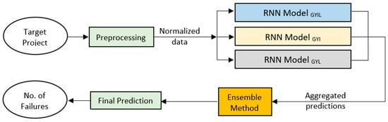
Figure 3. The proposed model architecture for software reliability testing.

3.1. Preprocessing

The failure dataset is split into two parts: the first part is utilized in the training phase to train the neural network. Then, the second part is used in the testing phase to evaluate the effectiveness and validity of the predictions when deployed in real-world applications. Thus, the trained neural network is utilized to predict the test set of the failure data. The predicted failure number is compared with the actual failure number from the dataset.

Before feeding the inputs into the model, execution time and number of failures are normalized to a range of [0, 1]. Normalization is a common preprocessing technique that adjusts the scale of numerical data while preserving the differences in the value ranges. It ensures that features with larger numerical ranges do not overly affect the model’s learning process compared to features with smaller ranges. First, for each input, the minimum and maximum values are identified from the dataset. These are denoted as $x_{min}$ and $x_{max}$, respectively. Then, each value $x_i$ of the feature is transformed using the formula [25]:

$$x_{normalized}={\displaystyle \frac{x_i-x_{min}}{x_{max}-x_{min}}},$$

(1)

this formula scales the values of the input within the range of [0, 1].

Many deep learning models perform better and converge faster when input features are on a similar scale. Normalization ensures consistent representation of the data, especially when combining features with vastly different units.

By normalizing the execution time and number of failures, the model can focus on learning the patterns in the data without being skewed by the magnitude of raw numerical values. This phase produces normalized data to be used as input for RNN models.

3.2. The Ensemble Method and Prediction

3.2.1. Software Reliability Model Architecture

RNNs are a class of neural networks specifically designed for sequential and time-dependent data [3,26,27]. Unlike traditional feedforward neural networks, which assume that all inputs are independent of each other, RNNs can process sequences of data by maintaining a “memory” of previous inputs through internal states. This makes RNNs particularly well-suited for tasks involving temporal patterns, such as time-series forecasting, language modeling, and speech recognition. The key features of RNNs are a feedback mechanism, dynamic temporal properties, and learning temporal dependencies.

In RNNs, the output of one timestep is fed back as input into the next timestep, alongside the new input. This feedback loop allows the network to incorporate historical context into its predictions. The internal states of the RNN evolve capturing temporal dynamics in the input sequence. These evolving states help the model remember earlier inputs and adjust their predictions dynamically based on new data. RNNs excel at learning patterns in sequential data, where the order and timing of inputs matter.

The advantages of the proposed RNN model include handling sequential data, capturing temporal patterns, having a flexible architecture, and making dynamic predictions.

The feedback mechanism allows the network to incorporate information from previous timesteps, enabling it to model dependencies over time. This is especially useful in datasets where past events influence future outcomes. The model’s internal states can adapt dynamically, enabling it to recognize patterns like delays, repetitions, or long-term trends in sequences. The proposed RNN model can handle variable-length sequences, making it robust for real-world applications where input lengths may differ. By incorporating feedback, the RNN can adjust its predictions dynamically as new inputs are provided, making it ideal for real-time applications like live translation or streaming data analysis.

The equation ${y″}_i=f\left({y″}_{i-1},t_i\right)$ is used to predict ${y″}_i$ using ${y″}_{i-1}$. Thus, the cumulative number of failures at time $t_i$ is considered as a function of the cumulative number of failures at time $t_{i-1}$ and the current execution time $t_i$. The RNN model is constructed using a feedback path from the output layer to the hidden layer through the recurrent neuron, labeled R, as shown in Figure 4. Therefore, it can identify the cumulative number of failures in execution time $t_{i-1}$. The input of the RNN model is the software execution time ($t_i$), while the output of the RNN model is the predicted cumulative number of software failures (${y″}_{i-1}$). The activation functions $1-e^{-x}$, $1-\left(1+x\right)e^{-x}$, $\left(1-e^{-x}\right)/\left(1+a_2{e}^{-x}\right)$ and $1/\left(1+b_2{e}^{-x}\right)$ are applied in the four hidden neurons. In the output layer, a linear activation function is used. The output of the RNN model is presented as follows [3]:

$$\begin{gathered} {y″}_i={w^{\prime }}_5\left(1-e^{-{w^{\prime }}_1{t}_i}\right)+{w^{\prime }}_6\left(1-\left(1+{w^{\prime }}_2{t}_i\right)e^{-{w^{\prime }}_2{t}_i}\right) \\ +{\displaystyle \frac{{w^{\prime }}_7\left(1-e^{-{w^{\prime }}_3{t}_i}\right)}{1+a_2{e}^{-{w^{\prime }}_3{t}_i}}}+{\displaystyle \frac{{w^{\prime }}_8}{1+b_2{e}^{-{w^{\prime }}_4{t}_i}}}+{w^{\prime }}_9{y^{″}}_{i-1}, \end{gathered}$$

(2)

where ${w^{\prime }}_9$ is the feedback weight, ${w^{\prime }}_j$ > 0, for j = 1, 2, …, 9 and $a_2$, $b_2$ > 0. The learning algorithm determines the values of all of the weights and parameters of the RNN model. This model is able to incorporate the cumulative number of failures from previous execution times, which significantly enhances its predictive capability.

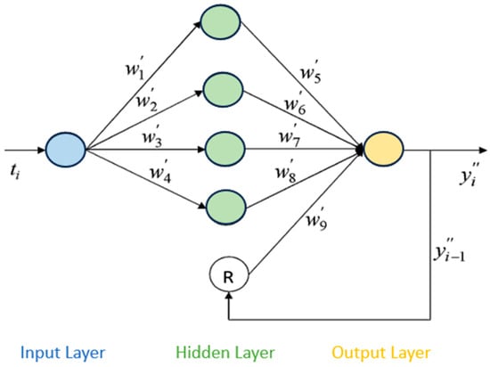
Figure 4. RNN architecture [3].

We proposed an RNN model that integrates the traditional SRGMs to create a software reliability model. We utilized four well-known traditional statistical SRGMs: the Goel–Okumoto model (G) [28], Yamada delayed s-shaped model (Y) [29], inflection s-shaped model (I) [30] and logistic growth curve model (L) [31,32]. Then, we built three RNN models. The first RNN model was created by integrating the four chosen SRGMs (GYIL). The second RNN model was created by integrating three of the four chosen SRGMs (GYI). The third RNN model was created by integrating three of the four chosen SRGMs (GYL). All of these models were trained using the normalized data generated during the preprocessing phase. Once the training of each RNN model was completed, an initial prediction was produced by each individual model. These initial predictions were then combined to create the aggregated predictions, which served as the input for the ensemble method phase.

3.2.2. Ensemble Method

It is known that no individual SRGM can consistently achieve accurate prediction results in all situations. An ensemble method is a machine learning technique that constructs multiple models and combines their outputs to improve the overall performance, accuracy, and robustness compared to a single model [33,34]. Therefore, we proposed to use ensemble methods as the main contribution of this research to improve software reliability testing. In this phase, we tested and evaluated different ensemble methods. There are various ensemble methods such as hard voting, soft voting, and stacking-based ensemble methods.

The aggregated predictions were utilized as input to generate the final prediction through the ensemble method. This method combines the outputs from multiple models, leveraging their collective strengths to enhance accuracy and reliability, ultimately producing a more robust final prediction.

The proposed RNN model architecture typically comprises multiple recurrent neural networks (RNNs) that are trained individually. These models are then integrated through an ensemble method to produce a final output. Each RNN in the ensemble is designed to process sequential data.

The proposed RNN model structure incorporates multiple individual RNNs, which are trained in parallel. Each RNN processes the same normalized input data but may focus on learning different patterns or features depending on the configuration. The RNN model has three layers: the input layer, the hidden layer and the output layer. The input layer processes normalized sequential data. The hidden layer within each RNN captures temporal dependencies and complex sequence patterns. Each RNN generates its own prediction through a dense layer followed by a softmax activation function. Then, the outputs of the individual RNNs are aggregated to be used as input for the ensemble method phase.

The main features of the proposed RNN model include training multiple RNNs in parallel, capturing diverse perspectives, and reducing the risk of overfitting to specific patterns in the data. The ensemble method improves generalization by combining the strengths of individual RNNs, leading to more robust predictions. Each RNN can be customized or fine-tuned independently, allowing for flexibility in addressing specific challenges in the data. The architecture can be scaled to include additional RNNs or variations to further enhance its performance.

This detailed architecture ensures the proposed RNN model is capable of handling complex, sequential data effectively.

Overall, the workflow can be summarized as follows:

• Input: Normalized data is fed into each RNN.
• Training: Each RNN learns to predict based on its architecture and training configuration.
• Initial Predictions: Individual RNN predictions are combined using an ensemble strategy.
• Final Output: The ensemble output serves as the final prediction, typically with improved accuracy and reliability.

4. Experimental Evaluation

In this section, we conducted two main experiments. In the first experiment, we introduced the experimental results of the proposed model for software reliability testing on public datasets. We conducted several experiments to test and evaluate different combined and ensemble methods such as hard voting, soft voting, and stacking-based ensemble methods. In the second experiment, we evaluated our new proposed model by conducting an experiment using a specific computer vision application in the security field to validate our contribution. Critical computer vision applications in the security field are essential for enhancing safety, monitoring environments, and automating the detection of potential threats. Therefore, we selected a face recognition system, which is one of the most popular computer vision applications in the security field. It is used in access control systems where face recognition technology identifies and verifies individuals to grant or deny access to secure areas.

4.1. Evaluation on Public Datasets

4.1.1. Datasets

We carry out the experiments using four datasets:

• Dataset 1 [20]: It is sourced from PLC4X, which is a collection of libraries designed for communication with industrial programmable logic controllers (PLCs). The data reflect the cumulative number of failures that occurred between December 2017 and January 2022.
• Dataset 2 [20]: It is derived from Apache Camel, which is an open-source integration framework that enables rapid and straightforward integration of different systems that consume or produce data. It contains data on the cumulative number of failures between April 2011 and January 2022.
• Dataset 3 [35]: It is collected by the Jet Propulsion Laboratory (JPL), part of NASA. It consists of 181 failure-count data points.
• Dataset 4 [35]: It is collected by JPL. It contains 73 failure-count data points.

All datasets used 80% of the data in the training phase. The other 20% of the data were utilized for the final evaluation.

4.1.2. Metrics

To evaluate the effectiveness of our proposed model, we leveraged two commonly used evaluation metrics: the mean squared error (MSE) and the mean absolute error (MAE). These two metrics are calculated as the sum of the squared distances and absolute values of the distances between the estimated and actual values, divided by the difference between the number of observations and parameters [36,37]:

$$MSE={\displaystyle \frac{{\sum }_{i=1}^n{\left(\widehat{m}\left(t_i\right)-y_i\right)}^2}{n-m}},$$

(3)

$$MAE={\displaystyle \frac{{\sum }_{i=1}^n\left|\widehat{m}\left(t_i\right)-y_i\right|}{n-m}}$$

(4)

4.1.3. Baselines

To demonstrate the efficiency of our proposed method, we compared it against three single RNN models [20] as baselines: recurrent neural networks (RNN), long short-term memory (LSTM), and gated recurrent units (GRU), which are the fundamental types of recurrent neural networks.

We mainly compared our proposed model to the single RNN models that have been applied to the same datasets (Dataset 1 [20] and Dataset 2 [20]) to ensure the fairness of the comparison.

4.1.4. Testing Set Results and Analysis

Table 2, Table 3, Table 4 and Table 5 show the experimental results of our proposed model compared to the other RNN models on Dataset 1, Dataset 2, Dataset 3, and Dataset 4, respectively. These experimental results were obtained from the testing set, which comprises 20% of the total dataset, and were used to evaluate the model’s performance on unseen data.

Table 2. The performance of our proposed model in comparison with single model results on Dataset 1.

Type	The Model	Dataset 1
		MSE	MAE
Single	RNN [20] (2023)	2.1147	1.4127
	LSTM [20] (2023)	2.0069	1.4104
	GRU [20] (2023)	2.0159	1.3983
Combined	Two RNN models	0.0054554534	0.0682218
	Three RNN models	0.000751277	0.019038694
Ensemble	Soft Voting	0.00019269866	0.012343713
	Hard Voting	0.00041984202	0.01657617
	Stacking	0.00037080966	0.016825633
(Our proposed model) Combined + Ensemble	SRGM-based RNN with Soft Voting	7.873888 × 10−5	0.0076218164
	SRGM-based RNN with Hard Voting	0.0075691612	0.08392381

Table 3. The performance of our proposed model in comparison with single model results on Dataset 2.

Type	The Model	Dataset 2
		MSE	MAE
Single	RNN [20] (2023)	4.8223	2.0739
	LSTM [20] (2023)	4.6712	2.0805
	GRU [20] (2023)	4.5494	2.0688
Combined	Two RNN models	0.032340303	0.16565005
	Three RNN models	0.023503931	0.14079273
Ensemble	Soft Voting	0.0164228	0.11144097
	Hard Voting	0.061417855	0.23531063
	Stacking	0.0115000	0.12866817
(Our proposed model) Combined + Ensemble	SRGM-based RNN with Soft Voting	0.0030255595	0.046620604
	SRGM-based RNN with Hard Voting	0.0030421042	0.048603985

Table 4. The performance of our proposed model in comparison with other model results on Dataset 3.

Table	The Model	Dataset 3
		MSE	MAE
Combined	Two RNN models	0.006116769	0.0690504
	Three RNN models	0.002586007	0. 043124218
Ensemble	Soft Voting	0.003776515	0.049680855
	Hard Voting	0.026597206	0.16071995
	Stacking	0.002558577	0.042795755
(Our proposed model) Combined + Ensemble	SRGM-based RNN with Soft Voting	0.001421848	0.026829486
	SRGM-based RNN with Hard Voting	0.004254901	0.036085066

Table 5. The performance of our proposed model in comparison with other model results on Dataset 4.

Type	The Model	Dataset 4
		MSE	MAE
Combined	Two RNN models	0.001227453	0.033979435
	Three RNN models	0.000297544	0.01542935
Ensemble	Soft Voting	0.000241060	0.013691017
	Hard Voting	0.5264526	0.72470796
	Stacking	0.000461192	0.01780403
(Our proposed model) Combined + Ensemble	SRGM-based RNN with Soft Voting	2.7830302 × 10−5	0.003663206
	SRGM-based RNN with Hard Voting	0.001330984	0.0231023007

Based on Table 2, Table 3, Table 4 and Table 5, it can be observed that the results of our proposed model with soft voting outperform other models, indicating the robustness and effectiveness of our model. The results show that the soft voting ensemble method obtains better results compared to other ensemble methods. Moreover, the combined model that uses three models outperforms the model that incorporates only two models, which indicates that combining more models can achieve more powerful predictive results.

Figure 5 and Figure 6 show the MSE and MAE results of our proposed model compared to other models on Dataset 1, Dataset 2, Dataset 3, and Dataset 4, respectively.

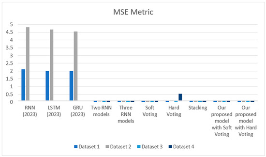
Figure 5. MSE results over the models.

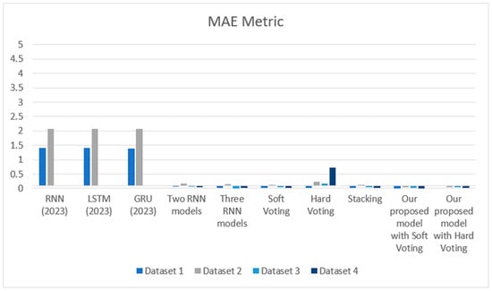
Figure 6. MAE results over the models.

4.1.5. Training Set Results and Analysis

Table 6 shows the results of our proposed model during the training phase. For all datasets, the MSE values indicate very small prediction errors on average. Thus, the proposed model captures the underlying pattern of the data quite well. The MAE values show that the model’s errors are consistent without significant outliers. R² measures the proportion of variance in the target variable explained by the model. R² values indicate that the model has excellent explanatory power and fits the data well. Overall, these results indicate that our proposed model performs exceptionally well, with low error metrics (MSE, MAE) and a high R² value, indicating strong predictive accuracy and a well-fitted model.

Table 6. The performance of our proposed model during the training phase.

Dataset	The Metric	The Result
Dataset 1	MSE	0.0008967413
	MAE	0.0246243632
	R2	0.9844007758
Dataset 2	MSE	0.0017010848
	MAE	0.0337057795
	R2	0.9745221365
Dataset 3	MSE	0.0045180714
	MAE	0.0535145577
	R2	0.9663832962
Dataset 4	MSE	0.0004653699
	MAE	0.0168053023
	R2	0.9924251697

Figure 7 shows the graphs that combine the actual and predicted values for the training data. The black lines represent the actual values, and the blue points are the predicted values.

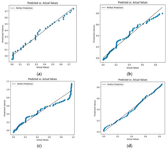
Figure 7. (a) Actual and predicted values for Dataset 1; (b) Actual and predicted values for Dataset 2; (c) Actual and predicted values for Dataset 3; (d) Actual and predicted values for Dataset 4.

Our proposed model can handle larger datasets and higher computational costs. It is able to maintain its level of performance. Scalability can be addressed across various strategies, such as scaling up the model’s capacity by increasing the number of layers or neurons. Also, using regularization techniques such as dropout, weight decay, or batch normalization can avoid overfitting. To handle large datasets effectively, strategies can be used to optimize storage, processing speed, memory usage, and training efficiency. To optimize data storage, efficient file formats can be used, such as TFRecords (TensorFlow), HDF5, or LMDB. These formats reduce storage space and improve data access speed compared to plain text or CSV files. For memory usage efficiency, data generators are used to load data batch-by-batch on the fly, reducing memory overhead. For training optimization, the proposed model can be tested on smaller dataset subsets to identify issues in architecture or hyperparameters before scaling up to the full dataset. Moreover, validation metrics can be monitored to stop training when performance plateaus to save resources. To speed up the training process, GPUs/TPUs are used. As in the transfer learning technique, our pre-trained model can be used to fine-tune it on the larger dataset instead of training from scratch. Knowledge distillation can be used to reduce memory and inference latency.

The computational cost of our proposed model depends on several factors such as the model’s complexity, dataset size, hardware, and the training process. Model complexity depends on the number of parameters and the depth of the model, since more parameters and deeper models require more computation, increasing the cost. Our proposed model has three layers and requires fewer parameters. The size of the model’s input affects computation; the inputs of our proposed model are small sequences of numbers, requiring fewer computations. The size of the datasets needs a few epochs, decreasing the total computation time. During the training process, we used a small batch size and a limited number of epochs. Small batch sizes require less memory and computational power per step. The small number of training iterations also minimizes the cost. Early stopping is used to reduce the computational cost by terminating training when the validation loss stops improving for 10 consecutive epochs. We used GPUs and TPUs to reduce the actual computational time and energy consumption.

To estimate the computational cost, the time and number of Floating Point Operations (FLOPS) can be measured for a forward pass and backward pass of our proposed model. Also, the inference time can be measured, along with the training time and memory requirements, including model weights and intermediate activations. To manage and reduce these computational costs, model optimization techniques can be used, such as pruning, quantization, knowledge distillation, and efficient architectures.

4.2. Evaluation on Face Recognition Dataset

4.2.1. Face Recognition Model

In this experiment, we utilized DeepFace, which is an open-source face recognition system. It has several deep learning models (e.g., VGG-Face, Google FaceNet, OpenFace).

4.2.2. Face Recognition Dataset

There are various well-known benchmark datasets commonly used for face recognition tasks, which differ in terms of size and complexity. In this experiment, we used the Labeled Faces in the Wild (LFW) dataset, which is one of the most used face recognition datasets. It contains 13,000 labeled images of faces from the internet, with 1680 individuals having two or more different images. It is designed for face verification and face recognition. It is widely used for benchmarking algorithms that determine whether two face images belong to the same person or not. It includes several challenges, such as natural variations in pose, lighting, background, and expression. The images are directly copied from the original LFW dataset, preserving their original size and color format. We selected randomly 200 individuals who have at least three images.

4.2.3. Face Recognition Failures

In face recognition systems, several types of failures can occur, each arising from different stages of the process such as face detection, alignment, feature extraction, or recognition. We considered the most common type of failure, which is False Negatives (False Rejection). In this failure, the system fails to recognize a known person. This may be caused by variations in appearance (e.g., makeup, glasses, aging), environmental factors (e.g., lighting, angle), or insufficient data during training. This failure causes frustration for legitimate users and leads to a poor user experience.

4.2.4. Results

We used the face recognition models in DeepFace and the LFW dataset to build the dataset of the software failure data. This dataset contains the cumulative number of face recognition system failures as shown in Table 7.

Table 7. Cumulative number of face recognition system failures.

Index	Failures	Cumulative Failures	Index	Failures	Cumulative Failures
1	0	0	37	0	77
2	2	2	38	2	79
3	3	5	39	2	81
4	3	8	40	0	81
5	3	11	41	0	81
6	2	13	42	0	81
7	3	16	43	2	83
8	3	19	44	0	83
9	3	22	45	0	83
10	3	25	46	0	83
11	3	28	47	0	83
12	3	31	48	2	85
13	2	33	49	0	85
14	0	33	50	1	86
15	0	33	51	0	86
16	0	33	52	3	89
17	0	33	53	3	92
18	0	33	54	3	95
19	3	36	55	3	98
20	3	39	56	3	101
21	1	40	57	3	104
22	0	40	58	3	107
23	1	41	59	3	110
24	1	42	60	3	113
25	3	45	61	3	116
26	3	48	62	2	118
27	2	50	63	0	118
28	3	53	64	1	119
29	3	56	65	0	119
30	3	59	66	1	120
31	3	62	67	2	122
32	3	65	68	3	125
33	3	68	69	3	128
34	3	71	70	3	131
35	3	74	71	3	134
36	3	77	72	2	136

After building the face recognition system failures dataset, we evaluated our new proposed model on this dataset. The experimental results were derived from the testing set, which represents 20% of the entire dataset, and served to assess the model’s performance on previously unseen data. The results of MSE and MAE were 0.00019184346 and 0.011849007, respectively. These experimental results validated our contribution and indicate the high accuracy and effectiveness of our proposed model; it achieves low MSE and MAE, which signifies that the model can effectively predict the reliability of software systems.

4.3. The Cross-Validation Results

Cross-validation is a statistical method used to evaluate and compare the performance of deep learning models by dividing data into subsets (training and validation) multiple times. Instead of training and evaluating the model on a single split, cross-validation systematically evaluates the model across several splits to reduce the risk of overfitting and underfitting. There are several types of cross-validation, such as K-Fold Cross-Validation, Stratified K-Fold, Leave-One-Out Cross-Validation (LOOCV), and Repeated K-Fold. In this experiment, we employed K-Fold Cross-Validation, which divides the dataset into k equal folds and performs k iterations.

We utilized the cross-validation method to provide a more reliable estimate of our proposed model’s performance by testing it on multiple validation sets and validating the model’s ability to generalize to new data, avoiding overfitting to the training set. Also, this reduced the risk of bias introduced by a single train-test split and allowed the calculation of average metrics across all folds for a robust evaluation. Cross-validation makes efficient use of a dataset by rotating the training and validation data, especially when the dataset is small. In Table 8, the cross-validation results indicate the robustness of our proposed model.

Table 8. The cross-validation results.

Dataset	MSE	MAE
Dataset 1	0.001200671	0.027496923
Dataset 2	0.004177866	0.047704391
Dataset 3	0.011405760	0.087417414
Dataset 4	0.002694746	0.035844000
Face recognition dataset	0.001203766	0.028293835

5. Conclusions and Future Work

In this paper, we propose a new model that uses a combined RNN model, which is better for prediction tasks. Moreover, the proposed model uses the ensemble method to improve predictive capability and hence enhance performance. This model is the first software reliability model that includes combined and ensemble methods. The main objective of this research was to improve the performance of software reliability testing for computer vision systems and to deliver error-free and high-quality products to users according to their requirements. We believe that our proposed model will assist software developers in predicting software failures during the development and testing phases to minimize failures and improve overall software quality.

The experimental results showed that the proposed model can accurately predict the number of software failures. It had higher predictive accuracy for software reliability compared to other single neural network-based software reliability models. In the future, we plan to expand our research by utilizing optimization methods, such as genetic algorithms or reinforcement learning, to enhance the performance and efficiency of the current approach. These techniques could provide novel solutions to improve parameter tuning, decision-making processes, or adaptability to complex scenarios, offering a more robust and scalable framework.

Moreover, future work will involve evaluating other critical computer vision applications and extending the proposed methods using more diverse and representative datasets from various software domains and computer vision tasks such as PLC4X, Apache Camel, and LFW. This will help to assess and improve the scalability, robustness, and generalization of our proposed model, ensuring its applicability in real-world scenarios across multiple fields.

References

- Musa, J.D. Software Reliability Engineering: More Reliable Software, Faster and Cheaper; Tata McGraw-Hill Education: New York, NY, USA, 2004. [Google Scholar]
- Zheng, J. Predicting software reliability with neural network ensembles. Expert Syst. Appl. 2009, 36, 2116–2122. [Google Scholar] [CrossRef]
- Roy, P.; Mahapatra, G.; Rani, P.; Pandey, S.; Dey, K. Robust feedforward and recurrent neural network based dynamic weighted combination models for software reliability prediction. Appl. Soft Comput. 2014, 22, 629–637. [Google Scholar] [CrossRef]
- Li, S.; Yin, Q.; Guo, P.; Lyu, M.R. A hierarchical mixture model for software reliability prediction. Appl. Math. Comput. 2007, 185, 1120–1130. [Google Scholar] [CrossRef]
- Tian, L.; Noore, A. On-line prediction of software reliability using an evolutionary connectionist model. J. Syst. Softw. 2005, 77, 173–180. [Google Scholar] [CrossRef]
- Su, Y.-S.; Huang, C.-Y. Neural-network-based approaches for software reliability estimation using dynamic weighted combinational models. J. Syst. Softw. 2007, 80, 606–615. [Google Scholar] [CrossRef]
- Zhao, L.; Zhang, J.-P.; Yang, J.; Chu, Y. Software reliability growth model based on fuzzy wavelet neural network. In Proceedings of the 2010 2nd International Conference on Future Computer and Communication, Wuhan, China, 21–24 May 2010; IEEE: Piscataway, NJ, USA, 2010; Volume 1. [Google Scholar] [CrossRef]
- Mohanty, R.; Ravi, V.; Patra, M. Hybrid intelligent systems for predicting software reliability. Appl. Soft Comput. 2013, 13, 189–200. [Google Scholar] [CrossRef]
- Lakshmanan, I.; Ramasamy, S. An artificial neural-network approach to software reliability growth modeling. Procedia Comput. Sci. 2015, 57, 695–702. [Google Scholar] [CrossRef]
- Ramasamy, S.; Lakshmanan, I. Machine learning approach for software reliability growth modeling with infinite testing effort function. Math. Probl. Eng. 2017, 2017, 8040346. [Google Scholar] [CrossRef]
- Bal, P.R.; Mohapatra, D.P. Software reliability prediction based on radial basis function neural network. In Advances in Computational Intelligence: Proceedings of International Conference on Computational Intelligence 2015; Springer: Singapore, 2017. [Google Scholar] [CrossRef]
- Wang, J.; Zhang, C. Software reliability prediction using a deep learning model based on the RNN encoder decoder. Reliab. Eng. Syst. Saf. 2018, 170, 73–82. [Google Scholar] [CrossRef]
- Sudharson, D.; Prabha, D. A novel machine learning approach for software reliability growth modelling with pareto distribution function. Soft Comput. 2019, 23, 8379–8387. [Google Scholar] [CrossRef]
- San, K.K.; Washizaki, H.; Fukazawa, Y.; Honda, K.; Taga, M.; Matsuzaki, A. Deep cross-project software reliability growth model using project similarity-based clustering. Mathematics 2021, 9, 2945. [Google Scholar] [CrossRef]
- Wu, C.-Y.; Huang, C.-Y. A study of incorporation of deep learning into software reliability modeling and assessment. IEEE Trans. Reliab. 2021, 70, 1621–1640. [Google Scholar] [CrossRef]
- Oveisi, S.; Moeini, A.; Mirzaei, S. LSTM Encoder-Decoder Dropout Model in Software Reliability Prediction. Int. J. Reliab. Risk Saf. Theory Appl. 2021, 4, 1–12. [Google Scholar] [CrossRef]
- Li, C.; Zheng, J.; Okamura, H.; Dohi, T. Software reliability prediction through encoder-decoder recurrent neural networks. Int. J. Math. Eng. Manag. Sci. 2022, 7, 325. [Google Scholar] [CrossRef]
- Miyamoto, S.; Tamura, Y.; Yamada, S. Reliability assessment tool based on deep learning and data preprocessing for OSS. Am. J. Oper. Res. 2022, 12, 111–125. [Google Scholar] [CrossRef]
- Jindal, A.; Gupta, A. Comparative Analysis of Software Reliability Prediction Using Machine Learning and Deep Learning. In Proceedings of the 2022 Second International Conference on Artificial Intelligence and Smart Energy (ICAIS), Coimbatore, India, 23–25 February 2022; IEEE: Piscataway, NJ, USA, 2022. [Google Scholar] [CrossRef]
- Kim, Y.S.; Song, K.Y.; Chang, I.H. Prediction and Comparative Analysis of Software Reliability Model Based on NHPP and Deep Learning. Appl. Sci. 2023, 13, 6730. [Google Scholar] [CrossRef]
- Raamesh, L.; Jothi, S.; Radhika, S. Enhancing software reliability and fault detection using hybrid brainstorm optimization-based LSTM model. IETE J. Res. 2023, 69, 8789–8803. [Google Scholar] [CrossRef]
- Samal, U.; Kumar, A. Enhancing software reliability forecasting through a hybrid ARIMA-ANN model. Arab. J. Sci. Eng. 2024, 49, 7571–7584. [Google Scholar] [CrossRef]
- Kim, T.; Ryu, D.; Baik, J. Automated Machine Learning for Enhanced Software Reliability Growth Modeling: A Comparative Analysis with Traditional SRGMs. In Proceedings of the 2024 IEEE 24th International Conference on Software Quality, Reliability and Security (QRS), Cambridge, UK, 1–5 July 2024. [Google Scholar] [CrossRef]
- Oveisi, S.; Moeini, A.; Mirzaei, S.; Farsi, M.A. Software reliability prediction: A machine learning and approximation Bayesian inference approach. Qual. Reliab. Eng. Int. 2024, 40, 4004–4037. [Google Scholar] [CrossRef]
- James, G.; Witten, D.; Hastie, T.; Tibshirani, R.; Taylor, J. An Introduction to Statistical Learning: With Applications in R; Springer: Dordrecht, The Netherlands, 2013. [Google Scholar] [CrossRef]
- Goodfellow, I.; Bengio, Y.; Courville, A. Deep Learning; MIT Press: Cambridge, MA, USA, 2016. [Google Scholar]
- Shiva Prakash, B.; Sanjeev, K.V.; Prakash, R.; Chandrasekaran, K. A survey on recurrent neural network architectures for sequential learning. In Soft Computing for Problem Solving: SocProS 2017; Springer: Singapore, 2019; Volume 2. [Google Scholar] [CrossRef]
- Goel, A.L.; Okumoto, K. Time-dependent error-detection rate model for software reliability and other performance measures. IEEE Trans. Reliab. 1979, 28, 206–211. [Google Scholar] [CrossRef]
- Yamada, S.; Ohba, M.; Osaki, S. S-shaped software reliability growth models and their applications. IEEE Trans. Reliab. 1984, 33, 289–292. [Google Scholar] [CrossRef]
- Ohba, M. Inflection S-shaped software reliability growth model. In Stochastic Models in Reliability Theory, Proceedings of the Symposium Held in Nagoya, Japan, 23–24 April 1984; Springer: Berlin/Heidelberg, Germany, 1984. [Google Scholar] [CrossRef]
- Peleg, M.; Corradini, M.G.; Normand, M.D. The logistic (Verhulst) model for sigmoid microbial growth curves revisited. Food Res. Int. 2007, 40, 808–818. [Google Scholar] [CrossRef]
- Haque, A.; Ahmad, N. A logistic growth model for software reliability estimation considering uncertain factors. Int. J. Reliab. Qual. Saf. Eng. 2021, 28, 2150032. [Google Scholar] [CrossRef]
- Kunapuli, G. Ensemble Methods for Machine Learning; Simon and Schuster: New York, NY, USA, 2023. [Google Scholar]
- Sagi, O.; Rokach, L. Ensemble learning: A survey. Wiley Interdiscip. Rev. Data Min. Knowl. Discov. 2018, 8, e1249. [Google Scholar] [CrossRef]
- Lyu, M.R. Handbook of Software Reliability Engineering; IEEE Computer Society Press: Los Alamitos, CA, USA, 1996; Volume 222. [Google Scholar]
- Inoue, S.; Yamada, S. Discrete software reliability assessment with discretized NHPP models. Comput. Math. Appl. 2006, 51, 161–170. [Google Scholar] [CrossRef]
- Askari, R.; Sebt, M.V.; Amjadian, A. Askari, R.; Sebt, M.V.; Amjadian, A. A Multi-Product EPQ Model for Defective Production and Inspection with Single Machine, and Operational Constraints: Stochastic Programming Approach. In Logistics and Supply Chain Management. LSCM 2020; Communications in Computer and Information, Science; Molamohamadi, Z., Tirkolaee, E.B., Mirzazadeh, A., Weber, G.W., Eds.; Springer: Cham, Switzerland, 2021; Volume 1458. [Google Scholar] [CrossRef]
Disclaimer/Publisher’s Note: The statements, opinions and data contained in all publications are solely those of the individual author(s) and contributor(s) and not of MDPI and/or the editor(s). MDPI and/or the editor(s) disclaim responsibility for any injury to people or property resulting from any ideas, methods, instructions or products referred to in the content. |
© 2024 by the authors. Licensee MDPI, Basel, Switzerland. This article is an open access article distributed under the terms and conditions of the Creative Commons Attribution (CC BY) license (https://creativecommons.org/licenses/by/4.0/).