Abstract
Wood supply chains are complex, involving many stakeholders, intricate processes, and logistical challenges to ensure the timely and accurate delivery of wood products to customers. Weather-related variations in forest road accessibility further complicate operations. This paper explores the challenges faced by forest managers in targeting many delivery requirements—four or more. To address this, simulation-based optimization, using NSGA-III, a many-objective optimization algorithm, is proposed to simultaneously optimize often conflicting objectives primarily by minimizing delivery lead time, delivery deviations in backlogs, and delivery variation. NSGA-III enables the exploration of a diverse set of Pareto-optimal solutions that show trade-offs across a flexible set of four, or more, delivery objectives. A Discrete Event Simulation model is integrated to evaluate objectives in a complex wood supply chain. The implementation of NSGA-III within the framework allows forestry decision-makers to navigate between different harvest schedules and evaluate how they target a set of preference-based delivery objectives. The simulation can also provide detailed insights into how a specific harvest schedule affects the supply chain when post-processing possible solutions, facilitating decision making. This study shows that NSGA-III could substitute NSGA-II to optimize the wood supply chain for more than three objective functions.
1. Introduction
1.1. Problem
About half of Sweden is covered by forests. The products harvested annually amount to about 70.3 million m3 (2024) solid under bark and play an important role in the development of bio-based products. Wood deliveries begin with harvesting. Forest managers are responsible for scheduling harvesting to ensure the timely delivery of high-quality wood products to customers from hundreds of remote, geographically scattered harvesting sites. Wood deliveries to customers should be smooth with minimal variations and short lead times. To ensure smooth monthly wood flows from the harvest sites to different customers, the harvesting must be scheduled based on customer requirements and access to forest roads [1].
The harvest scheduling is handled by forest managers, using their experience and tools such as GIS software, but most of the planning is still undertaken manually [1]. In addition, to ensure the timely delivery of fresh wood to customers, landings at roadsides must be accessible for trucks to collect the wood immediately after harvesting operations. Road accessibility [2] is often critical and increasingly affected by climate change [3,4,5], as it depends on the physical condition of the roads [2]. For example, periods of thawing or heavy rainfall can significantly reduce road accessibility, which is crucial for deliveries. These factors must be considered in the scheduling process.
The number of delivery targets, or objectives, can vary considerably—but they tend to include product lead time or the on-time delivery of product volumes. Together, these objectives define a multi-objective problem. When objectives are evaluated for each product (for example, across multiple wood products), the problem expands and the number of objectives increases, turning it into a many-objective problem. Such problems require solution methods that go beyond those used for multi-objective optimization (MOO). In general, MOO deals with problems involving two to three objectives, whereas many-objective problems involve four or more objectives and thus demand different solution strategies. An experienced forest manager may also face the challenge of scheduling harvesting for multiple simultaneous delivery objectives as effectively as possible, while considering weather-dependent road accessibility. With decades of experience, managers solve an MOO problem without advanced proprietary tools or models to handle multi-objectives, which is further complicated by uncertainties such as weather [1] and landing accessibility in a production environment.
The harvesting problem to be solved includes at least two objectives: delivering products on time and ensuring short lead times. The customers are often large mills that require steady wood deliveries with consistent quality with fluctuations kept to a minimum. There are two delivery targets: to limit backlogs (wood not delivered) and delivery variations. More objectives could be of interest, for example, product-wise or otherwise, depending on the manager’s preferences. The need for multi-objective decision support is emphasized by Acuna et al. [6], preferably where the number and types of objectives are allowed to vary depending on preferences.
Multi-objective meta-heuristic optimization methods, which provide “good enough” solutions, are used in a variety of fields to solve optimization problems involving multiple objectives [7]. In particular, NSGA-II [8] is widely used for scheduling problems, as it can provide solutions for complex scheduling tasks [9], especially combinatorial scheduling problems [10], such as the harvest scheduling problem. Meta-heuristic evolutionary algorithms belong to the category of genetic algorithms (GAs), in which a set of solutions is iteratively improved through the simulation of evolution. This is achieved by combining parent solutions to produce new, improved child solutions using the operators’ crossover and mutation to search for improved solutions [8,11]. GAs, and particularly the Non-Dominated Sorting Genetic Algorithm II (NSGA-II) [8], have been used in a considerable number of scheduling problems to solve problems with multiple simultaneous objectives [9]. However, a limited number of papers address many-objective scheduling problems [9]. One possible reason is that genetic algorithms for multiple-objective optimization are known to be computationally demanding [12]. To the best of our knowledge, there are even fewer applications of many-objective optimization for harvest scheduling.
Harvest scheduling is a combinatorial MOO problem, scheduling harvest sites as a sequence to be harvested [1], which constitutes the decision variable. The scheduling should ensure short lead time (in days) and no delivery variation or product backlog (in cubic meters) [13], which are common delivery objectives and the least common denominator for most supply chains [14]. However, additional objectives turn the problem into a many-objective problem (with more than three objectives) and increase its complexity. Harvest scheduling should be able to handle any number of objectives to optimize delivery performance (DeP) to accommodate managers’ preferences while considering road accessibility to landings as a parameter. This requires methods that meet many objectives in MOO. This study aims to investigate methods for handling multiple objectives in the harvest scheduling problem [13] by applying NSGA-III instead of NSGA-II, to optimize harvest scheduling for additional objectives, and to propose a computational strategy for faster processing in a production environment.
1.2. Literature Review
Customers’ monthly and total annual demands are known in advance. Pulp and paper mills expect steady flows of the demanded product quality to maintain smooth production, and deliveries are expected to vary as little as possible to keep an even production pace. Sometimes, bonuses and penalties are included in delivery quotas to ensure deliveries are smooth and maintain expected inventory levels in the industry, minimizing the risk of backlogs, which can cause costly mill stops.
Harvest scheduling by sequencing the sites is established by a forest manager before harvesting to meet the demand of the customers for various wood products [15]. Harvesting is accomplished by teams, including a harvester and at least one forwarder, working in parallel according to the harvesting schedule. At each stand, trees with different stem diameters and product characteristics are bucked according to customers’ demand for optimized product specifications [16]. The forwarder transports and sorts the products in piles (buffers) at roadside landings to be transported by truck to saw or pulp mill customers. Weather fluctuations can make forest roads inaccessible [3,4], affecting deliveries [5]. The schedule should account for the weather-dependent accessibility of landings at harvest sites by matching the harvest time with the accessibility of the forest road [13]. Large volumes of wood at landings enable smoother wood flows by providing greater flexibility in transportation. Product quality is affected by lead time [17,18], where the majority of the time is storage in landings. Long lead times can negatively affect the quality of the wood, leading to quality loss and degradation [17,18]. At the same time, customer-specific products in landings awaiting transport to the customer also incur a cost. A side effect occurs when product volumes in that segment are insufficient, leading to overdelivery in the degraded segment. To maintain quality, the trucks strive to start customer deliveries as soon as possible, minimize delivery variations, and limit the risk of long lead times at roadside landings.
DeP indicators are vital to measure and evaluate supply chain performance of, e.g., timely and accurate deliveries [19]. Gunasekaran et al. [20] define several supply chain DeP metrics, such as delivery lead time, quality, and on-time deliveries, which have been identified as highly rated DeP objectives for a supply chain [14]. This aligns with the basic and common performance objectives of the wood supply chain: deliveries should be on time to reduce backlogs, backlogs should vary as little as possible, and the lead time should be as short as possible [17,18]. These objectives should therefore be minimized.
Westlund et al. [13] use a simulation-based multi-objective optimization (SMO) framework to compute Pareto-optimal harvest schedules for delivery objectives: lead time, on-time deliveries, and product throughput. The Pareto-front solutions offer a set of harvest schedules, allowing a decision-maker to determine the best solution based on trade-offs across the objectives: in this example, lead time versus delivery precision. Deriving DeP objective functions mathematically from a harvest schedule is a challenging task, because it involves all processes, from harvest to delivery, that affect performance and are therefore simulated in a DES [13]. To understand complex supply chains with numerous interdependencies and variables, Discrete Event Simulation (DES) is commonly used to evaluate delivery objectives, and is widely used to simulate different types of biomass and WSCs [21]. It can simulate system behavior to collect outputs for various system inputs and effectively capture DeP objectives for many-objective optimization problems.
In addition to varying road accessibility in the harvest scheduling problem, wood deliveries can also vary over time. To handle wood supply chain variations, different approaches are suggested to achieve more robust solutions [22,23,24]. Delivery variations should be reduced to ensure smooth delivery flows. Hopp [25] (Chapter 1) and Pound et al. [26] (Chapter 3) propose the Coefficient of Variation (CoV), dividing the standard deviation by the mean, as a measure of variability. Sanchez and Sanchez [27] suggests a quadratic loss function (scaled loss), , to capture variations by measuring the deviation from the target value for an output Y from a given input x (or solution). Westlund and Ng [28] adapts this loss objective function [27] for monthly back orders in the SMO framework for harvest scheduling. To capture both the mean annual product backlogs and their variations, such a loss objective could account for these fluctuations. Although not having backlogs is ideal, their variation should at least be less than the mean variation. An additional CoV objective could help control product-wise backlog variations. The SMO framework used in Westlund et al. [13] and Westlund and Ng [28] applies NSGA-II [8] to solve and schedule three to four performance objectives for the delivery, producing a set of Pareto-optimal harvest schedules. NSGA-II [8] is well suited for this problem when there are about four objectives [8]. Despite this effective implementation of finding Pareto-optimal solutions for harvesting scheduling [13], NSGA-II limits the number of objective functions in the scheduling.
To handle many objectives, such as sequential to NSGA-II [8], NSGA-III [11] is more effective in finding optimal and robust Pareto-optimal harvest scheduling solutions across 4 to 15 objectives. Compared to NSGA-II, NSGA-III requires predefined reference directions [11] to guide the search for Pareto solutions and identify a front with good spread and diversity, which increases computational effort.
Regardless of which meta-heuristic genetic algorithm is used, a multi-objective approach has previously been difficult to implement in business-oriented software. A bottleneck is that such simulation-based optimization approaches can be computationally intensive. This is particularly true when using GAs, where increasing population and generation sizes within the method directly increase the time required to generate the Pareto front. A population is a set of solutions, and each generation iteratively evaluates them to find better ones. Fitness evaluations in a genetic multi-objective approach, such as the meta-heuristic algorithms NSGA-II [8] and NSGA-III [11], can be both time and memory consuming [29], particularly for many objectives with many reference directions, and when the number of iterations of fitness evaluation grows.
For practical applications of NSGA-II/III, faster computation is required. Approaches to speed up calculations for practitioners are presented in Talbi et al. [12]. Both Talbi et al. [12] and Neumann et al. [30] discuss the benefits of distributed computing and parallel processing, which perfectly align with the structure of GAs, making it possible to iterate in parallel over solution populations and generations. Talbi et al. [12] exemplify different ways to make the meta-heuristic search process more efficient by leveraging parallelization on a distributed architecture. The iterative solution search in NSGA-II and NSGA-III is suitable for independent parallel evaluation within each generation [31], calculating individual solutions on different workers such as cores, computers, etc. Neumann et al. [30] also discusses the possibilities with cloud computing that provides scalable computational power as on-demand resources, which opens up new possibilities for companies to simplify the adaptation of the GAs in a production environment.
Today, there are several opportunities for companies to temporarily hire powerful computing capacity tailored to specific needs as a scalable, on-demand, self-service resource. It requires fewer resources, less expertise, and enables one to run computationally demanding models. Pătrăușanu et al. [31] analyzes five existing platforms for GA implementation, including the Python package pymoo [32]. They concluded that pymoo [32] is a generic platform capable of solving a wide range of problems, although performance varies depending on the type of problem. Pymoo is open-source software that adapts its algorithms to specific problems through an object-oriented design. The ability to customize and switch between algorithms is both straightforward and advantageous when evaluating their performance and suitability for real-world problems. However, the problem formulation and its associated operators (such as crossover and mutation) must be tailored to the specific problem, where Westlund et al. [13] suggest such operator customization effective for the harvest scheduling problem.
This study proposes an improved SMO framework [13,28] in two ways. First, NSGA-II is replaced with NSGA-III to more effectively handle optimization problems with more than four DeP objectives. In this study, these objectives include lead time, annual backlogs, volume-weighted backlog variations (to reduce total delivery variation over a year), and volume-weighted CoV. In addition, product-weighted CoV is included to minimize variance relative to the mean backlog and to enable comparison with the loss function. Since MOO algorithms are known to be computationally demanding [12], an efficient computational strategy is required to accelerate the optimization process. Second, we propose a modern solution based on renting on-demand computational resources to implement both NSGA-II and NSGA-III, thereby enabling faster computations and making the approach applicable in real-world applications.
2. Framework and Methods
2.1. Problem Formulation
Harvest scheduling is an MOO problem that aims to ensure robust deliveries with minimal lead time while remaining flexible to other objectives. This study is based on the SMO framework for harvest scheduling by Westlund et al. [13], which is based on NSGA-II for a multi-objective problem. The present research aims to extend the existing SMO framework tailored for DeP objectives to apply NSGA-III [11] to address many objectives. The two algorithms, NSGA-II and NSGA-III, are customized for the harvest scheduling problem to address the four DeP objectives in this study: lead time (LT), annual backlog (BL), a backlog loss function (loss BL) to minimize delivery variations for accumulated monthly backlogs for a year, and the Coefficient of Variation () for accumulated monthly backlogs for a year. Four objectives are chosen to benchmark and compare the methods, representing the upper limit of adequate performance for NSGA-II and the lower threshold of efficiency for NSGA-III. NSGA-II performs effectively with up to three to four objectives, while NSGA-III demonstrates efficient performance starting with four objectives and beyond. The study first customizes NSGA-III [11] using the Python package pymoo [32] for the combinatorial harvest scheduling problem. This includes calculating feasible directions for NSGA-III [11] to find a Pareto front with diversity and spread. The genetic operators proposed in Westlund et al. [13] are used for both methods.
The forest manager’s task is to schedule and evaluate the best trade-off among competing objectives, and decision-makers are interested in the practical application of the SMO framework. It is valuable to elaborate on the details of what happens in the WSC when a harvest schedule solution is applied. Accepting the trade-offs among objectives, a manager should also be able to obtain more detailed answers about what happens in the WSC when applying a solution. How lead time evolves and how backlogs change over time for different products are examples of such output variables. For this purpose, simulating a schedule in the DES, combined with visualizing results for decision support in a customized dashboard, can provide more details of a single harvesting solution. This approach is implemented in the study. Therefore, harvest schedules generated by the two methods are compared to analyze and compare DeP for similar solutions on the Pareto front. To align with a practical forest-industrial application, the SMO implementation is parallelized by using on-demand cloud computing via Microsoft Azure to accelerate calculations. Both NSGA-II and NSGA-III are implemented in Python (version 3.12.3) to run in parallel, further enhancing computational efficiency.
2.2. Simulation-Based Multi-Objective Optimization
Within such an SMO framework, a DES model for a WSC is integrated with an MOO algorithm to evaluate the DeP objectives of harvest schedules, while weather-dependent road accessibility is also handled as an input weather scenario, as described in Westlund et al. [13]. Hence, DES and MOO are tightly integrated, as shown in Figure 1, and implemented using the DES software FACTS Analyzer [33], which provides an Open API to interface with the Python program. The MOO algorithm is implemented using pymoo [32], in which DES evaluations are called from Python scripts to generate values of objective functions. The SMO platform supports switching between NSGA-III and NSGA-II with the customization of the genetic operators.
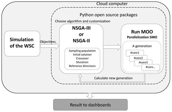
Figure 1.
Conceptual model of the SMO framework.
2.3. Delivery Performance Objectives
The main outputs of the DES are the function values for the four objectives: LT, BL, loss BL, and . LT is calculated as the total mean time from harvesting to customer delivery for all products. BL represents the mean accumulated delivery delays in cubic meters for all products, which cannot decrease, unlike backorders which measure delayed deliveries over a specific period (months). To improve the robustness of DeP, i.e., to minimize variations, a quadratic loss function [27] is included with the target function (expected to be close to zero), for the expected scaled loss in BL, , for a harvest schedule x [28]. The loss function includes both variance and standard deviation in the BL for product p to minimize delivery variation and improve robustness, e.g., by minimizing the product-weighted total mean (squared) and variance in the BL. The product-weighted objective CoV for BL is included to suppress variations between BLs, i.e., the standard deviation within total annual BLs, which is not reflected in the loss function; either factor can contribute to a high loss. The mathematical formulation of these objectives is given as Equations (1)–(5) below:
where represents the number of replications in the simulations per harvest solution and represents the variance for the same iterations. No covariance between products is considered; the variances are independent for each product p, where the weights reflect the relative contribution of each product to the total variance. When calculating and , it is assumed that demand and therefore BL are correlated with the production of each product, and in this study, no covariance between products is considered.
| P | products, |
| T | time, |
| weight of demand for product p | |
| standard deviation for BL for product p | |
| loss function for BL |
2.4. Discrete Event Simulation of Objectives
The DES [13] is based on real data from forest companies, as well as data used by most forest companies in Sweden, provided by the Biometria forest data hub, which collects most forest data in Sweden, and the Swedish Meteorological and Hydrological Institute (SMHI) for weather data that affect landing accessibility. Stand data include information on which stands are available to cut each year, their geographic positions, estimated product volumes, and stand type, thinning, or final felling. The harvesting team capacity depends on the type of felling, the density of the stem, and the distance from the site. The harvested wood is forwarded to the landings, where it is continually picked up by trucks, loading 40 m3, to be transported to customers if the road is accessible. Road accessibility is constrained by road class and weather during that week, which determines whether the landing is accessible [2,5]. The distances between each landing and the customer, traveled by truck transport, were given from the truck routing tool Krönt Vägval [34] and the Swedish National Road Database (SNVDB). Further details of the DES model are described in Westlund et al. [13].
The DES model is called from the MOO Python script to evaluate the four objective functions for an input harvest schedule, returning the objectives to the MOO algorithm. The harvest schedule specifies the annual sequence of harvest sites to harvest. This schedule is prepared to meet the customer demand for specific product groups and delivery time limits. The harvesting team operates according to this schedule, where parallel teams work simultaneously at different sites selected from the sequence. The objectives are recorded for each product and time period for each monthly demand. The modeled products are spruce sawlogs (SS), pine sawlogs (PS), spruce pulp (SP), conifer pulp (CP), and deciduous pulp (DP), i.e, five products where demand differs: the demand for SS is 29%, while that for PS is 27%, SP is 22%, CP is 15% and DP is 7%.
2.5. Genetic Algorithms for Harvest Scheduling
NSGA-II is a well-known MOO algorithm effective for handling two to four objectives using the non-dominated sorting mechanism [8,9]. The use of an elitist selection procedure, crowding distance, as a measure for comparison and selection after non-dominated sorting helps preserve the diversity of the population’s solutions. It is effective for finding the Pareto fronts of numerous practical problems [7]. NSGA-III [11] was proposed in 2014 to address many (>3 specifically) objective optimization problems. Like its predecessor NSGA-II, NSGA-III consistently emphasizes non-dominated solutions. However, unlike NSGA-II, NSGA-III replaces the crowding-distance-based diversity-preservation operator with a reference-direction-based strategy to maintain spread and diversity between its solutions on the Pareto front [11]. Throughout the optimization process, each feasible solution is aligned with a reference direction from a set of predefined directions. These reference directions can be set uniformly in the absence of any preference information among objectives or preferably adjusted to represent the preferences of the decision-maker [35]. The most commonly used method to define reference points is Das and Dennis’ structured method [36], which indicates direction vectors that originate from the origin. Each reference direction is divided into steps, or partitions, along the objective axis that guide the search for solutions. This allows NSGA-III to demonstrate improved performance compared to NSGA-II by effectively balancing exploration and exploitation, thereby ensuring a more representative set of optimal solutions in many-objective scenarios.
2.6. Genetic Algorithm Operators
Both NSGA-II [8] and NSGA-III [11] require customization of the genetic operators, including mutation and crossover, for optimization. The harvest scheduling problem is a permutation problem with similarities to the Traveling Salesman Problem. The NSGA-II algorithm has been used for a long time in MOO and to solve combinatorial problems such as the Traveling Salesman Problem. In Westlund et al. [13], the authors explored various genetic operators for a similar harvest scheduling permutation problem, concluding that the Partially Mapped Crossover developed by Goldberg and Lingle [37] performs well for this type of problem in combination with the inverse mutation operator, which was applied in this study.
Both GAs follow the same overall procedure, starting with an initial population, evaluating the current solutions, and improving the population in the next generation. The solutions in a GA are ranked relative to one another. A solution dominates another solution in the population if performs as well as in all objectives and is strictly better than in at least one objective. The non-dominated solutions form the first rank, i.e., the Pareto front. The difference between the methods lies in the reference directions that NSGA-III requires to guide the algorithm in searching for a good spread of the front. The reference direction is calculated from where H is the number of reference points, M is the number of objectives, and p is the division of each objective axis. Hence, the population size should be at least as large as the reference points, which causes the population for NSGA-III to grow when the reference directions increase.
3. Experiments, Results and Analysis
3.1. Computational Implementation
The required number of simulation evaluations to run a single SMO experiment is determined by the population size times the generation size. This means that for a population of 100 (harvest schedule sequences) and 100 generations, 10,000 simulations are to be executed. Despite this large number of simulation evaluations, a single generation can be evaluated in parallel using multiple CPUs, allowing the total time required for an SMO experiment to be significantly reduced.
In these experiments, an Azure Virtual Machine On-Demand with 16 CPUs was used. NSGA-III was run for a population of 100 solutions and 100 generations using 12 cores for about 22 h. The Python package dask [38] was used to parallelize the NSGA-II/III [8,11]. Dask [38] is a flexible, open-source Python parallel computing library that enables the execution of computations by scheduling tasks across multiple cores or distributed systems, and it provides progress monitoring in a web GUI. The integrated MOO drives the parallel simulation in the dashed part of Figure 1; a detailed explanation of the parallel process is described in Algorithm 1.
| Algorithm 1 SMO Parallel Processing Algorithm |
|
3.2. Comparative Experiments
Each SMO experiment was run for 100 generations with a population of 100 solutions per generation and five replications for each harvest scheduling simulation. NSGA-III was defined with a population of more than 84, using reference directions in six partitions and the Das-Dennis method to create them. The choice of partitions determines how many points are sampled for the search directions, which should match or exceed the population size. Since the experiments for NSGA-II and NSGA-III should have as similar prerequisites as possible, the maximum partition was set close to a population of 100.
The same setup was run for both NSGA-III and NSGA-II to compare the generated Pareto front solutions. The Pareto solutions are shown in the pairwise objectives plot in Figure 2: in purple for NSGA-III and green for NSGA-II. The loss BL is scaled with the natural logarithm for readability. NSGA-III found 26 solutions, while NSGA-II found 100. The differences between the solutions can be seen in the pattern: for example, in the top row of the first two plots in Figure 2, where NSGA-II provides many suggestions, but density varies along the front. As mentioned, NSGA-II uses crowding distance to promote the spread of solutions, while NSGA-III uses a reference-direction-based niching strategy to maintain diversity, as shown in the solution spread in Figure 2. NSGA-III provides fewer solutions, but they are evenly distributed across the front. The spread of solutions results in better overall performance with lower objective values. For mean BL versus loss BL, the solutions revealed a strong tendency to converge. In the fourth column, the CoVBL value is shown. This objective does not show a clear front, but overall, NSGA-III finds lower values for the objective than the more scattered solutions. In NSGA-II, most solutions have higher values of objective functions three () and four () than those of NSGA-III. NSGA-III demonstrates better performance than NSGA-II despite having fewer solutions on the Pareto front.
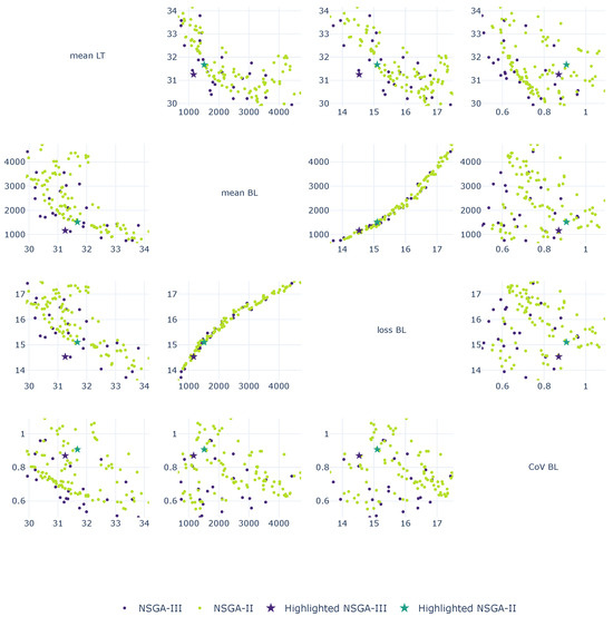
Figure 2.
NSGA-III (purple) and NSGA-II (green) solutions for pairwise objectives. Marked solutions are for a follow-up in a dashboard visualization.
To evaluate the quality of the solutions, hypervolume can be used as a performance indicator [39,40]. It describes how much of the space, or coverage in space, is dominated by the solutions in relation to a reference point. The covered space is the volume between the solution and the reference point. Larger hypervolume values indicate a better spread of solutions and performance when comparing algorithms. The hypervolume for both GAs is shown in Figure 3, indicating that the performance of NSGA-III is better than that of NSGA-II already in the first generations. NSGA-II does not approach NSGA-III until around generation 60 but it performs worse.
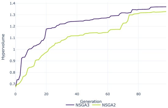
Figure 3.
Hypervolume comparison of NSGA-III and NSGA-II.
In Figure 4, the convergence of the objective is shown for both GAs and all objectives. It can be seen that for all objectives, NSGA-III converges faster during the first approximately 20 generations. It also shows a different pattern of convergence later, showing more fluctuations during convergence. After about 90 generations, the pattern stabilizes for both GAs.
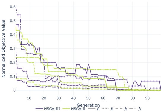
Figure 4.
Convergence of objectives NSGA-II (green) and NSGA-III (purple).
Figure 5 shows a boxplot for the four objectives and GAs for the normalized objectives. For all objectives, the solutions after 100 generations show, on average, lower mean and median values in NSGA-III compared to NSGA-II—a shorter LT in days from harvesting to customer delivery, fewer backlogs in deliveries, and less variation in deliveries given from the BL loss. For CoV, NSGA-II and III show similar results, indicating that the variance in backlogs relative to the mean is quite similar. However, in NSGA-III, the CoV shows a slightly wider spacing between quartiles, indicating a greater spread around the median and, overall, a slightly greater variability in the solutions of this method. A larger interquartile range indicates that half of the solutions are more spread out, reflecting greater dispersion and more extreme variations.
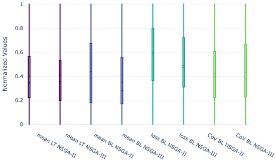
Figure 5.
Boxplot comparison of NSGA-II and NSGA-III.
3.3. Simulation and Visualization for Decision Making
The forest manager, as a decision-maker, is likely interested in the practical application of the framework and how a solution affects individual product deliveries. DES is a supporting tool that enables the simulation and evaluation of solutions, providing deeper insight into the WSC when a solution is applied. The DES is adaptable and can log more data to study the WSC. Figure 2 shows the available solutions of harvest schedules of 100 generations to select from. For a decision-maker, the details in the solution are of interest. For example, it can be of interest to analyze the impact of a solution: for example, how deliveries of individual products perform over time.
Figure 2 shows two solutions picked (marked as stars) with a trade-off on the mean LT and the mean BL from the front for NSGA-III and NSGA-II. The two solutions are simulated in the DES where the details of specific products are logged. Figure 6 shows the simulated NSGA-III solution, and Figure 7 shows the NSGA-II solution. On the right y-axis is the BL shown, and on the left y-axis is the backorder, i.e., the difference in BLs for all months (non-delivered m3s). For all products, the BL is higher in the NSGA-II solution at the end of the year. Sawlogs have higher total BL and backorders are higher overall in NSGA-II, where the occurrence of BL varies in months for the two solutions. Deciduous pulp varies over the months for both solutions, with a large BL, even though it is lower in NSGA-III. Deciduous pulp is difficult to calculate harvest outcomes for, as it is a small product harvested when available at a site. Small volumes are collected at scattered harvesting sites to meet demand. Regardless of the GA algorithm, the range of variations will be large because availability occurs in spurts across different harvesting areas despite an annual scheduling. In both Figure 6 and Figure 7, an increase in BL and backorder is observed in spring and the beginning of summer, April–June. The thawing period starts in April and affects landing accessibility, impacting deliveries until the beginning of summer, and decreasing DeP during this time. However, a difference in backlogs is observed for these months with both NSGA-III backlogs and backorders falling below NSGA-II for all products.
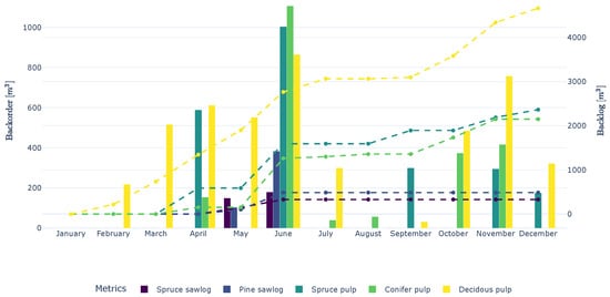
Figure 6.
Simulated NSGA-III marked in Figure 2. Backorders are shown as bars, and backlogs as dashed lines.
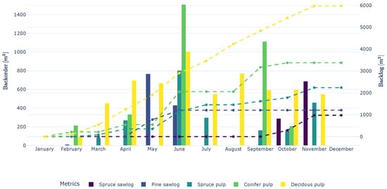
Figure 7.
Simulated NSGA-II solution marked in Figure 2. Backorders are shown as bars, and backlogs as dashed lines.
Table 1 shows the values of the objective functions from the simulation of the two solutions. As already shown in Figure 2, NSGA-III should give better performance in mean LT and BL than NSGA-II, as shown in both Figure 2 and when the solution is simulated in DES in Figure 7.

Table 1.
Objective functions values.
4. Discussion
4.1. Optimization Objectives
The choice of objectives depends on the decision-maker’s preference. Lead time and delivery on time, suppressing variations, are important in the WSC but are also general objectives for many supply chains [14]. Two different objective functions are used for exploratory analysis that addresses variations, which are amplified by uncertain road accessibility [3,4]. Backlogs can be more accepted as long as they are smooth, e.g., it is better to know that the same backlog occurs over the year. One objective addresses product-weighted backlog variations, and the other focuses on the standard deviation relative to the mean backlog. In this study, no covariance between the products is considered. This is based on the fact that a tree of one species is bucked into that category of products, which is expected not to affect other products from other bucked tree species. For example, a spruce bucked into sawlogs does not affect deciduous pulp logs of a deciduous tree. However, other assumptions could be made to determine whether there are relationships between the products produced. In this experiment, the CoV objective is used to minimize delivery variance, as this aspect is not explicitly addressed in the loss function. Even if backlogs are generally low or close to zero, high delivery variance can still negatively impact the total loss function, potentially increasing it. In this study, the weights represent the share of the total product volume. This weight factor could be chosen differently depending on preferences. The product-weighted annual backlog-loss function indicates convergence with the total backlog across all products. This could have simplified the search for solutions. However, since NSGA-III is more effective for problems with more than three objectives, the solutions indicate that despite this, NSGA-III could perform better than NSGA-II and therefore has not negatively affected the results. The weights could be based on importance, value, or other factors that could change the behavior of the function and hence its convergence. This suggests changing the loss function, where using backorders (based on the mean and standard deviation for each specific month) could be a better choice to minimize the risk of redundancy [28]. Hence, the objectives related to variation may evolve, and additional objectives could be introduced to address specific types of variation, thereby improving the robustness of deliveries within the model. In future studies, other types of variation could be interesting to include and possibly mitigate their impact on DeP, such as variations in harvested product volumes or demand. The DES functions both as a tool for computing complex objective functions and for the post-optimality analysis of specific solutions, enhancing understanding of their impact. The DES provides the NSGA-III with WSC data, but it is also shown how simulating can be used to re-run a harvest schedule solution for more details. They serve as a basis for visualizing more detailed results for a decision-maker and as a suggestion for dashboard information (Figure 6 and Figure 7). More information could be collected from the DES, including details of processes, etc., to support on-demand analyses for decision-makers. The potential of the DES-based approach for decision support can be further explored by simulation to provide more information on what a solution entails, including additional outputs such as logged values for product inventory levels and the progress over time of the DeP objectives.
4.2. Computational Issues
In this study, the SMO framework was parallelized and run on a cloud platform using multiple on-demand CPU cores to speed up calculations. For a research project, 16 cores are sufficient to produce results in a reasonable time. More CPU resources will further reduce computational time because each core contributes to solving a single solution in the population. For larger populations (e.g., above 100), the equivalent number of CPUs makes the framework run faster in a production environment. For future work, the possibility of running GAs on a GPU [41] may also be of interest, which should be able to speed up the calculations further and bring the framework one step closer to a production environment.
4.3. Managerial Implications
Planning and scheduling in real-world applications often involve multiple targets. This is highlighted by Acuna et al. [6], calling for more multi-objective decision support for forest biomass supply chains. Ulvdal et al. [1] shows that, despite the existing support tools, much of the tactical and operational planning, to which harvest scheduling belongs, is manual. This study, aimed at improving methods for harvest scheduling decision support, addresses this challenge by exploring how objectives associated with different entities can be simultaneously managed within the scheduling process. The goal is to generate more optimal schedules that meet many delivery goals. It can guide forest managers first to calculate harvest schedules that reflect many objective preferences and then evaluate which schedules best meet the defined DeP goals while highlighting the trade-offs involved. NSGA-II is widely applied to a broad range of scheduling problems for various purposes [9]. However, as Rahimi et al. [9] note, fewer than 1% of NSGA-II–based scheduling studies address many-objective problems. To incorporate additional objectives for more robust scheduling, the genetic algorithm must also be capable of handling the increased dimensionality. Searching the Pareto front effectively requires different methods for evolutionary multi-objective and many-objective problems, as algorithm performance varies depending on the problem characteristics [42]. For multi-objective problems, NSGA-II relies on crowding distance, which is effective for up to three objectives. In contrast, NSGA-III uses reference directions, which provide better coverage of the Pareto front when dealing with four or more objectives [11]. NSGA-III therefore becomes more robust than NSGA-II as the number of objectives increases. The results of this study show that NSGA-III can serve as an alternative to NSGA-II for harvest scheduling problems with more than three objectives, to identify well-distributed Pareto front solutions. Given the computational demands of evolutionary algorithms, particularly NSGA-III [11], parallel evaluations using on-demand computational resources are advantageous. This improves scalability and shortens the path to deploying the method as an industrial decision-support tool for harvest scheduling with multiple delivery objectives.
This study focuses on harvest scheduling, which is a permutation-based planning problem. Although calculating supply-chain objectives using analytical functions can be complex, it is feasible through simulation. In other supply-chain studies, it is believed that a suitable simulation model could be used similarly to evaluate sequencing or planning decisions to achieve high-performance goals. Conceptually, the combination of NSGA-III (or NSGA-II) with a simulation-based evaluation of complex supply-chain objectives for MOO can be applied to a wide range of permutation-based scheduling and planning problems commonly found in supply-chain contexts.
5. Conclusions
In this paper, NSGA-III [11] has been adopted in the SMO framework [13,28]. A comparison of NSGA-III for a multi-objective problem with the well-known NSGA-II algorithm for harvest scheduling across four DeP objectives has been evaluated. The WSC was simulated in a DES using information on product demand, road accessibility, and harvesting and transport data derived from real-world data. Improvements in faster solution generation were achieved by parallelizing SMO calculations using the Microsoft Azure cloud service, reducing the time required for a single SMO experiment from a week to one day.
It has been shown that NSGA-III is an alternative to NSGA-II for finding harvest schedules with many objectives, providing both a better spread of the Pareto front as verified by the hypervolume metric and more optimal DeP objective values. NSGA-III could be an alternative to replace NSGA-II in the SMO framework for harvest scheduling [13] for more than three delivery objectives.
Author Contributions
Conceptualization, K.W. and A.H.C.N.; methodology, K.W. and A.H.C.N.; software, K.W. and A.H.C.N.; validation, K.W. and A.H.C.N.; formal analysis, K.W.; writing—original draft preparation, K.W. and A.H.C.N.; writing—review and editing, A.H.C.N.; visualization, K.W.; supervision, A.H.C.N. All authors have read and agreed to the published version of the manuscript.
Funding
This research was supported by the Swedish Foundation for Strategic Research through the project FID17-0043.
Data Availability Statement
Restrictions apply to the availability of these data. The data used in this study were obtained from a previous research project described in [5]; therefore, no real company data are disclosed.
Conflicts of Interest
No company was involved in the study design, data analysis, interpretation of the results, or manuscript preparation. The authors declare no conflicts of interest.
Abbreviations
The following abbreviations are used in this manuscript:
| BL | Backlog |
| CoV | Coefficient of Variation |
| CP | Conifer pulpwood |
| DES | Discrete Event Simulation |
| DeP | Delivery performance |
| GA | Genetic algorithm |
| LT | Lead time |
| MOO | Multi-objective optimization |
| PS | Pine sawlogs |
| SMO | Simulation-based Multi-Objective Optimization |
| SS | Spruce sawlogs |
| SP | Spruce pulpwood |
| WSC | Wood supply chain |
References
- Ulvdal, P.; Öhman, K.; Eriksson, L.O.; Wästerlund, D.S.; Lämås, T. Handling Uncertainties in Forest Information: The Hierarchical Forest Planning Process and Its Use of Information at Large Forest Companies. For. Int. J. For. Res. 2023, 96, 62–75. [Google Scholar] [CrossRef]
- Biometria. Klassning av Skogsbilvägar [Classification of Forest Roads]. Available online: https://www.biometria.se/media/fa1ba4qc/klassning-av-skogsbilvaegar_september-2021_webb.pdf (accessed on 27 April 2023).
- Lehtonen, I.; Venäläinen, A.; Kämäräinen, M.; Asikainen, A.; Laitila, J.; Anttila, P.; Peltola, H. Projected decrease in wintertime bearing capacity on different forest and soil types in Finland under a warming climate. Hydrol. Earth Syst. Sci. 2019, 23, 1611–1631. [Google Scholar] [CrossRef]
- Kellomäki, S.; Maajärvi, M.; Strandman, H.; Kilpeläinen, A.; Peltola, H. Model Computations on the Climate Change Effects on Snow Cover, Soil Moisture and Soil Frost in the Boreal Conditions over Finland. Silva Fenn. 2010, 44, 213–233. [Google Scholar] [CrossRef]
- Westlund, K.; Sundström, L.E.; Eliasson, L. An optimization and discrete event simulation framework for evaluating delivery performance in Swedish wood supply chains under stochastic weather variations. Int. J. For. Eng. 2024, 35, 326–337. [Google Scholar] [CrossRef]
- Acuna, M.; Sessions, J.; Zamora, R.; Boston, K.; Brown, M.; Ghaffariyan, M.R. Methods to Manage and Optimize Forest Biomass Supply Chains: A Review. Curr. For. Rep. 2019, 5, 124–141. [Google Scholar] [CrossRef]
- Sharma, S.; Kumar, V. A Comprehensive Review on Multi-objective Optimization Techniques: Past, Present and Future. Arch. Comput. Methods Eng. 2022, 29, 5605–5633. [Google Scholar] [CrossRef]
- Deb, K.; Pratap, A.; Agarwal, S.; Meyarivan, T. A fast and elitist multiobjective genetic algorithm: NSGA-II. IEEE Trans. Evol. Comput. 2002, 6, 182–197. [Google Scholar] [CrossRef]
- Rahimi, I.; Gandomi, A.H.; Deb, K.; Chen, F.; Nikoo, M.R. Scheduling by NSGA-II: Review and Bibliometric Analysis. Processes 2022, 10, 98. [Google Scholar] [CrossRef]
- Verma, S.; Pant, M.; Snasel, V. A Comprehensive Review on NSGA-II for Multi-Objective Combinatorial Optimization Problems. IEEE Access 2021, 9, 57757–57791. [Google Scholar] [CrossRef]
- Deb, K.; Jain, H. An Evolutionary Many-Objective Optimization Algorithm Using Reference-Point-Based Nondominated Sorting Approach, Part I: Solving Problems with Box Constraints. IEEE Trans. Evol. Comput. 2014, 18, 577–601. [Google Scholar] [CrossRef]
- Talbi, E.G.; Mostaghim, S.; Okabe, T.; Ishibuchi, H.; Rudolph, G.; Coello Coello, C.A. Parallel Approaches for Multiobjective Optimization. In Multiobjective Optimization: Interactive and Evolutionary Approaches; Branke, J., Deb, K., Miettinen, K., Słowiński, R., Eds.; Lecture Notes in Computer Science; Springer: Berlin/Heidelberg, Germany, 2008; Volume 5252, pp. 349–372. [Google Scholar] [CrossRef]
- Westlund, K.; Ng, A.H.; Nourmohammadi, A. Simulation-Based Multi-Objective Optimization to Support Delivery Performance Decisions in Harvest Scheduling and Transport. Int. J. For. Eng. 2025, 0, 1–14. [Google Scholar] [CrossRef]
- Gunasekaran, A.; Patel, C.; McGaughey, R.E. A framework for supply chain performance measurement. Int. J. Prod. Econ. 2004, 87, 333–347. [Google Scholar] [CrossRef]
- Karlsson, J.; Rönnqvist, M.; Bergström, J. An Optimization Model for Annual Harvest Planning. Can. J. For. Res. 2004, 34, 1747–1754. [Google Scholar] [CrossRef]
- Ene, L.T.; Söderberg, J.; Möller, J. Volume and Value Recovery Predictions by Combining Tree Lists from a Harvester Stem Database and Estimated Diameter Distributions from a Mobile Laser Scanner System. Available online: https://www.skogforsk.se/cd_20211215112543/contentassets/52b3596dfe804c1b94621905487b9315/arbetsrapport-1103-2021.pdf (accessed on 1 December 2023).
- Kogler, C.; Rauch, P. Lead time and quality driven transport strategies for the wood supply chain. Res. Transp. Bus. Manag. 2023, 47, 100946. [Google Scholar] [CrossRef]
- Palander, T.; Tokola, T.; Borz, S.A.; Rauch, P. Forest Supply Chains During Digitalization: Current Implementations and Prospects in Near Future. Curr. For. Rep. 2024, 10, 223–238. [Google Scholar] [CrossRef]
- Stewart, G. Supply chain performance benchmarking study reveals keys to supplychain excellence. Logist. Inf. Manag. 1995, 8, 38–44. [Google Scholar] [CrossRef]
- Gunasekaran, A.; Patel, C.; Tirtiroglu, E. Performance measures and metrics in a supply chain environment. Int. J. Oper. Prod. Manag. 2001, 21, 71–87. [Google Scholar] [CrossRef]
- Kogler, C.; Rauch, P. Discrete event simulation of multimodal and unimodal transportation in the wood supply chain: A literature review. Silva Fenn. 2018, 52, 9984. [Google Scholar] [CrossRef]
- Chen, C.; Gan, J.; Zhang, Z.; Qiu, R. Multi-Objective and Multi-Period Optimization of a Regional Timber Supply Network with Uncertainty. Can. J. For. Res. 2020, 50, 203–214. [Google Scholar] [CrossRef]
- Shavazipour, B.; Kwakkel, J.H.; Miettinen, K. Let Decision-Makers Direct the Search for Robust Solutions: An Interactive Framework for Multiobjective Robust Optimization under Deep Uncertainty. Environ. Model. Softw. 2025, 183, 106233. [Google Scholar] [CrossRef]
- Simard, V.; Rönnqvist, M.; LeBel, L.; Lehoux, N. Improving the Decision-Making Process by Considering Supply Uncertainty—A Case Study in the Forest Value Chain. Int. J. Prod. Res. 2024, 62, 665–684. [Google Scholar] [CrossRef]
- Hopp, W.J. Supply Chain Science, 1st ed.; Waveland Press: Long Grove, IL, USA, 2011. [Google Scholar]
- Pound, E.; Bell, J.; Spearman, M. Factory Physics for Managers: How Leaders Improve Performance in a Post-Lean Six SIGMA World, 1st ed.; McGraw Hill: New York, NY, USA, 2014. [Google Scholar]
- Sanchez, S.M.; Sanchez, P.J. Robustness Revisited: Simulation Optimization Viewed Through A Different Lens. In Proceedings of the 2020 Winter Simulation Conference (WSC), Orlando, FL, USA, 14–18 December 2020; IEEE: Piscataway, NJ, USA, 2020; pp. 60–74. [Google Scholar] [CrossRef]
- Westlund, K.; Ng, A.H. Analyzing Delivery Performance and Robustness of Wood Supply Chains Using Simulation-Based Multi-Objective Optimization. In Proceedings of the 2024 Winter Simulation Conference (WSC), Orlando, FL, USA, 15–18 December 2024; IEEE: Piscataway, NJ, USA, 2024; pp. 1587–1598. [Google Scholar] [CrossRef]
- Deb, K.; Mohan, M.; Mishra, S. Towards a Quick Computation of Well-Spread Pareto-Optimal Solutions. In Evolutionary Multi-Criterion Optimization; Springer: Berlin/Heidelberg, Germany, 2003; Volume 2632, pp. 222–236. [Google Scholar] [CrossRef]
- Neumann, A.; Hajji, A.; Rekik, M.; Pellerin, R. Genetic algorithms for planning and scheduling engineer-to-order production: A systematic review. Int. J. Prod. Res. 2024, 62, 2888–2917. [Google Scholar] [CrossRef]
- Pătrăușanu, A.; Florea, A.; Neghină, M.; Dicoiu, A.; Chiș, R. A Systematic Review of Multi-Objective Evolutionary Algorithms Optimization Frameworks. Processes 2024, 12, 869. [Google Scholar] [CrossRef]
- Blank, J.; Deb, K. Pymoo: Multi-Objective Optimization in Python. IEEE Access 2020, 8, 89497–89509. [Google Scholar] [CrossRef]
- Ng, A.H.C.; Bernedixen, J. Production systems analysis and optimization using facts analyzer. In Proceedings of the 2018 Winter Simulation Conference, Gothenburg, Sweden, 9–12 December 2018; IEEE Press: Piscataway, NJ, USA, 2018; p. 4258. [Google Scholar]
- Svenson, G. Optimized Route Selection for Logging Trucks Improvements to Calibrated Route Finder. Ph.D. Thesis, Swedish University of Agricultural Sciences, Uppsala, Sweden, 2017. [Google Scholar]
- Li, B.; Li, J.; Tang, K.; Yao, X. Many-Objective Evolutionary Algorithms: A Survey. ACM Comput. Surv. 2015, 48, 13. [Google Scholar] [CrossRef]
- Das, I.; Dennis, J.E. Normal-Boundary Intersection: A New Method for Generating the Pareto Surface in Nonlinear Multicriteria Optimization Problems. SIAM J. Optim. 1998, 8, 631–657. [Google Scholar] [CrossRef]
- Goldberg, D.E.; Lingle, R. Alleles, Loci, and the Traveling Salesman Problem. In Proceedings of the First International Conference on Genetic Algorithms and Their Applications; Psychology Press: London, UK, 1985; pp. 154–159. [Google Scholar]
- Dask Development Team. Dask: Library for Dynamic Task Scheduling. Available online: http://dask.pydata.org (accessed on 1 March 2024).
- Auger, A.; Bader, J.; Brockhoff, D.; Zitzler, E. Hypervolume-based multiobjective optimization: Theoretical foundations and practical implications. Theor. Comput. Sci. 2012, 425, 75–103. [Google Scholar] [CrossRef]
- Guerreiro, A.P.; Fonseca, C.M.; Paquete, L. The Hypervolume Indicator: Computational Problems and Algorithms. ACM Comput. Surv. 2021, 54, 119. [Google Scholar] [CrossRef]
- He, J.; Liu, H.; Wu, Y.; Zheng, Z.; Zhu, T. A Preliminary Study on Accelerating Simulation Optimization with GPU Implementation. In Proceedings of the 2024 Winter Simulation Conference (WSC), Orlando, FL, USA, 15–18 December 2024; pp. 3458–3469. [Google Scholar] [CrossRef]
- Huband, S.; Hingston, P.; Barone, L.; While, L. A Review of Multiobjective Test Problems and a Scalable Test Problem Toolkit. IEEE Trans. Evol. Comput. 2006, 10, 477–506. [Google Scholar] [CrossRef]
Disclaimer/Publisher’s Note: The statements, opinions and data contained in all publications are solely those of the individual author(s) and contributor(s) and not of MDPI and/or the editor(s). MDPI and/or the editor(s) disclaim responsibility for any injury to people or property resulting from any ideas, methods, instructions or products referred to in the content. |
© 2026 by the authors. Licensee MDPI, Basel, Switzerland. This article is an open access article distributed under the terms and conditions of the Creative Commons Attribution (CC BY) license.