
Putting the Personalized Metabolic Avatar into Production: A Comparison between Deep-Learning and Statistical Models for Weight Prediction


 ,
,  ,
,  and
and 
Abstract
1. Introduction
2. Materials and Methods
2.1. Study Population
2.2. Wearables and Devices
- The MiBand 6, a smartband of Xiaomi Inc.® (Beijing, China), for estimating calories burned during exercise (walking, running, etc.).
- The Mi Body Composition Scale, an impedance balance of Xiaomi Inc.® (Beijing, China), for tracking weight and RMR.
2.3. Datasets
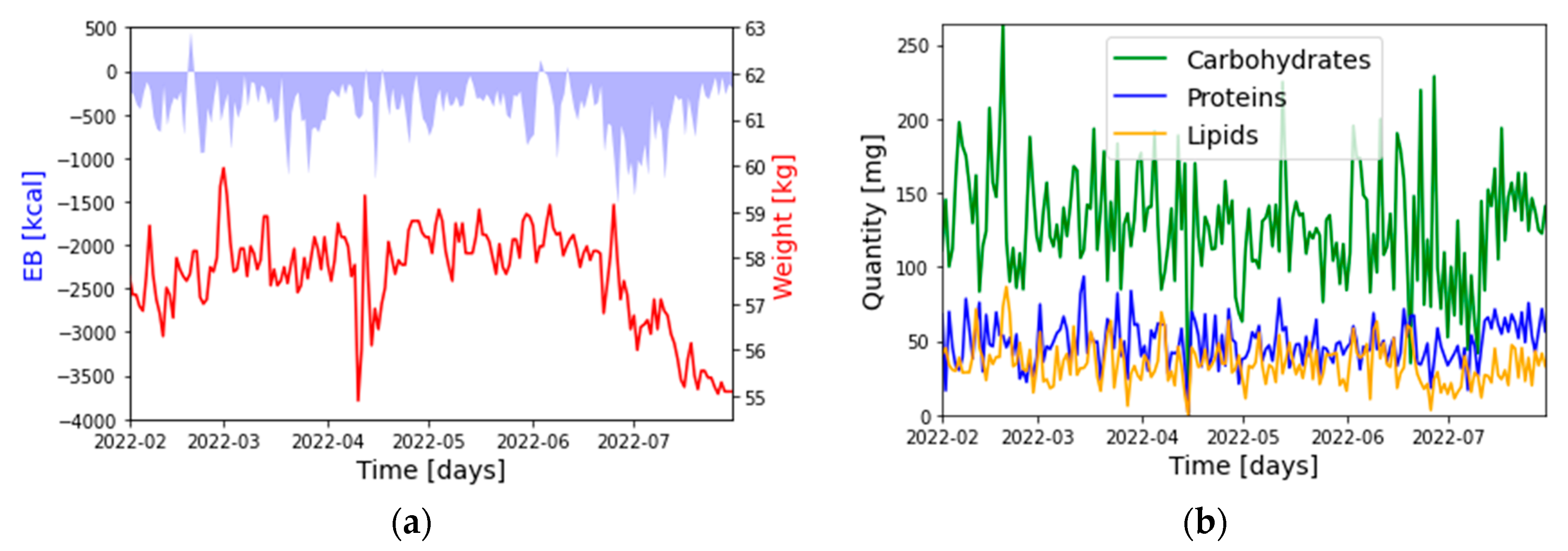
- : Weight: [kg]
- : Energy Balance (EB): [kcal]
- : Carbohydrates: [g]
- : Proteins: [g]
- : Lipids: [g]
2.4. Description of Models
- is the nonseasonal autoregressive lag polynomial;
- is the seasonal autoregressive lag polynomial;
- is the time series, differenced d times and seasonally differenced D times;
- is the nonseasonal moving average lag polynomial;
- is the seasonal moving average lag polynomial.
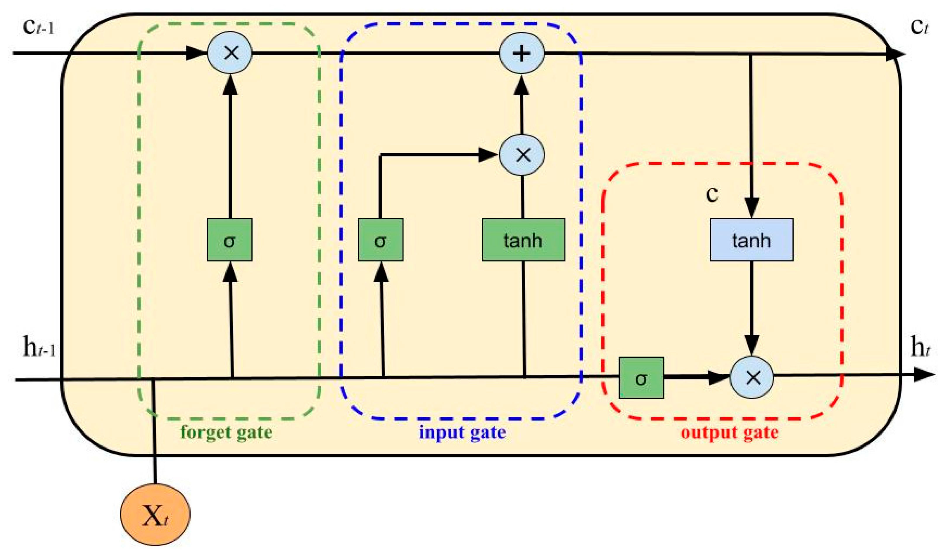
- Input Gate:
- Forget Gate:
- Output Gate:
- Intermediate Cell State:
- Cell State (Next Memory Input):
- New State:with as the input vector, as the output vector, W and U as parameter matrices and f as the parameter vector.
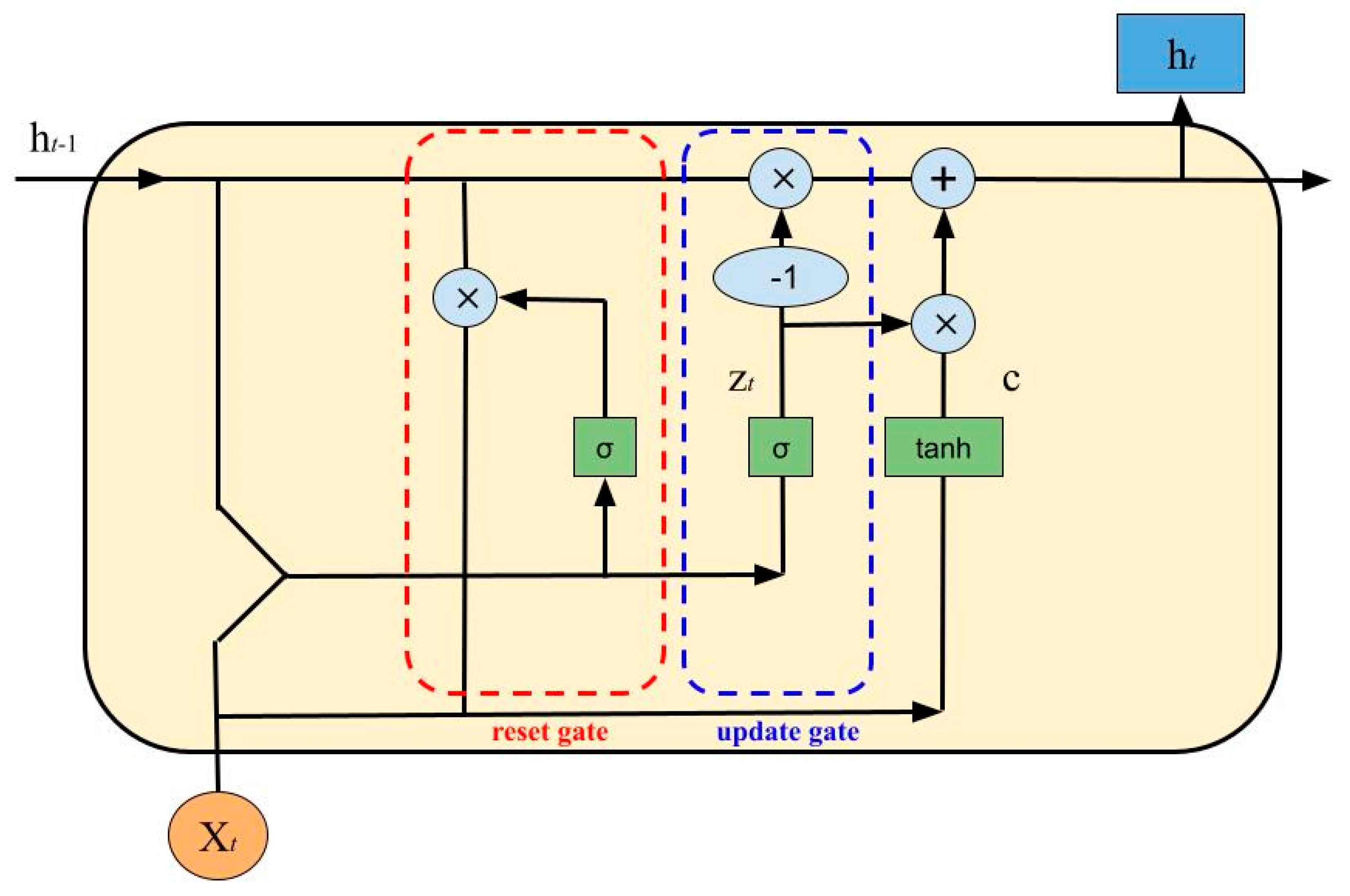
- Update Gate:
- Reset Gate:
- Cell State:
- New State:
2.5. Model Selection and Comparison
2.5.1. Implementation and Selection of Models
2.5.2. Performance of Models with Datasets of Varying Length
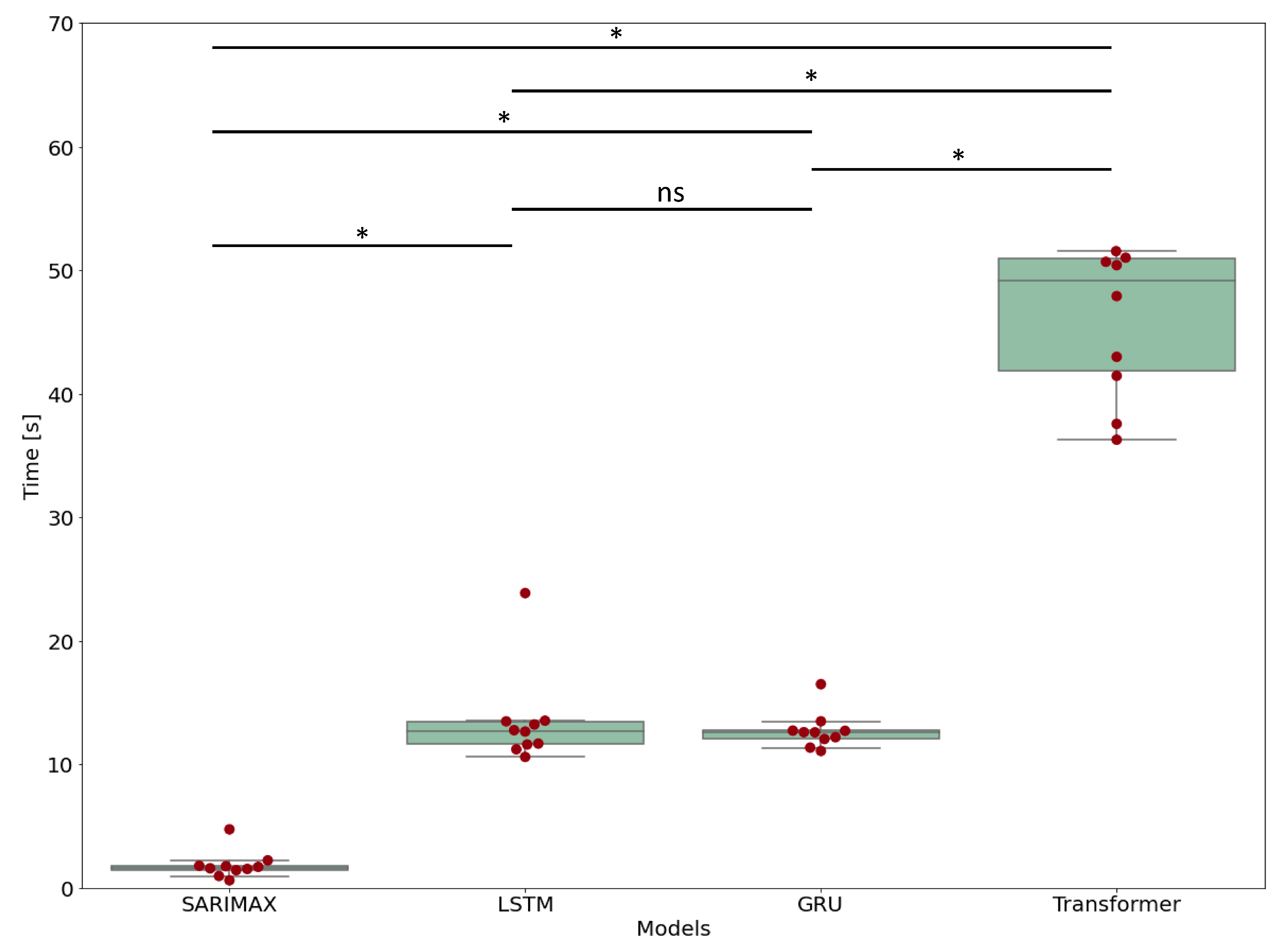
2.5.3. Computational Time
2.6. Computational Requirements and Python Libraries
3. Results
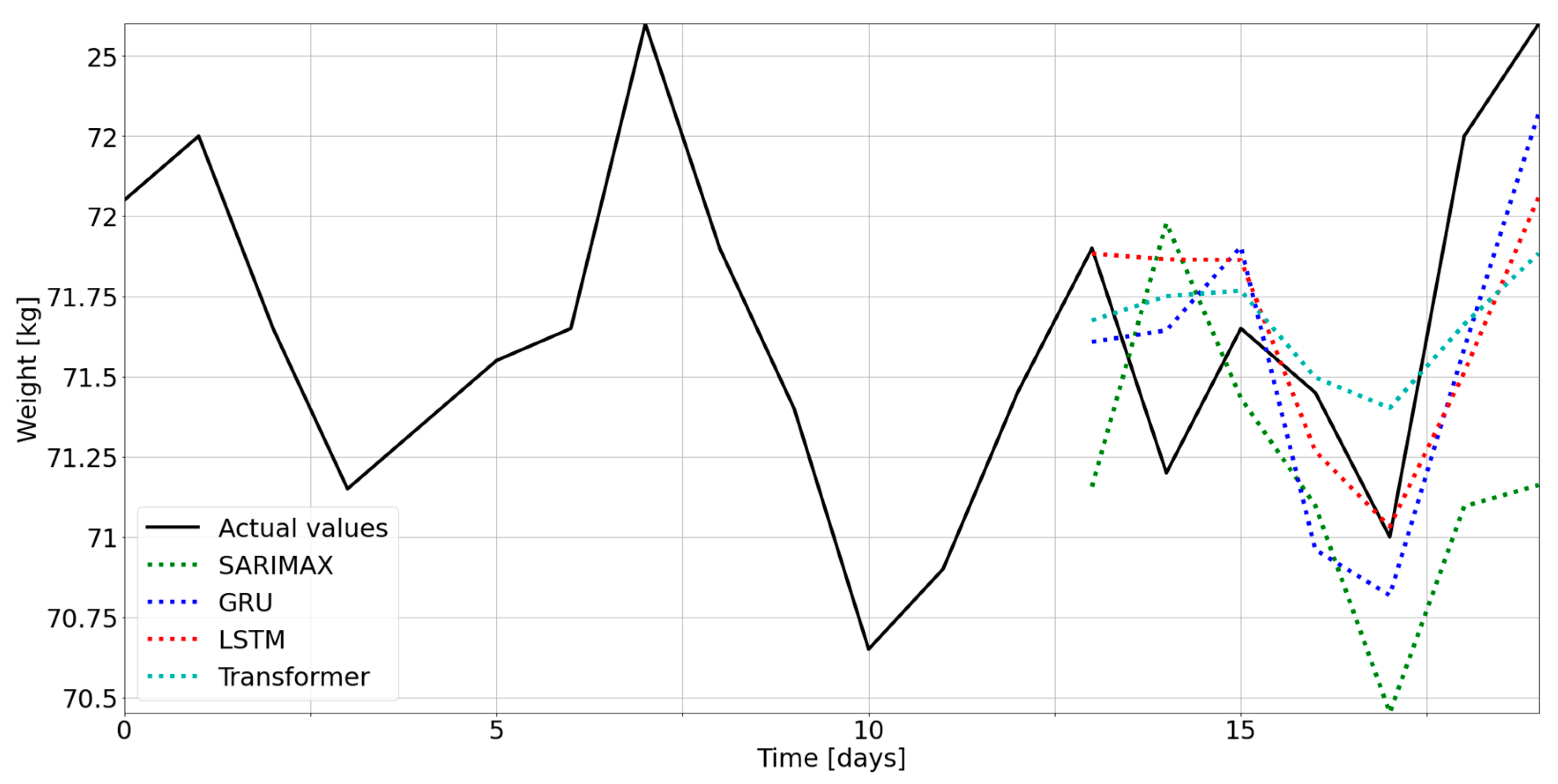
3.1. Selection of the Optimal Model
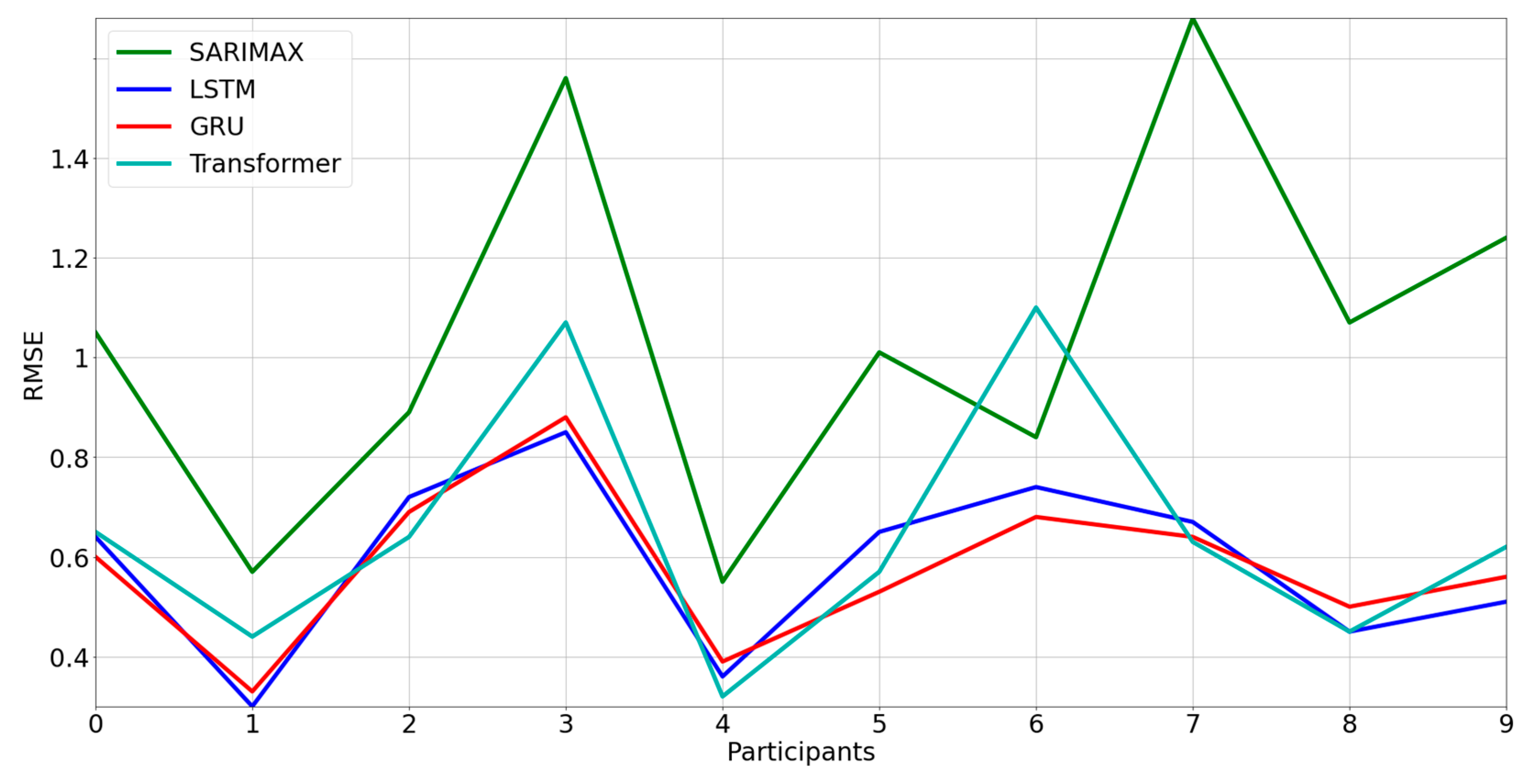
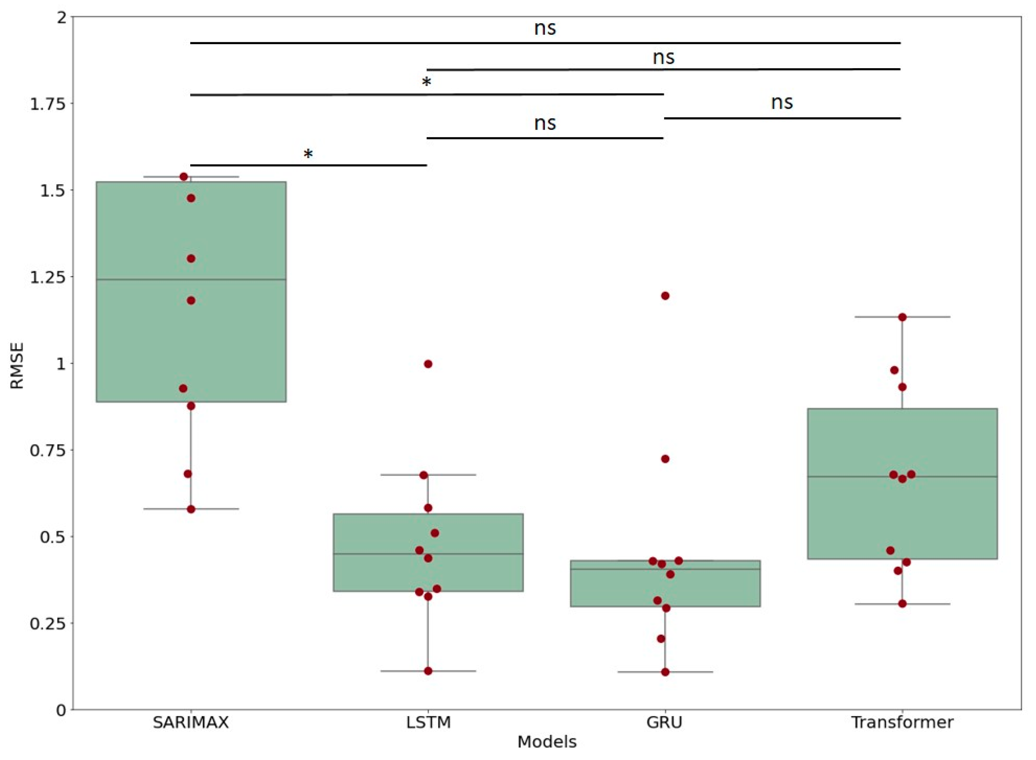
3.2. Comparison between Models
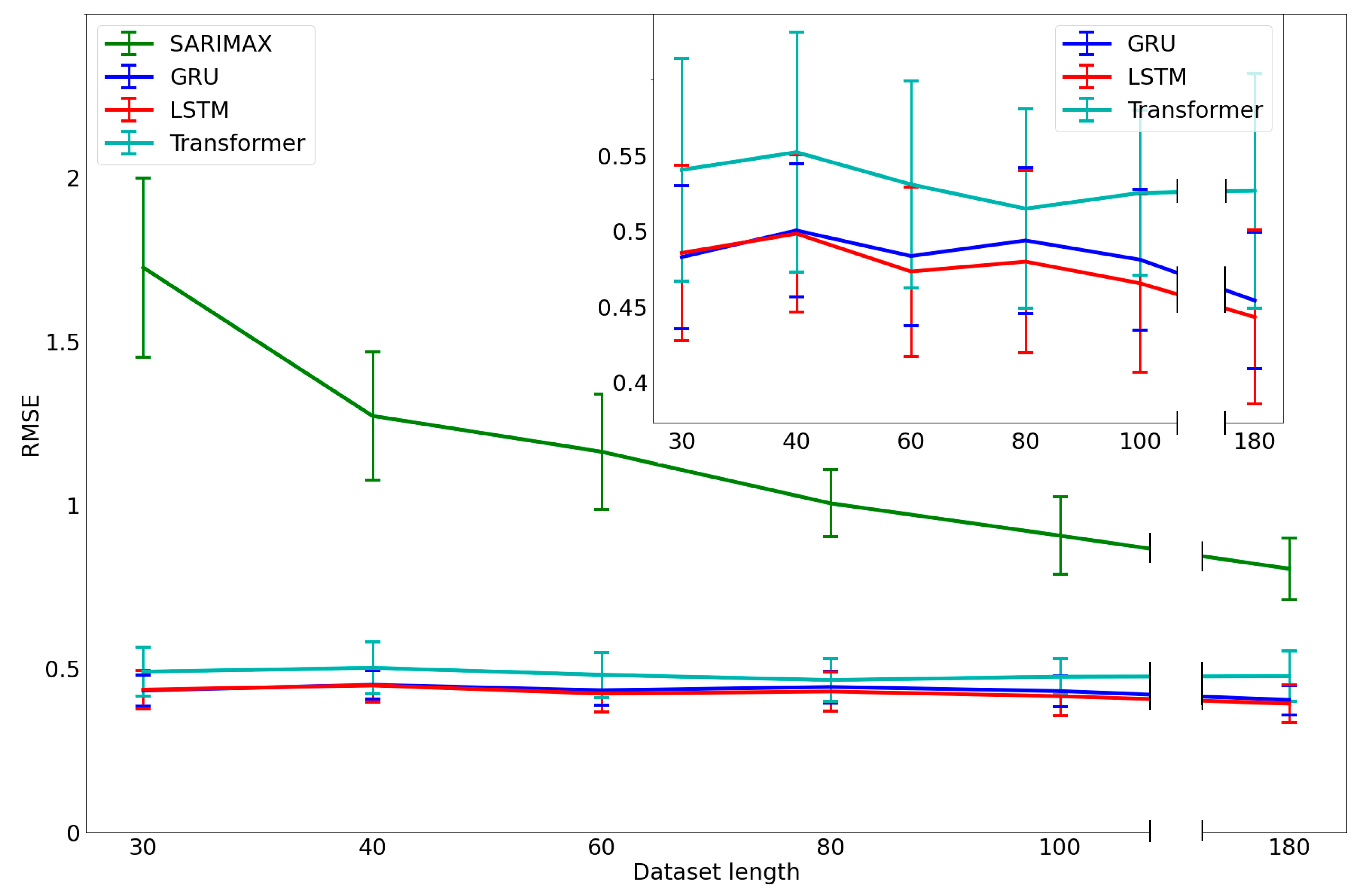
3.3. Analysis of the Performance with a Limited Dataset Length
3.4. Performance versus Data Length
3.5. Computational Time
4. Discussion
5. Conclusions
Supplementary Materials
Author Contributions
Funding
Institutional Review Board Statement
Informed Consent Statement
Data Availability Statement
Conflicts of Interest
References
- Mold, J. Goal-Directed Health Care: Redefining Health and Health Care in the Era of Value-Based Care. Cureus 2017, 9, e1043. [Google Scholar] [CrossRef]
- Bianchi, V.E. Impact of Nutrition on Cardiovascular Function. Curr. Probl. Cardiol. 2020, 45, 100391. [Google Scholar] [CrossRef]
- Wiseman, M.J. Nutrition and Cancer: Prevention and Survival. Br. J. Nutr. 2019, 122, 481–487. [Google Scholar] [CrossRef]
- Tourlouki, E.; Matalas, A.-L.; Panagiotakos, D.B. Dietary Habits and Cardiovascular Disease Risk in Middle-Aged and Elderly Populations: A Review of Evidence. Clin. Interv. Aging 2009, 4, 319–330. [Google Scholar] [CrossRef]
- Pignatti, C.; D’adamo, S.; Stefanelli, C.; Flamigni, F.; Cetrullo, S. Nutrients and Pathways That Regulate Health Span and Life Span. Geriatrics 2020, 5, 95. [Google Scholar] [CrossRef]
- Kussmann, M.; Raymond, F.; Affolter, M. OMICS-Driven Biomarker Discovery in Nutrition and Health. J. Biotechnol. 2006, 124, 758–787. [Google Scholar] [CrossRef] [PubMed]
- Chaudhary, N.; Kumar, V.; Sangwan, P.; Pant, N.C.; Saxena, A.; Joshi, S.; Yadav, A.N. Personalized Nutrition and -Omics. In Comprehensive Foodomics; Elsevier: Amsterdam, The Netherlands, 2020; pp. 495–507. ISBN 9780128163955. [Google Scholar]
- Iqbal, S.M.A.; Mahgoub, I.; Du, E.; Leavitt, M.A.; Asghar, W. Advances in Healthcare Wearable Devices. NPJ Flex. Electron. 2021, 5, 9. [Google Scholar] [CrossRef]
- Ahmadi-Assalemi, G.; Al-Khateeb, H.; Maple, C.; Epiphaniou, G.; Alhaboby, Z.A.; Alkaabi, S.; Alhaboby, D. Digital Twins for Precision Healthcare. In Advanced Sciences and Technologies for Security Applications; Springer: Berlin/Heidelberg, Germany, 2020; pp. 133–158. [Google Scholar]
- Mulder, S.T.; Omidvari, A.H.; Rueten-Budde, A.J.; Huang, P.H.; Kim, K.H.; Bais, B.; Rousian, M.; Hai, R.; Akgun, C.; van Lennep, J.R.; et al. Dynamic Digital Twin: Diagnosis, Treatment, Prediction, and Prevention of Disease During the Life Course. J. Med. Internet Res. 2022, 24, e35675. [Google Scholar] [CrossRef]
- Bianchetti, G.; Abeltino, A.; Serantoni, C.; Ardito, F.; Malta, D.; de Spirito, M.; Maulucci, G. Personalized Self-Monitoring of Energy Balance through Integration in a Web-Application of Dietary, Anthropometric, and Physical Activity Data. J. Pers. Med. 2022, 12, 568. [Google Scholar] [CrossRef] [PubMed]
- Nguyen, T.V.T.; Huynh, N.T.; Vu, N.C.; Kieu, V.N.D.; Huang, S.C. Optimizing Compliant Gripper Mechanism Design by Employing an Effective Bi-Algorithm: Fuzzy Logic and ANFIS. Microsyst. Technol. 2021, 27, 3389–3412. [Google Scholar] [CrossRef]
- Wang, C.N.; Yang, F.C.; Nguyen, V.T.T.; Vo, N.T.M. CFD Analysis and Optimum Design for a Centrifugal Pump Using an Effectively Artificial Intelligent Algorithm. Micromachines 2022, 13, 1208. [Google Scholar] [CrossRef] [PubMed]
- Abeltino, A.; Bianchetti, G.; Serantoni, C.; Ardito, C.F.; Malta, D.; de Spirito, M.; Maulucci, G. Personalized Metabolic Avatar: A Data Driven Model of Metabolism for Weight Variation Forecasting and Diet Plan Evaluation. Nutrients 2022, 14, 3520. [Google Scholar] [CrossRef] [PubMed]
- Vaswani, A.; Brain, G.; Shazeer, N.; Parmar, N.; Uszkoreit, J.; Jones, L.; Gomez, A.N.; Kaiser, Ł.; Polosukhin, I. Attention Is All You Need. In Proceedings of the 31st Conference on Neural Information Processing Systems (NIPS 2017), Long Beach, CA, USA, 4–9 December 2017. [Google Scholar]
- Wu, N.; Green, B.; Ben, X.; O’Banion, S. Deep Transformer Models for Time Series Forecasting: The Influenza Prevalence Case. arXiv 2020, arXiv:2001.08317. [Google Scholar]
- Alharbi, F.R.; Csala, D. A Seasonal Autoregressive Integrated Moving Average with Exogenous Factors (SARIMAX) Forecasting Model-Based Time Series Approach. Inventions 2022, 7, 94. [Google Scholar] [CrossRef]
- Hochreiter, S.; Urgen Schmidhuber, J. Long Short-Term Memory. Neural Comput. 1997, 9, 1735–1780. [Google Scholar] [CrossRef]
- Lipton, Z.C.; Berkowitz, J.; Elkan, C. A Critical Review of Recurrent Neural Networks for Sequence Learning. arXiv 2015, arXiv:1506.00019. [Google Scholar]
- Liu, Y.; Hou, D.; Bao, J.; Qi, Y. Multi-Step Ahead Time Series Forecasting for Different Data Patterns Based on LSTM Recurrent Neural Network. In Proceedings of the 2017 14th Web Information Systems and Applications Conference, WISA 2017, Liuzhou, China, 11–12 November 2017; pp. 305–310. [Google Scholar]
- Schmidhuber, J.; Wierstra, D.; Gomez, F.J. Evolino: Hybrid neuroevolution/optimal linear search for sequence prediction. In Proceedings of the 19th International Joint Conferenceon Artificial Intelligence (IJCAI), Scotland, UK, 30 July–5 August 2005. [Google Scholar]
- Elman, J.L. Finding Structure in Time. Cogn. Sci. 1990, 14, 179–211. [Google Scholar] [CrossRef]
- Mikolov, T.; Karafiát, M.; Burget, L.; Cernocky, J.H.; Khudanpur, S. Recurrent Neural Network Based Language Model. In Proceedings of the 11th Annual Conference of the International Speech Communication Association, Makuhari, Japan, 26–30 September 2010. [Google Scholar]
- Bahdanau, D.; Cho, K.; Bengio, Y. Neural Machine Translation by Jointly Learning to Align and Translate. arXiv 2014, arXiv:1409.0473. [Google Scholar]
- Sutskever, I.; Vinyals, O.; Le, Q.V. Sequence to Sequence Learning with Neural Networks. arXiv 2014, arXiv:1409.3215. [Google Scholar]
- Cho, K.; van Merrienboer, B.; Gulcehre, C.; Bahdanau, D.; Bougares, F.; Schwenk, H.; Bengio, Y. Learning Phrase Representations Using RNN Encoder-Decoder for Statistical Machine Translation. arXiv 2014, arXiv:1406.1078. [Google Scholar]
- Kim, Y.; Denton, C.; Hoang, L.; Rush, A.M. Structured Attention Networks. arXiv 2017, arXiv:1702.00887. [Google Scholar]
- Parikh, A.P.; Täckström, O.; Das, D.; Uszkoreit, J. A Decomposable Attention Model for Natural Language Inference. arXiv 2016, arXiv:1606.01933. [Google Scholar]
- Myung, I.J. Tutorial on Maximum Likelihood Estimation. J. Math. Psychol. 2003, 47, 90–100. [Google Scholar] [CrossRef]
- Ostertagová, E.; Ostertag, O.; Kováč, J. Methodology and Application of the Kruskal-Wallis Test. Appl. Mech. Mater. 2014, 611, 115–120. [Google Scholar] [CrossRef]
- Dinno, A. Nonparametric Pairwise Multiple Comparisons in Independent Groups Using Dunn’s Test. Stata J. 2015, 15, 292–300. [Google Scholar] [CrossRef]
- Kreuzberger, D.; Kühl, N.; Hirschl, S. Machine Learning Operations (MLOps): Overview, Definition, and Architecture. arXiv 2022, arXiv:2205.02302. [Google Scholar]
- Ahmad, W.; Rasool, A.; Javed, A.R.; Baker, T.; Jalil, Z. Cyber Security in IoT-Based Cloud Computing: A Comprehensive Survey. Electronics 2022, 11, 16. [Google Scholar] [CrossRef]
- Langone, M.; Setola, R.; Lopez, J. Cybersecurity of Wearable Devices: An Experimental Analysis and a Vulnerability Assessment Method. In Proceedings of the 2017 IEEE 41st Annual Computer Software and Applications Conference (COMPSAC), Turin, Italy, 4–8 July 2017; Volume 2, pp. 304–309. [Google Scholar]
- Bianchetti, G.; Viti, L.; Scupola, A.; di Leo, M.; Tartaglione, L.; Flex, A.; de Spirito, M.; Pitocco, D.; Maulucci, G. Erythrocyte Membrane Fluidity as a Marker of Diabetic Retinopathy in Type 1 Diabetes Mellitus. Eur. J. Clin. Investig. 2021, 51, e13455. [Google Scholar] [CrossRef]
- Maulucci, G.; Cohen, O.; Daniel, B.; Ferreri, C.; Sasson, S. The Combination of Whole Cell Lipidomics Analysis and Single Cell Confocal Imaging of Fluidity and Micropolarity Provides Insight into Stress-Induced Lipid Turnover in Subcellular Organelles of Pancreatic Beta Cells. Molecules 2019, 24, 3742. [Google Scholar] [CrossRef] [PubMed]
- Maulucci, G.; Cohen, O.; Daniel, B.; Sansone, A.; Petropoulou, P.I.; Filou, S.; Spyridonidis, A.; Pani, G.; de Spirito, M.; Chatgilialoglu, C.; et al. Fatty Acid-Related Modulations of Membrane Fluidity in Cells: Detection and Implications. Free Radic. Res. 2016, 50, S40–S50. [Google Scholar] [CrossRef] [PubMed]
- Cordelli, E.; Maulucci, G.; de Spirito, M.; Rizzi, A.; Pitocco, D.; Soda, P. A Decision Support System for Type 1 Diabetes Mellitus Diagnostics Based on Dual Channel Analysis of Red Blood Cell Membrane Fluidity. Comput. Methods Programs Biomed. 2018, 162, 263–271. [Google Scholar] [CrossRef] [PubMed]
- Bianchetti, G.; Azoulay-Ginsburg, S.; Keshet-Levy, N.Y.; Malka, A.; Zilber, S.; Korshin, E.E.; Sasson, S.; de Spirito, M.; Gruzman, A.; Maulucci, G. Investigation of the Membrane Fluidity Regulation of Fatty Acid Intracellular Distribution by Fluorescence Lifetime Imaging of Novel Polarity Sensitive Fluorescent Derivatives. Int. J. Mol. Sci. 2021, 22, 3106. [Google Scholar] [CrossRef]
- Serantoni, C.; Zimatore, G.; Bianchetti, G.; Abeltino, A.; de Spirito, M.; Maulucci, G. Unsupervised Clustering of Heartbeat Dynamics Allows for Real Time and Personalized Improvement in Cardiovascular Fitness. Sensors 2022, 22, 3974. [Google Scholar] [CrossRef] [PubMed]
- Terhal, B.M. Quantum Supremacy, Here We Come. Nat. Phys. 2018, 14, 530–531. [Google Scholar] [CrossRef]


| p | q | d | P | Q | D | S |
|---|---|---|---|---|---|---|
| (1–9) | (1,2) | (1,2) | (1–5) | (1,2) | (1,2) | (7) |
| Units | Epoch | Batch Size | Dropout | Activation Function | Optimizer |
|---|---|---|---|---|---|
| (50, 100, 150) | (50, 100, 150) | (8, 16, 32) | (0.2) | (‘ReLU’) | (‘adam’) |
| Head Size | Num Heads | Epoch | Batch Size | Dropout | Activation Function | Optimizer |
|---|---|---|---|---|---|---|
| (64, 128, 256) | (2, 4, 8) | (50, 100, 150) | (8, 16, 32) | (0.2, 0.25) | (‘ReLU’) | (‘adam’) |
| Group 1 | Group 2 | Diff | Lower | Upper | q-Value | p-Value |
|---|---|---|---|---|---|---|
| SARIMAX | LSTM | 0.458859 | 0.152600 | 0.765117 | 5.706676 | 0.001490 |
| SARIMAX | GRU | 0.467519 | 0.161261 | 0.773778 | 5.814384 | 0.001196 |
| SARIMAX | Transformer | 0.397567 | 0.091309 | 0.703826 | 4.944415 | 0.006675 |
| LSTM | GRU | 0.008660 | −0.297598 | 0.314919 | 0.107708 | 0.900000 |
| LSTM | Transformer | 0.061291 | −0.244967 | 0.367550 | 0.762261 | 0.900000 |
| GRU | Transformer | 0.069952 | −0.236307 | 0.376210 | 0.869969 | 0.900000 |
| Model | Computational Time | Standard Deviation | Retraining Time | Forecasting Time |
|---|---|---|---|---|
| SARIMAX | 1.83 s | 1.06 s | 1.56 ± 1.05 s | 0.29 ± 0.03 s |
| LSTM | 13.5 s | 3.60 s | 12.6 ± 3.30 s | 0.92 ± 0.33 s |
| GRU | 12.7 s | 1.42 s | 12.0 ± 1.22 s | 0.86 ± 0.26 s |
| Transformer | 48.6 s | 10.7 s | 47.9 ± 10.7 s | 0.85 ± 0.13 s |
| Model | RMSE | Computational Time | Retraining Time | |
|---|---|---|---|---|
| SARIMAX | 0.85 ± 0.37 | 1.95 ± 2.30 | 1.83 ± 1.06 s | 1.56 ± 1.05 s |
| LSTM | 0.39 ± 0.18 | 0.48 ± 0.24 | 13.5 ± 3.60 s | 12.6 ± 3.30 s |
| GRU | 0.38 ± 0.16 | 0.45 ± 0.30 | 12.7 ± 1.42 s | 12.0 ± 1.22 s |
| Transformer | 0.45 ± 0.25 | 0.66 ± 0.28 | 48.6 ± 10.7 s | 47.9 ± 10.7 s |
Disclaimer/Publisher’s Note: The statements, opinions and data contained in all publications are solely those of the individual author(s) and contributor(s) and not of MDPI and/or the editor(s). MDPI and/or the editor(s) disclaim responsibility for any injury to people or property resulting from any ideas, methods, instructions or products referred to in the content. |
© 2023 by the authors. Licensee MDPI, Basel, Switzerland. This article is an open access article distributed under the terms and conditions of the Creative Commons Attribution (CC BY) license (https://creativecommons.org/licenses/by/4.0/).
Share and Cite
Abeltino, A.; Bianchetti, G.; Serantoni, C.; Riente, A.; De Spirito, M.; Maulucci, G. Putting the Personalized Metabolic Avatar into Production: A Comparison between Deep-Learning and Statistical Models for Weight Prediction. Nutrients 2023, 15, 1199. https://doi.org/10.3390/nu15051199
Abeltino A, Bianchetti G, Serantoni C, Riente A, De Spirito M, Maulucci G. Putting the Personalized Metabolic Avatar into Production: A Comparison between Deep-Learning and Statistical Models for Weight Prediction. Nutrients. 2023; 15(5):1199. https://doi.org/10.3390/nu15051199
Chicago/Turabian StyleAbeltino, Alessio, Giada Bianchetti, Cassandra Serantoni, Alessia Riente, Marco De Spirito, and Giuseppe Maulucci. 2023. "Putting the Personalized Metabolic Avatar into Production: A Comparison between Deep-Learning and Statistical Models for Weight Prediction" Nutrients 15, no. 5: 1199. https://doi.org/10.3390/nu15051199
APA StyleAbeltino, A., Bianchetti, G., Serantoni, C., Riente, A., De Spirito, M., & Maulucci, G. (2023). Putting the Personalized Metabolic Avatar into Production: A Comparison between Deep-Learning and Statistical Models for Weight Prediction. Nutrients, 15(5), 1199. https://doi.org/10.3390/nu15051199