Data Synergy between Altimetry and L-Band Passive Microwave Remote Sensing for the Retrieval of Sea Ice Parameters—A Theoretical Study of Methodology

Abstract

Accurate knowledge of the sea ice parameters, including the thickness and the snow depth over sea ice, are key to both climate change studies and operational forecast in polar regions. The estimation of these parameters mainly relies on satellite based remote sensing, and current retrieval algorithms usually focus on the retrieval of a single parameter under simple assumptions over the other. In this article, we explore the potential of combined retrieval of both sea ice thickness and snow depth through the data synergy two types of concurrent observations of the sea ice cover: the active altimetry and the L-band passive remote sensing. The data synergy is based on two physical constrains: (1) L-band (1.4 GHz) radiation model for the sea ice cover, and (2) the hydrostatic equilibrium as used in satellite altimetry. Two schemes of data synergy are proposed: (1) the synergy between L-band brightness temperature ($TB$) from passive microwave remote sensing and sea ice freeboard ($F{B}_{ice}$) as measured by radar altimetry, and (2) the synergy between L-band $TB$ and snow freeboard ($F{B}_{snow}$) as measured by laser altimetry. Based on retrievability studies, we show that both parameters can be retrieved using the two sets of data. Specifically, we show that there is potential problem of ill-posedness for the synergy between L-band $TB$ and $F{B}_{snow}$, with two possible retrieval solutions for a small portion of the solution space. On the other hand, the synergy between L-band $TB$ and $F{B}_{ice}$ is always well-posed. In terms of sensitivity, lower uncertainty is witnessed for thin ice for the retrieval with $F{B}_{ice}$, while the retrieval with $F{B}_{snow}$ shows advantage for thick ice. Besides the input parameters of $TB$, $F{B}_{ice}$ and $F{B}_{snow}$, the uncertainty associated with certain model parameters such as snow and ice densities is not negligible for the uncertainty estimation of the retrieved parameters. Verification is carried out with observational data from Operation IceBridge (OIB) campaigns and SMOS satellite, showing that both sea ice thickness and snow depth can be attained by the proposed retrieval algorithms. These algorithms serve as the basis for large-scale retrieval with satellite remote sensing data, including concurrent observation of the Arctic Ocean by independent satellite campaigns such as SMOS, CryoSat-2 and ICESat.

1. Introduction

The sea ice forms as the result of the cooling and the phase change of the sea surface [1]. As an important factor in the climate system, the sea ice influences the overall radiative budget of the earth through albedo effects. Besides, it actively modulates the exchanges of heat, momentum and gas between the polar atmosphere and ocean, and plays an important role in the propagation of salinity and freshwater [2,3,4,5]. The snow cover is an integrated component of the sea ice, which is the direct indicator of the polar atmospheric hydrological cycle. With higher albedo and better thermal insulation as compared with the sea ice, the snow cover is also of crucial importance to the associated atmosphere-ocean interactions. Therefore, the accurate estimation of the sea ice thickness and snow depth over sea ice are the key to the understanding of processes in polar regions and the projections of future changes [6], especially under the context of drastic shrinkage and thinning of the Arctic sea ice cover during the recent decades. Aside from scientific questions, it is also indispensable to applications such as the sea ice forecast operations and seasonal prediction [7].

Large-scale observation of sea ice thickness is challenging due to the scarcity of in-situ measurements. Active satellite remote sensing based on radar or laser altimetry is the major source of sea ice thickness estimations, which are available during the freeze-up period. By using freeboard measurements from satellite altimetry such as ICESat [8] or CryoSat-2 [9], the thickness of sea ice is retrieved under certain assumptions over the snow depth and snow loading [10,11,12,13]. However, large uncertainty is usually present for satellite altimetry when the sea ice thickness is small (less than 1 m) [10,11]. Besides active altimetry, sea ice thickness can also be retrieved through passive microwave satellite remote sensing. The thickness of thin sea ice can be estimated with thermal imagery [14,15], which might be susceptible to cloud contamination. Besides, the thin ice thickness (10 to 20 cm) can be also estimated with the brightness temperature ($TB$) measurements from various frequency bands of passive microwave radiometer such as Special Sensor Microwave Imager (SSM/I) and Advanced Microwave Scanning Radiometer-Earth Observing System (AMSR-E) sensors [16,17,18,19]. Recently, in Kaleschke et al. [20] and related works, the retrieval of thin ice thickness with L-band (1.4 GHz) $TB$ measurements from Soil Moisture and Ocean Salinity (SMOS) satellite is carried out, based on a forward sea ice radiation model. It is shown that SMOS-derived ice thickness has a lower uncertainty as compared with active altimetry for thin ice, and can serve as a complementary data set [20,21]. However, for thicker ice (over 0.5 m), the uncertainty is very large due to the saturation of $TB$ with respect to the thickness [22]. A few recent work [21,23] focused on the synergy of the retrieved sea ice thickness from SMOS and that based on CryoSat-2. Ricker et al. [24] created a merged weekly product based on optimal interpolation scheme. It is worth noting that current retrieval of sea ice thickness are all based on simple assumptions over the snow loading over the sea ice. For example, the retrieval based on CryoSat-2 (or the merged product) is based on (adapted) climatology snow depth in [25], and that based on ICESat resorts to the combination of: (1) the snowfall from reanalysis data throughout the freeze-up period, and (2) the climatological snow depth at the beginning of the freeze-up period [11]. On one hand, the validity of climatological snow depth may be compromised due to its limited efficacy [26] and large uncertainty that arise from interannual variability [13,25]. On the other hand, the snow depth as estimated from reanalysis usually has unconstrained uncertainty and is subjected to model biases.

As compared with sea ice thickness, the observations of the snow depth over the sea ice are also sparse [27,28]. The climatology of snow depth in the Arctic Ocean has been developed in Warren et al. [25] by compiling multi-decadal (1954 to 1991) in-situ measurements with drifting stations. Snow depth retrieval with satellite based passive microwave remote sensing are proposed in various studies [29,30]. Comiso et al. [29] obtained snow depth over Antarctic sea ice and first-year sea ice (FYI) in the Arctic based on difference between 19 and 37 GHz $TB$ (vertical polarization) from AMSR-E. Maaß et al. [31] (and related works) adopted a radiation model that incorporates the radiative properties of both snow and sea ice, and achieved snow depth retrieval over thick Arctic multi-year ice (MYI) using SMOS $TB$. It is worth noting that the sea ice thickness is a prerequisite for the snow depth retrieval, and the retrievable depth is about 35 cm due to $TB$ saturation.

In this study, we carry out theoretical study over the simultaneous retrieval of both sea ice thickness and snow depth, by data synergy of concurrent active and passive remote sensing of the sea ice cover. Two data synergy schemes are proposed: (1) the synergy of L-band $TB$ and radar altimetry such as CryoSat-2 (for sea ice freeboard measurements), and (2) the synergy between L-band $TB$ and laser altimetry such as ICESat and ICESat-2 (for snow or total freeboard measurements). Similar to current active and passive remote sensing algorithms [9,11,31], the proposed retrieval framework relies on physical constraints for the retrieval, including the L-band radiation model and the hydrostatic equilibrium relationship. However, the existing algorithms usually target at a single sea ice parameter by using a single observational dataset, while the proposed framework aims at the simultaneous retrieval of both parameters with two independent observational datasets. Theoretical studies, including the analysis of the well-posedness of the retrieval problem, show that there exists good retrievability for the synergy of two independent datasets. The overall validity of the proposed algorithms is further verified with successful retrieval for typical scenarios, as well as the synergy study based on SMOS and airborne data of OIB. Furthermore, through sensitivity studies we analyze the quantitative contribution of various parameters to the uncertainty of the retrieved parameters. The proposed data synergy serves as a theoretical basis for the basin-scale retrieval of sea ice parameters using concurrent active and passive satellite remote sensing data, including SMOS and CryoSat-2 or ICESat-2.

2. Retrievability Studies

The active and passive remote sensing of the sea ice cover can be summarized in Figure 1. Radar and laser altimetry detects the elevation of the main reflectance plane of the surface by active scanning. Either the sea ice freeboard or the snow freeboard is attained, which is converted to sea ice thickness following buoyancy relationships. On the other hand, passive remote sensing (in microwave bands) such as SMOS measures the radiative properties of the earth’s surface, which usually features lower spatial resolution but better spatial coverage than active altimetry. Active and passive remote sensing are usually carried out by independent campaigns, such as ICESat and CryoSat-2 for altimetry, and SMOS for L-band passive remote sensing.

For the synergy of L-band $TB$ and freeboard measurements, we adopt two existing physical models that constrain the observational data with the sea ice parameters. The first model is the L-band radiation model [32], which simulates the L-band (1.4 GHz) brightness temperature of the sea ice cover based on its parameters. The second model is the hydrostatic equilibrium model based on buoyancy relationship, which is widely used in satellite altimetry. Section 2.1 gives a short introduction to these models, including the parameters as adopted by the retrieval algorithms. Based on these two forward models, the inverse problem of retrieval is studied in Section 2.2 for the synergy between $TB$ and $F{B}_{ice}$ and that between $TB$ and $F{B}_{snow}$. The analysis of the properties of the solution space and the potential problem of ill-posedness is the basis of the design of retrieval methods in Section 3.

2.1. Forward Models

The first physical model as adopted by the retrieval is the L-band (1.4 GHz) radiation model. The original model was developed for modeling the radiative transfer of soil moisture at L-band, as in Burke et al. [33]. The adapted version of the model was applied for the sea ice that are related to the retrieval with SMOS data [31]. Specifically, in Kaleschke et al. [21] introduced the detailed modeling of the dielectric properties of the sea ice, and in Maaß et al. [31] the model was extended to include a snow layer over the sea ice and further applied for the snow depth retrieval. In Zhou et al. [32], the model was further improved to include more realistic characterization of the small-scale sea ice variabilities. Due to the sensitivity of the radiative properties to the salinity in the sea ice [21], the vertical salinity profile is integrated in the multi-layer formulation of the model. Sea ice type dependent salinity profile was adopted to reflect the more thorough salinity drainage and flushing of MYI as compared with FYI. Besides, as discussed in Zhou et al. [32], the open water or (refrozen) sea ice leads could have profound impact on the overall L-band $TB$, we limit the discussion in this article to the theoretical studies which: (1) only apply to normal Arctic winter conditions, and (2) involve no mixture of open water or sea ice types. In Zhou et al. [32], the improved multi-layer radiation model was verified with observational data including SMOS and Operation IceBridge (OIB [34]). There was good agreement between the modeled and the observational $TB$ ($R^2$ as high as 0.81, with a correction factor of about 1.8 K).

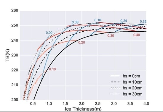
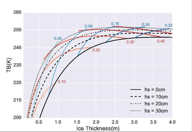
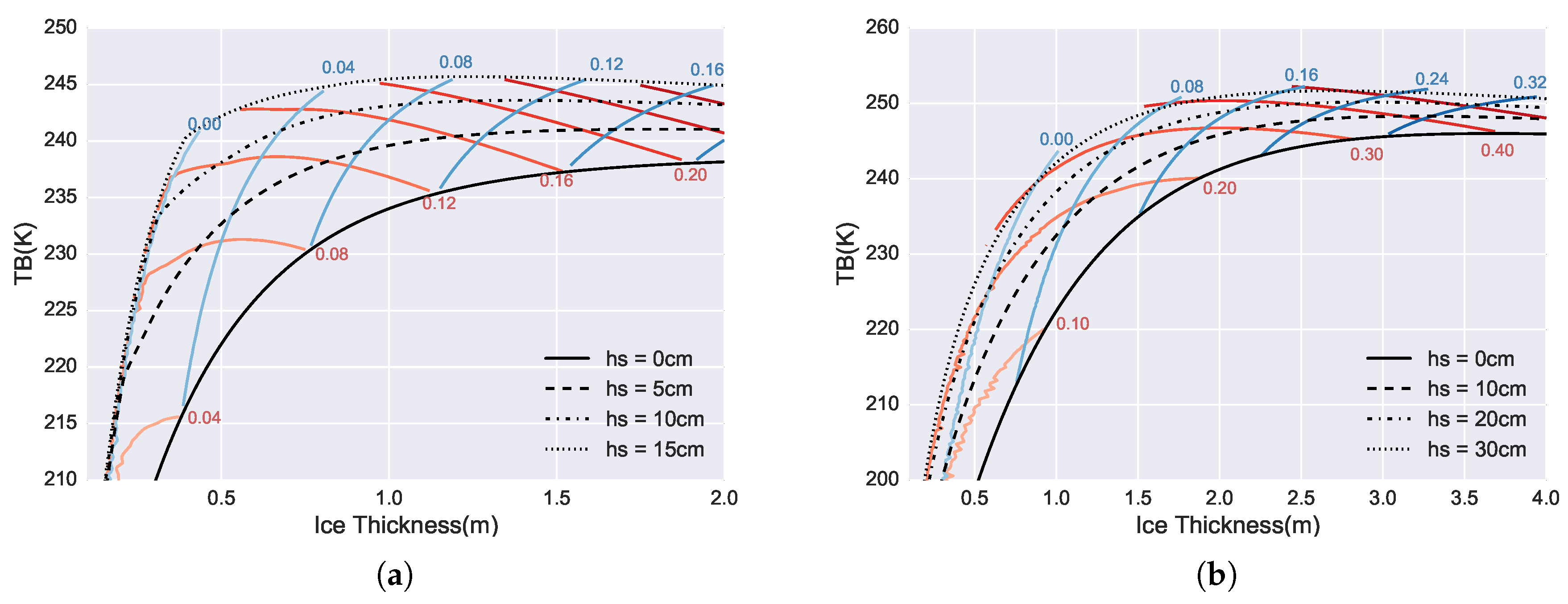
Figure 2 shows the simulated $TB$ with respect to sea ice parameters ($hi$ and $hs$), under normal Arctic winter conditions (the surface temperature of −30 ${}^{\circ }$C). There is non-linear relationship between $TB$ and $hi$ or $hs$. With the deepening of either the sea ice or the snow cover (i.e., increasing $hi$ or $hs$), the value of $TB$ gradually saturates for both FYI and MYI. For $hi$ larger than about 2.5 m (1.2 m) for MYI (FYI), the value of $TB$ saturates. For the retrieval of $hi$ based on a prescribed $hs$, this implies that a small perturbation/error in the observed $TB$ would result in a large difference in the retrieved $hi$, as in Tian-Kunze et al. [22]. Also due to the nonlinear relationship, the retrieval cannot be formulated in an explicit form. We use Equation (1) to represent the nonlinear relationship between $TB$ and related parameters, including: surface temperature ($T_{sfc}$), sea ice type ($ice\_type$), sea water temperature ($T_{water}$) and sea water salinity ($S_{water}$) at the bottom of the sea ice.

$$TB=\mathbf{TB}(hi,hs,T_{sfc},ice\_type,T_{water},S_{water})$$

(1)

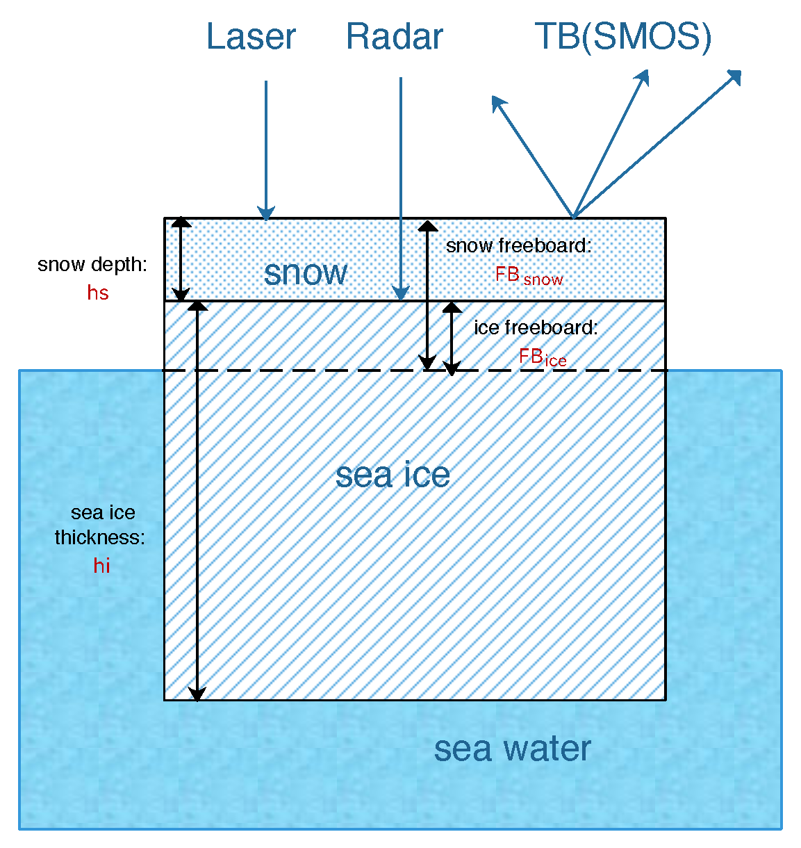
The second physical model as adopted by the retrieval is the hydrostatic equilibrium model based on the buoyancy relationship between $hi$, $hs$ and the density of sea ice, snow and sea water (${\rho }_{ice}$, ${\rho }_{snow}$ and ${\rho }_{water}$). This model is the basis of both radar and laser satellite altimetry [8,10,35]. For radar altimetry as in CryoSat-2 [13,36,37], the sea ice thickness can be estimated with $F{B}_{ice}$ as derived from satellite data, according to Equation (2). For laser altimetry as in ICESat [8,38], the same model is applied with a different form involving $F{B}_{snow}$, as shown in Equation (3).

$$\begin{array}{cc}\hfill hi& =\frac{{\rho }_{water}}{{\rho }_{water}-{\rho }_{ice}}·F{B}_{ice}+\frac{{\rho }_{snow}}{{\rho }_{water}-{\rho }_{ice}}·hs\hfill \end{array}$$

(2)

$$\begin{array}{cc}\hfill hi& =\frac{{\rho }_{water}}{{\rho }_{water}-{\rho }_{ice}}·F{B}_{snow}-\frac{{\rho }_{water}-{\rho }_{snow}}{{\rho }_{water}-{\rho }_{ice}}·hs\hfill \end{array}$$

(3)

Since the linear relationship between $hi$ and $F{B}_{ice}$ or $F{B}_{snow}$, the retrieval of $hi$ can be formulated in the explicit form above. The value of $hs$ is treated as a priori knowledge which can be estimated from other sources (see Section 1).

For the retrieval, we treat $TB$, $F{B}_{ice}$ and $F{B}_{snow}$ as input parameters, and $hi$ and $hs$ the retrieved parameters. Other parameters as used by the models are categorized as model parameters, which are either treated as constants or assumed to be derived from other sources. For the radiation model, $T_{sfc}$ is assumed to be derived from remote sensing or reanalysis data. In this article, we mainly consider the typical winter condition of the Arctic, and the surface temperature is assumed to be −30 ${}^{\circ }$C Besides, we also consider the relatively warmer condition ($T_{sfc}$ = −15 ${}^{\circ }$C) in the sensitivity studies, which is becoming more common with global warming [39]. The values of $T_{water}$ and $S_{water}$ are considered as constants ($T_{water}$ = −1.8 ${}^{\circ }$C and $S_{water}$ = 33 g/kg). Following common practice in satellite altimetry, density values are assumed constant: ${\rho }_{water}$ = 1024 kg/m${}^3$ and ${\rho }_{ice}$ = 915 kg/m${}^3$, as derived from field measurements [40], and ${\rho }_{snow}$ = 320 kg/m${}^3$ following Warren et al. [25]. Although these model parameters are assumed to be constant, the uncertainty as caused by these parameters are all analyzed systematically for the sensitivity studies in Section 4.

With the transformed forms of Equations (2) and (3), we can also derive $F{B}_{ice}$ and $F{B}_{snow}$ based on $hi$ and $hs$. In Figure 2, the colored lines (with labels) represent constant $F{B}_{ice}$ (blue lines) and constant $F{B}_{snow}$ (red lines). Since $F{B}_{ice}$ and $F{B}_{snow}$ are input parameters, the solution to the retrieval based on $TB$ and freeboard synergy resides on the corresponding constant freeboard lines. For the synergy between $TB$ and $F{B}_{ice}$, $TB$ increases monotonically on each constant $F{B}_{ice}$ line, in spite of the saturation and minor decrease of $TB$ with respect to $hi$. This implies good potential of retrieving $hi$ and $hs$ based on $TB$ and $F{B}_{ice}$. However, for the synergy between $TB$ and $F{B}_{snow}$, under certain values of $F{B}_{snow}$ (e.g., 0.12 m for FYI and 0.30 m for MYI), there is no monotonic increase of $TB$ with the increase of $hi$. This implies that for certain combinations of $T{B}_{snow}$ and $TB$, there may exist more than 1 solution to the retrieval problem. It is worth noting that for thick sea ice, there is potentially better sensitivity for both schemes of synergy, as indicated by the non-flat constant freeboard lines with respect to $TB$.

2.2. Retrievability Analysis

We construct the solution space for the retrieval problems by scanning the sea ice parameters. For each scanned values of $hi$ and $hs$, we generate the values of $TB$, $F{B}_{ice}$ and $F{B}_{snow}$. We exclude the cases involving inundation (i.e., $F{B}_{ice}<0$), which is uncommon for Arctic regions. The solution space for each of the data synergy scheme is plotted and examined with respect to the input parameters.

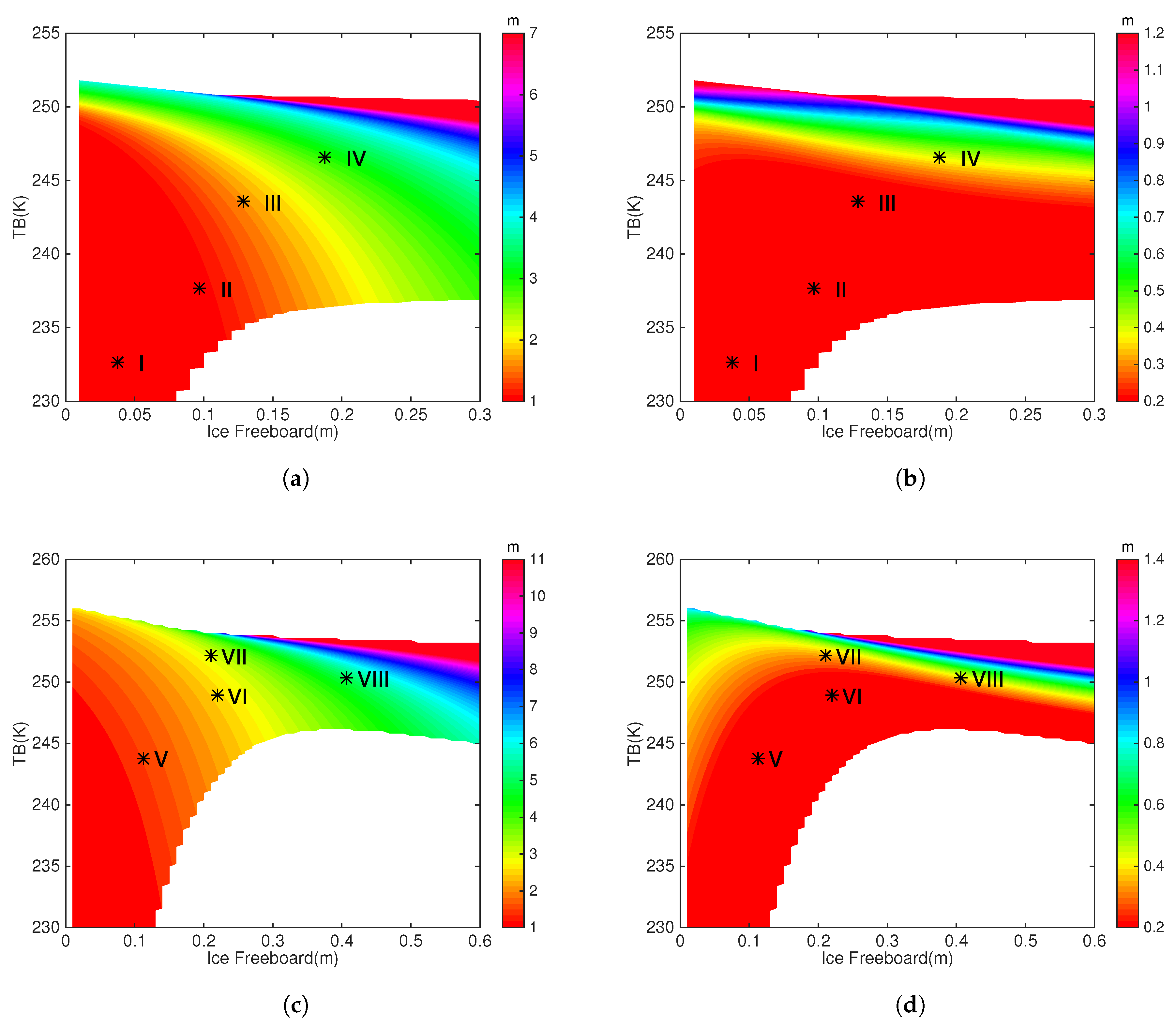
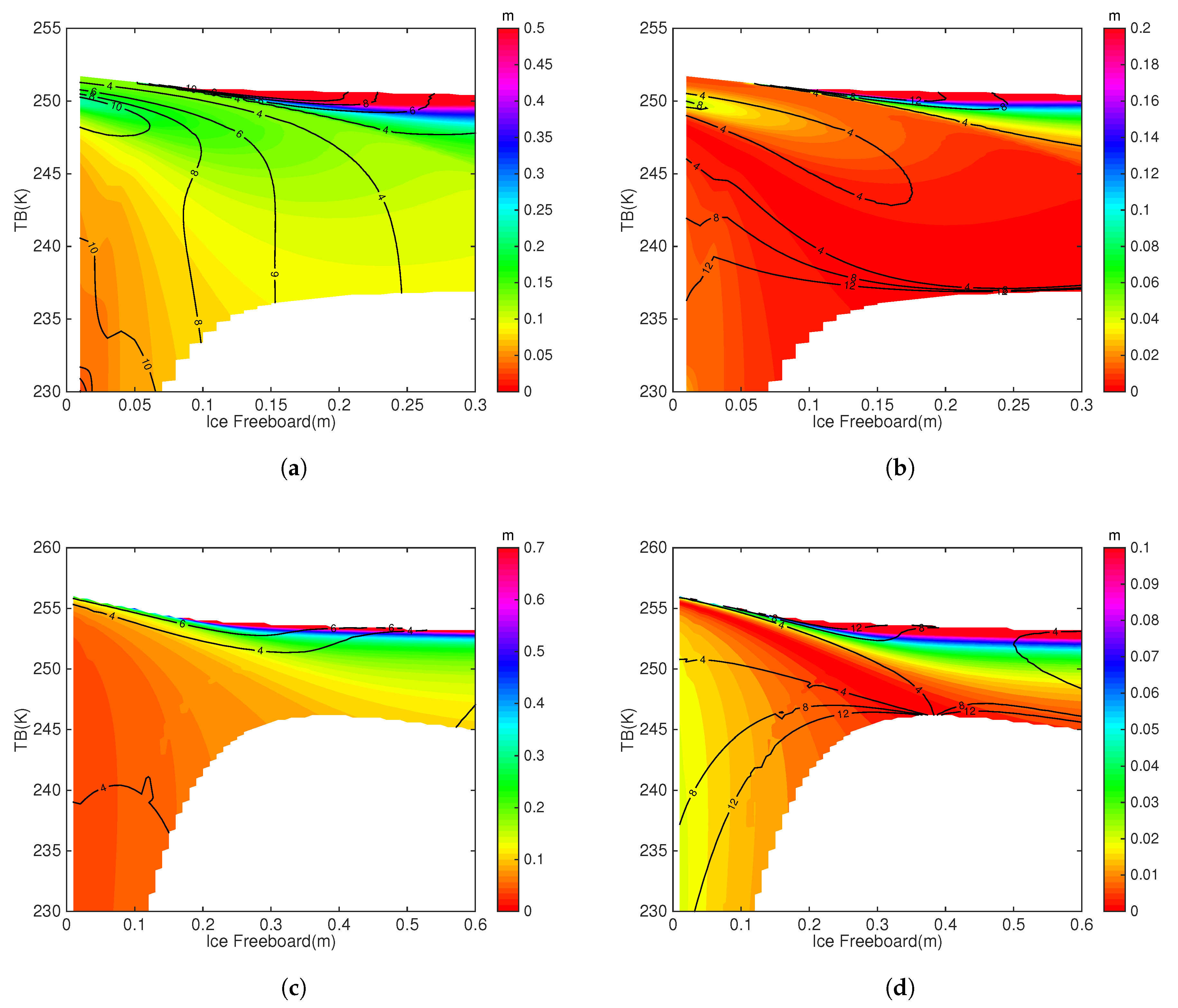
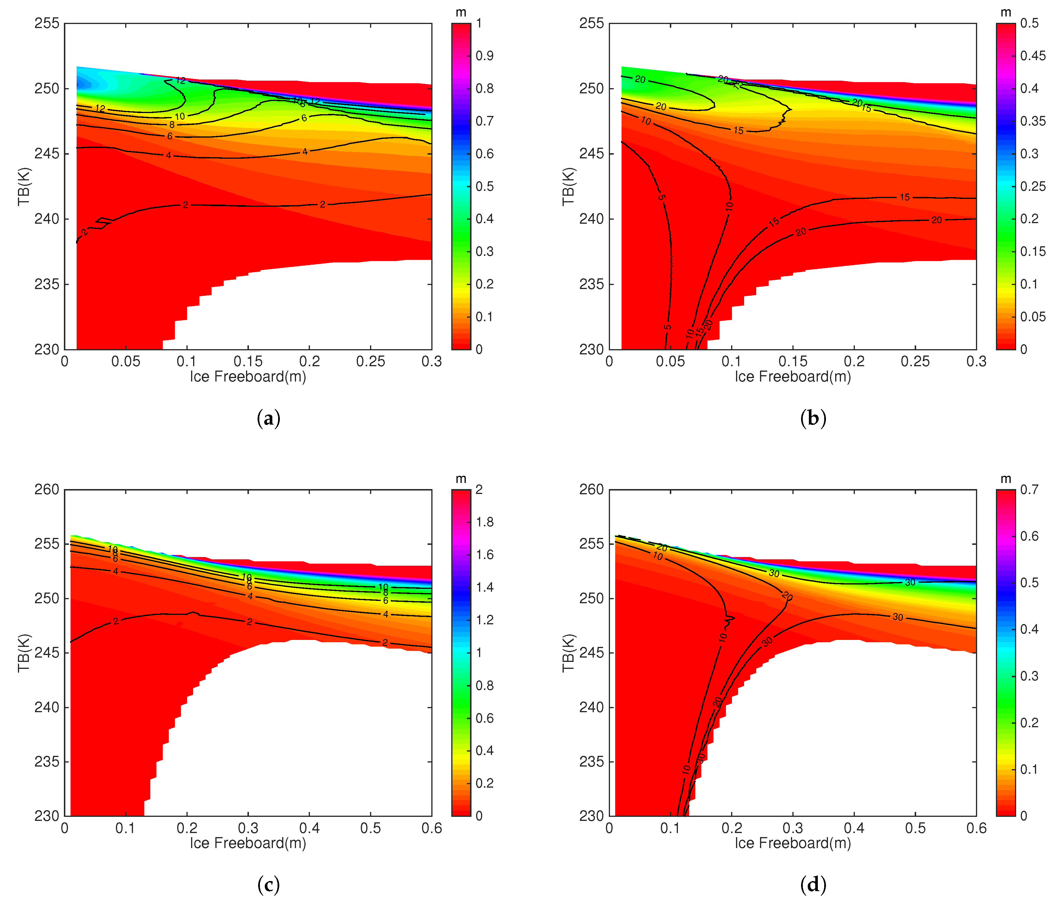
For the synergy between $TB$ and $F{B}_{ice}$, Figure 3a,b show the solution space for $hi$ and $hs$ respectively for FYI, and Figure 3c,d show those for MYI. A reasonable range of the solution space for both $hi$ and $hs$ is included ($hi$ within about 10 m and $hs$ within 1 m). With a certain value of $F{B}_{ice}$, there exists a range of possible $TB$ values. For FYI, with the increase in $F{B}_{ice}$, the lowest possible value of $TB$ also increases. For MYI, there is a slight decrease of the lowest bound of $TB$ when $F{B}_{ice}$ is high. Due to the saturation of $TB$ with respect to either $hi$ or $hs$, there also exists an upper bound for $TB$. Under certain value of $TB$ (or $F{B}_{ice}$), the solutions of both $hi$ and $hs$ become larger with the increase of $F{B}_{ice}$ (or $TB$).

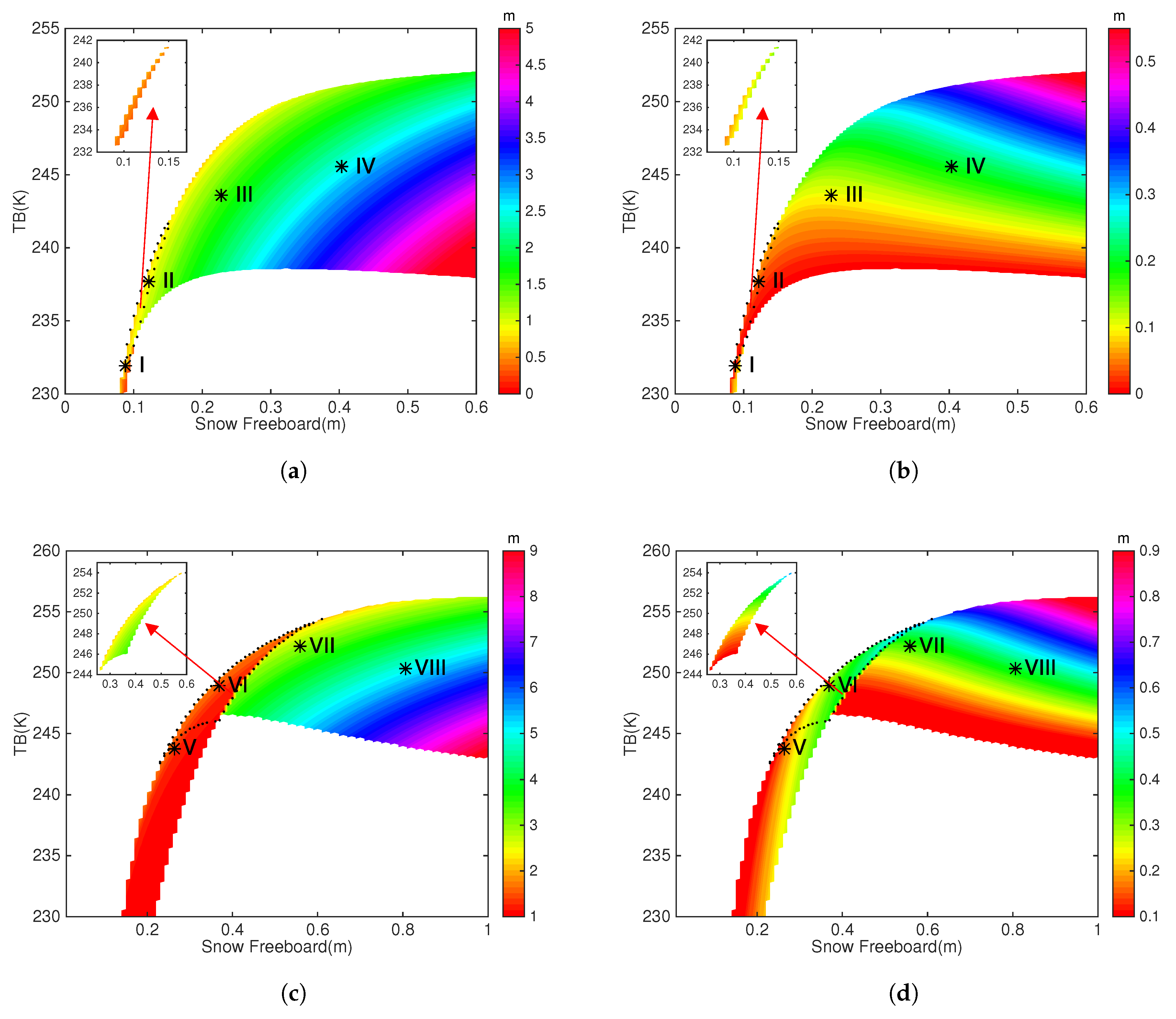
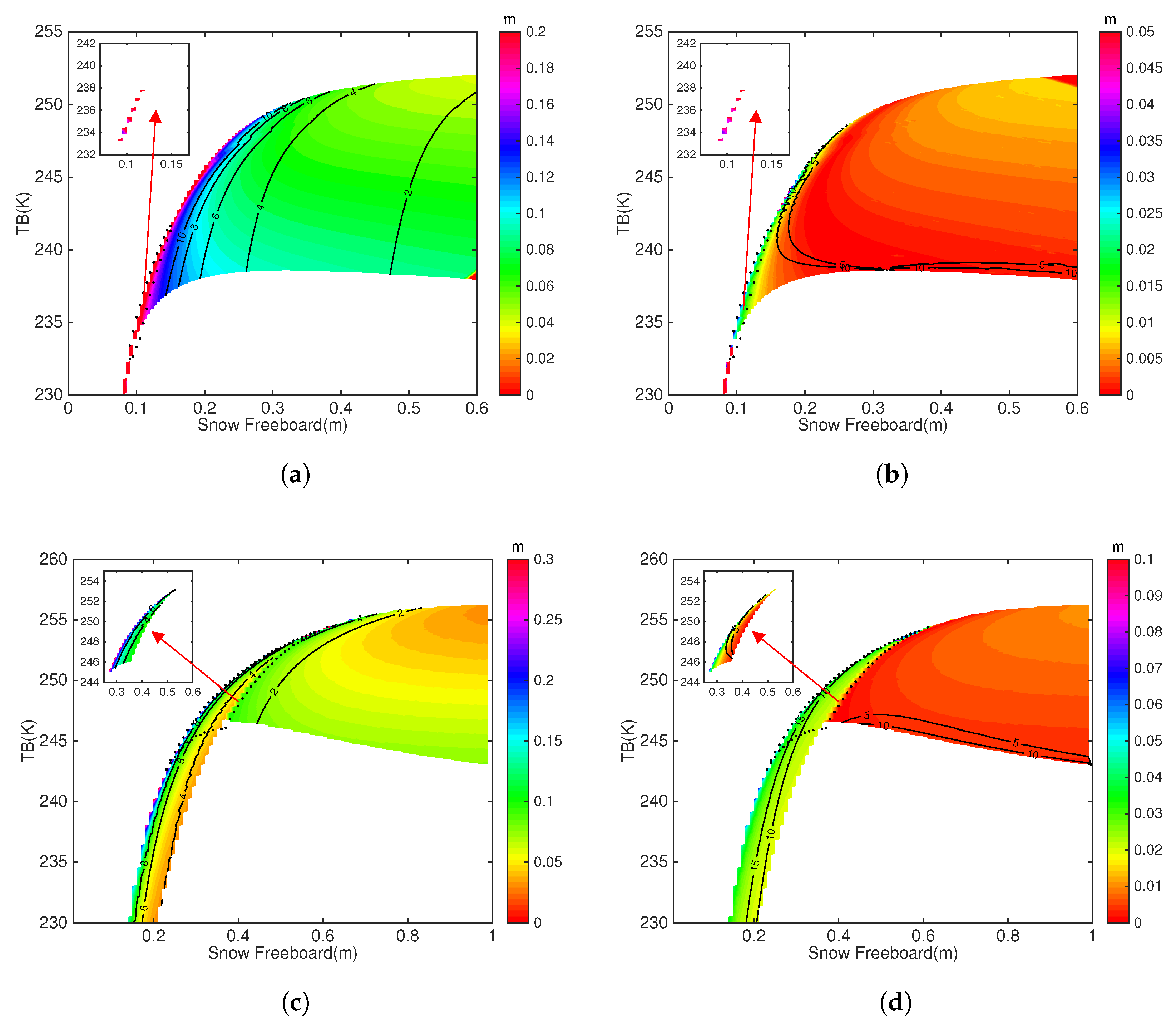
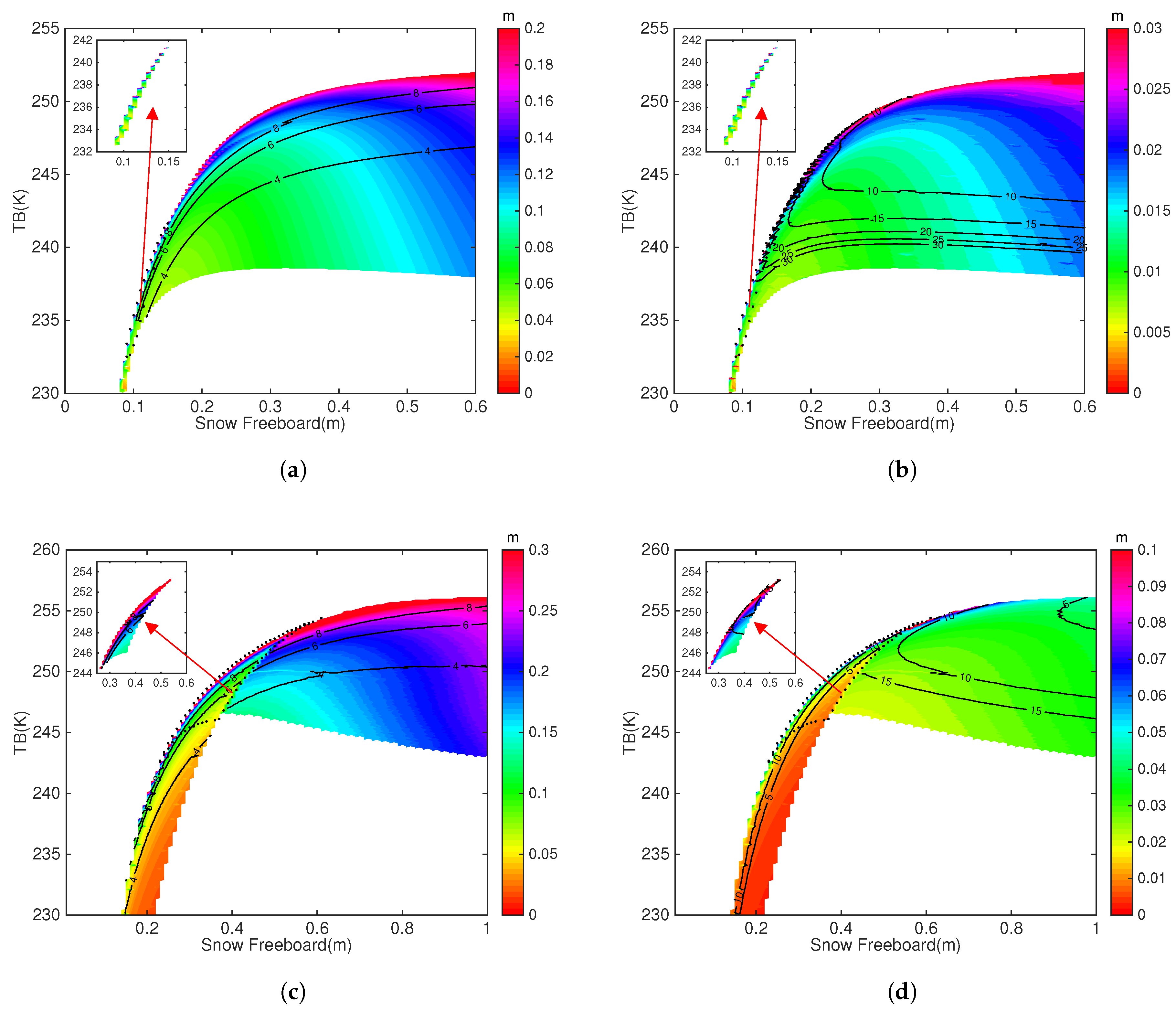
Figure 4 shows the solution space for the synergy between $TB$ and $F{B}_{snow}$. As compared with the corresponding information in Figure 3, there exists evident differences. The most prominent difference from the synergy between $TB$ and $F{B}_{ice}$ is the presence of two potential solutions for certain part of the solution space. Therefore, the retrieval problem of the synergy between $TB$ and $F{B}_{snow}$ is not well-posed. In each subfigure, the portion of the solution space that involves two potential solutions is outlined by dotted lines in the main part. The other solution of this portion of the solution space is also shown by embedded graph in each subfigure. The corresponding input parameters are as follows: (1) for FYI, $F{B}_{snow}$ around 0.1 m and $TB$ around 237 K, (2) for MYI, $F{B}_{snow}$ around 0.37 m and $TB$ around 247 K. For FYI, this portion consists of a small part (3.32%) of the solution space, and the corresponding two solutions for $hi$ ($hs$) are about 0.4 m and 0.9 m (0.1 m and 0.07 m). For MYI, the proportion is higher (6.67%), and the two potential solutions for $hi$ ($hs$) are about 1.3 m and 2.8 m (0.3 m and 0.12 m).

We also consider the relatively warmer Arctic condition with $T_{sfc}$ = −15 ${}^{\circ }$C, instead of the normal winter condition ($T_{sfc}$ = −30 ${}^{\circ }$C). Examination of the corresponding solution space is carried out in a similar manner. The results (not shown) indicate that under the relatively warmer condition, the range of $TB$ is from 247 K to 255 K (250 K to 257 K) when $F{B}_{ice}$ is large in FYI (MYI) algorithm. This range is narrower as compared to winter condition (Figure 3). However, the well-posedness (ill-posedness) of the retrieval problem for the synergy between $TB$ and $F{B}_{ice}$ ($F{B}_{snow}$) is not changed. Besides, the portion of the solution space that involves two solutions takes up about $9.28\%$ ($5.49\%$) for FYI (MYI).

To summarize, there exists retrievability of sea ice parameters with the observational data of L-band $TB$ and freeboard measurements. For typical parameters, both $hi$ and $hs$ can be attained given the combination of $TB$ and $F{B}_{ice}$ or $F{B}_{snow}$. The synergy between $TB$ and $F{B}_{ice}$ is always well-posed, while for that between $TB$ and $F{B}_{snow}$ there is potential of two solutions. These characteristics of the solution space should be accounted for by the retrieval algorithms.

3. Retrieval Algorithms

To accommodate the different characteristics of the data synergy schemes, we construct two retrieval algorithms with the forward physical models. For the synergy between $TB$ and $F{B}_{ice}$, due to the retrieval problem is well-posed, we start with a minimum guess for snow depth ($hs=0$), and the corresponding $hi$ can be computed according to Equation (2). At each iteration, the values of $hi$ and $hs$ are used to compute the TB using the forward radiation model. The modeled TB is compared against the observed TB. If the modeled TB is lower, $hs$ is then increased for the next iteration. Otherwise, a small step in increasing $hs$ is adopted. Therefore an iterative process (involving binary search) is carried out to locate the proper value of $hs$ (as well as $hi$) that generates the observed TB. The outline of the iterative algorithm is shown in Figure 5.

For the synergy between $TB$ and $F{B}_{snow}$, since there exists possibility of two potential solutions, instead of a simple iterative process in Figure 5, two steps are involved for the retrieval. Firstly, a scanning process within the possible range of $hs$ is carried out. The scanning targets at individual values of $hs$ by a sufficiently small step (e.g., 1 cm). Potential solutions are detected when the values of modeled $TB$ from two adjacent values of $hs$ reside on different side of the observed $TB$. For the second step, for each potential solution, a binary search process can then be carried out. For the case involving two potential solutions, both of them are reported by the retrieval algorithm. The outline of this algorithm is shown in Figure 6.

In order to verify the retrieval algorithms, we construct 8 idealized retrieval scenarios that are typical for the Arctic region. As shown in

Table 1. Sea ice parameters ($hi$ and $hs$) and observed parameters ($F{B}_{ice}$, $F{B}_{snow}$ and $TB$) for 8 typical retrieval scenarios for the Arctic.

Ice Type	Scenario	hi (m)	hs (m)	FBice (m)	FBsnow (m)	TB (K)
FYI	I	0.5	0.05	0.0376	0.0876	231.5
	II	1.0	0.03	0.0971	0.1271	238.2
	III	1.5	0.10	0.1284	0.2284	243.7
	IV	2.5	0.25	0.1880	0.4380	246.5
MYI	V	1.5	0.15	0.1127	0.2627	243.8
	VI	2.5	0.15	0.2192	0.3692	248.9
	VII	3.0	0.35	0.2100	0.5600	252.0
	VIII	5.0	0.40	0.4072	0.8072	250.4

, these scenarios cover both sea ice types, as well as a range of sea ice thickness and snow depth. The derived parameters based on physical models in Section 2.1 are also shown, including $F{B}_{ice}$, $F{B}_{snow}$ and L-band $TB$. We denote these scenarios by number I to VIII, and their locations in the solution space for both types of data synergy are indicated in Figure 3 and Figure 4.

We carry out retrieval with the derived values of $F{B}_{ice}$, $F{B}_{snow}$ and L-band $TB$, using the corresponding retrieval algorithm.

Table 2. Retrieved sea ice parameters ($hi$ and $hs$) for typical scenarios in Table 1. For the case with two potential solutions, the bold texts show the true solution, while the red texts in parentheses the other potential solution. The case with double solutions is only possible for the synergy of $TB$ and $F{B}_{snow}$.

Results	Data Synergy	Scenario
		I	II	III	IV	V	VI	VII	VIII
Retrieved $hi$ (m)	$TB$ & $F{B}_{ice}$	0.5000	1.0000	1.5000	2.5000	1.5000	2.5000	3.0000	5.0000
	$TB$ & $F{B}_{snow}$	0.5000	1.0000	1.5000	2.5000	1.5000	2.5000	3.0000	5.0000
			(0.5552)				(1.5499)
True $hi$ (m)		0.50	1.00	1.50	2.50	1.50	2.50	3.00	5.00
Retrieved $hi$ (m)	$TB$ & $F{B}_{ice}$	0.0500	0.0300	0.1000	0.2500	0.1500	0.1500	0.3500	0.4000
	$TB$ & $F{B}_{snow}$	0.0500	0.0300	0.1000	0.2500	0.1500	0.1500	0.3500	0.4000
			(0.0989)				(0.2971)
True $hs$ (m)		0.05	0.03	0.10	0.25	0.15	0.15	0.35	0.40

shows the retrieval results. By comparison with the true values of the parameters, we demonstrate that the true values of $hi$ and $hs$ are attained with both types of data synergy. For the synergy between $TB$ and $F{B}_{ice}$, the retrieval solution is unique for all scenarios. For the synergy between $TB$ and $F{B}_{snow}$, two potential solutions are possible for scenario II and VI. The true solution is included in the retrieval result, and the other solution is shown in red for each scenario. It is further verified this solution does produce the same $F{B}_{snow}$ and $TB$ as the true solution. As compared with the true solution, the snow is thicker and the sea ice is thinner. Consistent with the retrievability study, it is indicated that scenario II and VI are included in the portion of the solution space that contain ambiguous solutions, as in Figure 4.

4. Sensitivity Studies

In this section we carry out sensitivity study over the retrieved parameters and the effect of both the input and the model parameters. We first examine that of input parameters in Section 4.1 and Section 4.2, and further examine that of model parameters in Section 4.3. The uncertainty for these parameters are listed in

Table 3. The uncertainty ($\sigma$) of input parameters and model parameters in sensitivity studies.

Input Parameters
	${\sigma }_{F{B}_{ice}}$ (m)	${\sigma }_{F{B}_{snow}}$ (m)	${\sigma }_{TB}$ (K)
	0.01	0.01	0.5
Model Parameters
${\sigma }_{{\rho }_{ice}}$ (kg/m${}^3$)	${\sigma }_{{\rho }_{snow}}$ (kg/m${}^3$)	${\sigma }_{T_{sfc}}$ (K)	${\sigma }_{T_{water}}$ (K)	${\sigma }_{S_{water}}$ (psu)
10	33.3	1.031	0.2	2

. The values are the in standard deviation ($\sigma$) as derived from typical observations or datasets. For example, the uncertainty of $TB$ is 0.5 K, as specified by SMOS data [22], and the uncertainty of $S_{water}$ represents Arctic basin-wide variability of surface salinity. Therefore, these values serve as references to the uncertainty of the data during actual retrieval practice. Uncertainty in the retrieved parameters are quantified by either differentiation or Monte Carlo simulations with perturbations to both individual parameters and a set of parameters. In Monte-Carlo simulations, all the perturbations to all parameters except the freeboard values follow normal distribution with the prescribed standard deviations. The perturbation to freeboard values ($F{B}_{ice}$ and $F{B}_{snow}$) follow log-normal distributions to avoid negative freeboards. Results show that $TB$ and freeboard plays different roles in the uncertainty of $hi$ and that of $hs$. Furthermore, model parameters play a non-negligible role as compared with input parameters. For further study with realistic data, both types of parameters should be accounted for the uncertainty estimation of the retrieved parameters.

4.1. Effect of Input Parameters for the Synergy between $TB$ and $F{B}_{ice}$

Based on the solution spaces of both types of data synergy, we compute the differences of the retrieved $hi$ and $hs$ as caused by perturbations to either $TB$ or freeboard values. First, we compute the absolute uncertainty of $hi$ and $hs$, denoted ${ϵ}_{absolute}$:${ϵ}_{absolute}{|}_y=\frac{{\Delta }_y}{{\Delta }_x}·{\sigma }_x$, where x is the input parameter ($TB$ or $F{B}_{ice}$ or $F{B}_{snow}$), and y the retrieved parameter ($hi$ or $hs$). The values of ${\Delta }_x$ and ${\Delta }_y$ are derived by differentiation within the solution space in Figure 3 and Figure 4, and the value of $\frac{{\Delta }_y}{{\Delta }_x}$ characterizes the rate of change in y as caused by a small perturbation in x. Therefore ${ϵ}_{absolute}$ represents the uncertainty of y in terms of standard deviation. Second, we compute the relative uncertainty based on the absolute uncertainty and the actual value of the parameter. The relative uncertainty is defined as: ${ϵ}_{relative}{|}_y=\frac{{ϵ}_{absolute}{|}_y}{y}\times 100\%$, which is the percentage of the uncertainty of y with respect to y.

For the data synergy between $TB$ and $F{B}_{ice}$, Figure 7 and Figure 8 show the uncertainty analysis for perturbations to $F{B}_{ice}$ and $TB$, respectively. As shown in Figure 7, the uncertainty in $hi$ as caused by that of $F{B}_{ice}$ is generally lower than 10% (subfigure a and c). For comparison, as in Figure 8, the uncertainty in $hi$ as caused by $TB$ is generally lower than that caused by $F{B}_{ice}$ when $TB$ is relatively low. However, when $TB$ is high ($hi$ > 4 m and $hs$ > 0.9 m for FYI, or $hi$ > 7 m and $hs$ > 70 cm for MYI), the uncertainty as caused by $TB$ is larger than that of $F{B}_{ice}$. This change is attributed to the saturation feature of $TB$ for thick ice. It is worth noting that these parameters are relatively rare during Arctic observations. For $hs$, when comparing Figure 7 and Figure 8, it is shown that different from the case of $hi$, $TB$ always plays a dominant role in the uncertainty of $hs$. The uncertainty in $hs$ as caused by $F{B}_{ice}$ is only higher than 10% when $TB$ is lower than about 238 K or higher than 250 K for FYI, and lower than 246 K or higher than 253% for MYI. However, $TB$ consistently causes nearly 10% or higher uncertainty in $hs$ for both FYI and MYI. As a result, $TB$ causes larger uncertainty in $hs$ for a larger portion of the solution space than $F{B}_{ice}$. Similar to $hi$, when both $hi$ and $hs$ are relatively large, there exists increase in the uncertainty of $hs$ for both absolute and relative terms (>0.4 m or 20% for FYI, and >0.5 m or 30% for MYI).

We further carry out sensitivity studies for the 8 typical retrieval scenarios as introduced in Section 3. In order to evaluate the uncertainty in the retrieved $hi$ and $hs$, we apply Monte Carlo simulations with the retrieval algorithms. For each type of data synergy, three simulations are carried out, containing random perturbations to the value of freeboard, to that of $TB$, and to both of them. Each simulation contains 5000 samples. Each simulation sample contains a perturbation (or a set of perturbations), and the retrieval is carried out with the perturbed parameter(s). Perturbations follow normal distribution for $TB$ and log-normal distribution for freeboard (see Table 3). The uncertainty in the retrieved $hi$ and $hs$ is then estimated by computing the standard deviation among the samples.

Table 4. Relative uncertainty (units: %) in the retrieved $hi$ and $hs$ for the synergy between $TB$ and $F{B}_{ice}$, as estimated by Monte-Carlo simulations. Normal Arctic winter condition is assumed (surface temperature of −30 ${}^{\circ }$C). In each Monte-Carlo simulation sample, the retrieval process is carried out with a random perturbation to the designated parameter(s). The perturbations are Gaussian, with the standard deviation in Table 3. The relative uncertainty ${ϵ}_{relative}{|}_y$ is given by: $\frac{{\sigma }_y}{y}\times 100\%$, where ${\sigma }_y$ is the standard deviation of y estimated from samples of the corresponding Monte-Carlo simulation, and y the true value (y for $hi$ or $hs$). Sensitivity studies are carried out for each input or model parameter, each set of parameters, as well as all parameters (in different columns). The numbers in bold are the relatively larger one between the two values associated with the input parameters.

Scenario	Results	${\mathit{FB}}_{\mathit{ice}}$	$\mathit{TB}$	Both Input Param.	${\mathit{\rho }}_{\mathit{ice}}$	${\mathit{\rho }}_{\mathit{snow}}$	${\mathit{T}}_{\mathit{sfc}}$	All Model Param.	All Param.
I	$hi$	$\mathbf{11.18}\%$	$1.15\%$	$10.69\%$	$3.93\%$	$0.72\%$	$1.52\%$	$4.39\%$	$11.50\%$
	$hs$	$\mathbf{27.61}\%$	$3.91\%$	$26.73\%$	$10.27\%$	$5.60\%$	$5.17\%$	$13.10\%$	$29.55\%$
II	$hi$	$\mathbf{7.79}\%$	$1.18\%$	$7.93\%$	$5.92\%$	$0.10\%$	$1.64\%$	$6.16\%$	$9.85\%$
	$hs$	$\mathbf{18.45}\%$	$13.42\%$	$23.24\%$	$13.95\%$	$8.28\%$	$18.61\%$	$25.16\%$	$33.80\%$
III	$hi$	$\mathbf{6.74}\%$	$2.39\%$	$7.08\%$	$7.71\%$	$0.53\%$	$2.54\%$	$8.24\%$	$11.24\%$
	$hs$	$2.23\%$	$\mathbf{12.22}\%$	$12.40\%$	$2.77\%$	$5.55\%$	$12.95\%$	$14.52\%$	$20.21\%$
IV	$hi$	$\mathbf{4.75}\%$	$3.92\%$	$6.27\%$	$9.29\%$	$1.31\%$	$3.54\%$	$10.04\%$	$11.73\%$
	$hs$	$3.54\%$	$\mathbf{13.36}\%$	$13.72\%$	$6.75\%$	$4.03\%$	$12.06\%$	$14.67\%$	$20.05\%$
V	$hi$	$\mathbf{3.71}\%$	$1.62\%$	$3.96\%$	$4.10\%$	$1.23\%$	$1.79\%$	$4.45\%$	$5.98\%$
	$hs$	$\mathbf{9.67}\%$	$5.41\%$	$10.55\%$	$10.69\%$	$5.12\%$	$5.99\%$	$12.93\%$	$16.49\%$
VI	$hi$	$\mathbf{3.21}\%$	$2.16\%$	$3.77\%$	$6.12\%$	$0.58\%$	$1.96\%$	$6.48\%$	$7.75\%$
	$hs$	$3.85\%$	$\mathbf{12.28}\%$	$12.52\%$	$6.38\%$	$5.49\%$	$11.10\%$	$13.77\%$	$18.95\%$
VII	$hi$	$3.88\%$	$\mathbf{6.22}\%$	$7.36\%$	$10.13\%$	$1.55\%$	$3.69\%$	$12.65\%$	$16.59\%$
	$hs$	$2.66\%$	$\mathbf{18.18}\%$	$18.54\%$	$8.54\%$	$3.96\%$	$10.78\%$	$18.97\%$	$33.30\%$
VIII	$hi$	$3.21\%$	$\mathbf{6.40}\%$	$7.13\%$	$12.83\%$	$1.35\%$	$4.38\%$	$15.32\%$	$18.03\%$
	$hs$	$5.66\%$	$\mathbf{27.24}\%$	$27.80\%$	$23.34\%$	$4.12\%$	$18.63\%$	$34.59\%$	$50.31\%$

(first 3 columns of the results) shows the relative uncertainty as estimated from the simulations for the synergy between $TB$ and $F{B}_{ice}$. The relative uncertainty of parameter y, denoted ${ϵ}_{relative}{|}_y$ is computed as $\frac{{\sigma }_y}{y}\times 100\%$, where ${\sigma }_y$ is the standard deviation as derived from Monte-Carlo samples and y the true value of the parameter. In order to contrast the relative importance between $TB$ and $F{B}_{ice}$, the larger value is shown in bold. For both $hi$ and $hs$, $F{B}_{ice}$ plays an more dominant role or relative thin ice (scenario I, II and V), and $TB$ plays an more important role for thick MYI (scenario VII and VIII). For other scenarios (III, IV, VI), $F{B}_{ice}$ plays a dominant role for $hi$, but $TB$ caused higher uncertainty for $hs$. Also the uncertainty in $hi$ and $hs$ as caused by both input parameters is lower than 11% and 28%, respectively. Besides, they are generally lower than the combined values as caused by each parameter under the assumption of independence. This implies that the uncertainty in $hi$ and $hs$ is correlated, although the uncertainty in input parameters are independent.

Aside from the normal winter condition of the Arctic, we also consider a relatively warm condition ($T_{sfc}$=−15 ${}^{\circ }C$), to reflect the effect of global warming for the typical scenarios. The uncertainty is estimated with Monte-Carlo simulations, and the results are shown in

Table 5. Same as Table 4 but for the relatively warm Arctic conditions (surface temperature of −15${}^{\circ }$C).

Scenario	Results	${\mathit{FB}}_{\mathit{ice}}$	$\mathit{TB}$	Both Input Param.	${\mathit{\rho }}_{\mathit{ice}}$	${\mathit{\rho }}_{\mathit{snow}}$	${\mathit{T}}_{\mathit{sfc}}$	All Model Param.	All Param.
I	$hi$	$\mathbf{11.88}\%$	$1.93\%$	$11.48\%$	$4.23\%$	$0.20\%$	$3.53\%$	$5.66\%$	$12.80\%$
	$hs$	$\mathbf{25.35}\%$	$6.56\%$	$25.18\%$	$9.29\%$	$7.81\%$	$12.02\%$	$17.39\%$	$30.68\%$
II	$hi$	$\mathbf{7.45}\%$	$2.20\%$	$7.78\%$	$5.65\%$	$0.71\%$	$3.37\%$	$6.68\%$	$10.13\%$
	$hs$	$22.14\%$	$\mathbf{24.92}\%$	$33.74\%$	$16.77\%$	$16.92\%$	$38.29\%$	$44.08\%$	$54.91\%$
III	$hi$	$\mathbf{6.07}\%$	$5.24\%$	$7.97\%$	$6.91\%$	$1.41\%$	$4.92\%$	$8.71\%$	$12.52\%$
	$hs$	$1.37\%$	$\mathbf{26.78}\%$	$26.76\%$	$1.56\%$	$15.81\%$	$25.13\%$	$30.02\%$	$43.55\%$
IV	$hi$	$4.16\%$	$\mathbf{8.81}\%$	$9.80\%$	$8.21\%$	$1.85\%$	$6.68\%$	$11.10\%$	$15.36\%$
	$hs$	$1.58\%$	$\mathbf{30.01}\%$	$29.73\%$	$3.19\%$	$14.83\%$	$22.75\%$	$28.72\%$	$44.01\%$
V	$hi$	$\mathbf{3.42}\%$	$2.37\%$	$4.17\%$	$3.87\%$	$0.48\%$	$3.14\%$	$5.04\%$	$6.73\%$
	$hs$	$\mathbf{9.84}\%$	$8.11\%$	$12.65\%$	$11.06\%$	$6.65\%$	$10.70\%$	$16.96\%$	$21.27\%$
VI	$hi$	$3.46\%$	$\mathbf{5.93}\%$	$6.86\%$	$6.88\%$	$0.67\%$	$4.63\%$	$8.67\%$	$16.50\%$
	$hs$	$1.59\%$	$\mathbf{33.68}\%$	$33.49\%$	$3.25\%$	$11.64\%$	$26.30\%$	$30.62\%$	$71.31\%$
VII	$hi$	$4.85\%$	$\mathbf{54.97}\%$	$56.27\%$	$14.36\%$	$2.04\%$	$12.50\%$	$32.46\%$	$86.22\%$
	$hs$	$5.17\%$	$>\mathbf{100}\%$	>100%	$19.32\%$	$13.48\%$	$36.50\%$	$76.16\%$	>100%
VIII	$hi$	$3.07\%$	$\mathbf{14.08}\%$	$14.77\%$	$11.86\%$	$1.36\%$	$9.26\%$	$17.23\%$	$28.86\%$
	$hs$	$5.04\%$	$\mathbf{59.97}\%$	$61.86\%$	$19.64\%$	$13.64\%$	$39.41\%$	$51.66\%$	>100%

. Comparison with Table 4 shows that there is little change or slight increase in the uncertainty caused by $F{B}_{ice}$, but the increase in that caused by $TB$ is much larger. In relative terms, $TB$ has become the dominant source of uncertainty of $hi$ for scenario IV and VI, and that of $hs$ for scenario II. With the warmer condition, the saturation of $TB$ with respect to sea ice parameters is more premature, which is the reason for the increase of its role in the uncertainty of the retrieved parameters.

4.2. Effect of Input Parameters for the Synergy between $TB$ and $F{B}_{snow}$

We carry out sensitivity study for the data synergy between $TB$ and $F{B}_{snow}$ as in Section 4.1. On the solution space, the most prominent difference from the synergy between $TB$ and $F{B}_{ice}$ is the region with two potential solutions. In Figure 9 and Figure 10, the sensitivity of the retrieved parameters to $F{B}_{snow}$ and $TB$ in the solution space are shown, respectively. The sensitivity for the portion that contains two potential solutions are shown by embedded figures, similar to Figure 4. For scenario II and IV with two potentials solutions, the effect of double solution is accounted for during the uncertainty estimation. Both $F{B}_{snow}$ and $TB$ have direct influence over the retrieved $hi$ and $hs$. When the sea ice is thin, the relative uncertainty in $hi$ as caused by $F{B}_{snow}$ grows to over 15% for both FYI and MYI. When the sea ice thickness is high, this value drops under 2%. Similar situation applies to $hs$, for shallower snow cover or thinner sea ice, the relative uncertainty as caused by $F{B}_{snow}$ is high. For comparison, the effects of $TB$ is relatively more dominant that of $F{B}_{snow}$ than the data synergy of $F{B}_{ice}$ and $TB$. The influence on the uncertainty of $hs$ is more prominent. For FYI, when $TB$ is low, the relative uncertainty of $hs$ rises up to 20%, and for MYI, to over 15%.

Table 6. Same as Table 4 but for the data synergy between $TB$ and $F{B}_{snow}$.

Scenario	Results	${\mathit{FB}}_{\mathit{ice}}$	$\mathit{TB}$	Both Input Param.	${\mathit{\rho }}_{\mathit{ice}}$	${\mathit{\rho }}_{\mathit{snow}}$	${\mathit{T}}_{\mathit{sfc}}$	All Model Param.	All Param.
I	$hi$	32.96%	35.71%	33.14%	32.90%	37.12%	34.51%	33.24%	33.61%
	$hs$	$\mathbf{61.79}\%$	$60.40\%$	$61.92\%$	$54.80\%$	$62.52\%$	$57.54\%$	$57.13\%$	$62.04\%$
II	$hi$	$\mathbf{28.11}\%$	$24.30\%$	$28.79\%$	$28.10\%$	$24.81\%$	$24.95\%$	$28.48\%$	$29.83\%$
	$hs$	$54.03\%$	$\mathbf{55.47}\%$	$57.48\%$	$54.53\%$	$51.12\%$	$56.77\%$	$58.72\%$	$64.14\%$
III	$hi$	$\mathbf{5.60}\%$	$4.30\%$	$6.98\%$	$6.23\%$	$3.50\%$	$4.60\%$	$8.61\%$	$11.31\%$
	$hs$	$1.75\%$	$\mathbf{9.99}\%$	$10.08\%$	$2.08\%$	$4.59\%$	$10.69\%$	$11.84\%$	$16.09\%$
IV	$hi$	$2.43\%$	$\mathbf{4.34}\%$	$4.90\%$	$4.69\%$	$3.46\%$	$3.91\%$	$7.08\%$	$8.61\%$
	$hs$	$1.96\%$	$\mathbf{6.71}\%$	$6.83\%$	$3.78\%$	$1.86\%$	$6.06\%$	$7.28\%$	$10.28\%$
V	$hi$	$18.67\%$	$\mathbf{22.35}\%$	$22.43\%$	$20.13\%$	$13.16\%$	$22.92\%$	$23.19\%$	$24.56\%$
	$hs$	$38.84\%$	$\mathbf{40.67}\%$	$45.13\%$	$43.55\%$	$21.27\%$	$42.70\%$	$46.33\%$	$46.04\%$
VI	$hi$	$25.31\%$	$\mathbf{26.60}\%$	$27.49\%$	$27.18\%$	$25.27\%$	$26.33\%$	$29.40\%$	$30.88\%$
	$hs$	$35.56\%$	$\mathbf{37.84}\%$	$39.19\%$	$36.18\%$	$35.95\%$	$37.14\%$	$40.38\%$	$43.25\%$
VII	$hi$	$2.26\%$	$\mathbf{7.01}\%$	$7.26\%$	$4.97\%$	$4.32\%$	$4.60\%$	$8.02\%$	$10.54\%$
	$hs$	$1.59\%$	$\mathbf{9.30}\%$	$9.81\%$	$3.02\%$	$2.36\%$	$6.01\%$	$7.17\%$	$11.70\%$
VIII	$hi$	$0.99\%$	$\mathbf{3.99}\%$	$4.16\%$	$3.58\%$	$2.38\%$	$2.93\%$	$5.29\%$	$6.68\%$
	$hs$	$1.74\%$	$\mathbf{7.73}\%$	$7.98\%$	$6.31\%$	$1.25\%$	$5.67\%$	$8.75\%$	$11.63\%$

(first 3 columns) lists the uncertainty estimation for representative scenarios, which is in direct comparison with Table 4. The relative uncertainty as caused by both input parameters drops with the increase in sea ice thickness and snow depth. As contrast from Table 4, $TB$ causes a larger portion of the uncertainty in both $hi$ and $hs$ (6 for $hi$ and 7 for $hs$, among 8 scenarios), while $F{B}_{snow}$ and $TB$ cause uncertainty in $hi$ and $hs$ on equal terms for thin FYI and thin MYI.

When compared with the data synergy between $TB$ and $F{B}_{ice}$, the major difference is that for relatively thinner sea ice, the synergy between $TB$ and $F{B}_{ice}$ yields lower uncertainty in sea ice parameters, and for thicker ice, that between $TB$ and $F{B}_{snow}$ shows advantage. We also carry out the study for these scenarios under relatively warm Arctic conditions (shown in

Table 7. Same as Table 5 but for the data synergy between $TB$ and $F{B}_{snow}$.

Scenario	Results	${\mathit{FB}}_{\mathit{ice}}$	$\mathit{TB}$	Both Input Param.	${\mathit{\rho }}_{\mathit{ice}}$	${\mathit{\rho }}_{\mathit{snow}}$	${\mathit{T}}_{\mathit{sfc}}$	All Model Param.	All Param.
I	$hi$	$\mathbf{22.72}\%$	$21.43\%$	$24.07\%$	$19.07\%$	$20.41\%$	$22.45\%$	$22.81\%$	$26.71\%$
	$hs$	$33.59\%$	$\mathbf{39.53}\%$	$38.73\%$	$38.04\%$	$38.80\%$	$33.12\%$	$34.10\%$	$40.09\%$
II	$hi$	$\mathbf{35.11}\%$	$31.87\%$	$36.07\%$	$32.50\%$	$30.59\%$	$33.18\%$	$36.70\%$	$38.70\%$
	$hs$	$\mathbf{65.16}\%$	$57.95\%$	$63.67\%$	$57.63\%$	$58.09\%$	$54.32\%$	$57.42\%$	$59.10\%$
III	$hi$	$22.46\%$	$\mathbf{26.36}\%$	$27.92\%$	$11.34\%$	$25.48\%$	$20.72\%$	$29.56\%$	$30.48\%$
	$hs$	$33.11\%$	$\mathbf{43.44}\%$	$42.57\%$	$16.17\%$	$38.12\%$	$41.13\%$	$44.20\%$	$47.93\%$
IV	$hi$	$3.02\%$	$\mathbf{13.61}\%$	$13.57\%$	$5.57\%$	$10.65\%$	$10.42\%$	$15.63\%$	$19.12\%$
	$hs$	$1.14\%$	$\mathbf{20.55}\%$	$20.21\%$	$2.12\%$	$12.17\%$	$16.45\%$	$19.73\%$	$26.72\%$
V	$hi$	$18.29\%$	$\mathbf{22.08}\%$	$22.64\%$	$18.82\%$	$20.58\%$	$22.93\%$	$24.64\%$	$25.65\%$
	$hs$	$45.23\%$	$\mathbf{47.91}\%$	$49.65\%$	$48.24\%$	$44.07\%$	$46.84\%$	$49.28\%$	$47.62\%$
VI	$hi$	$25.35\%$	$\mathbf{29.36}\%$	$29.88\%$	$26.29\%$	$25.77\%$	$28.88\%$	$30.74\%$	$33.50\%$
	$hs$	$34.60\%$	$\mathbf{40.92}\%$	$41.90\%$	$34.23\%$	$35.37\%$	$40.10\%$	$42.10\%$	$47.46\%$
VII	$hi$	$1.74\%$	$\mathbf{12.16}\%$	$12.29\%$	$3.94\%$	$6.80\%$	$8.03\%$	$12.49\%$	$16.36\%$
	$hs$	$1.79\%$	$\mathbf{16.01}\%$	$15.85\%$	$4.06\%$	$5.40\%$	$10.75\%$	$13.04\%$	$19.90\%$
VIII	$hi$	$1.03\%$	$\mathbf{7.99}\%$	$7.80\%$	$3.77\%$	$3.83\%$	$6.63\%$	$8.67\%$	$11.62\%$
	$hs$	$1.69\%$	$\mathbf{15.37}\%$	$14.99\%$	$6.19\%$	$3.80\%$	$13.04\%$	$14.58\%$	$21.29\%$

). For relatively thinner sea ice cover, there is no general trend of the uncertainty in the retrieved parameters. However, for scenarios with thicker ice, the relative uncertainty as caused by $TB$ generally double or triple. Similar to the other type of synergy, the uncertainty caused by freeboard measurements stays unchanged, due to the irrelevance of the physical model of buoyancy to the change of temperature from −30 ${}^{\circ }$C to −15 ${}^{\circ }$C.

4.3. Uncertainty Analysis from Model Parameters

Apart from input parameters, the effect of model parameters on the retrieved sea ice parameters are evaluated in terms of uncertainty. We extend the Monte-Carlo simulations in Section 4.1 and Section 4.2 to include perturbations to model parameters. The analyzed parameters are listed in Table 3. Since the effects of $T_{water}$ and $S_{water}$ are very small, causing less than 0.01% change in the retrieved $hi$ and $hs$. This is due to two reasons: (1) they have very small impact on the density of the water and the corresponding retrieval process of altimetry, and (2) the radiative properties of the sea ice covered ocean are dominated by that of the sea ice cover, and the small change in the radiative property of the sea water as caused by these parameters has little impact on the sea ice retrieval. Therefore, we focus on the other 3 parameters: ${\rho }_{ice}$, ${\rho }_{snow}$ and $T_{sfc}$. The density values mainly affect the physical model for altimetry, influencing the quantitative relationship between $hi$ and $hs$ under a linear relationship (see Equations (2) and (3)). Due to the observed large uncertainty and seasonal evolution of ${\rho }_{snow}$ [25] as well as their important role in altimetry [41,42], their uncertainty values are chosen accordingly to reflect their change during the Arctic winter season, ranging from 220 kg/m${}^3$ to 420 kg/m${}^3$ (see also [43,44]). The uncertainty of ${\rho }_{ice}$ is set to 10 kg/m${}^3$, after [41,43,44]. On the other hand, $T_{sfc}$ mainly affects the retrieval results through its influence over the vertical temperature structure of the sea ice cover and its radiative properties [32]. The uncertainty of $T_{sfc}$ of about 1 K is derived from OIB dataset [45], which reflects the variability of surface temperature within a range of 25 km which is commonly used for the production of polar remote sensing data products.

In Table 4, Table 5, Table 6 and Table 7, the uncertainty as caused by ${\rho }_{ice}$, ${\rho }_{snow}$, $T_{sfc}$, and their combination are shown in column 4 to 7 (of the results). When compared with input parameters, they show non-negligible influence over the uncertainty of retrieved parameters. Their combined effect is comparable to that of input parameters across all scenarios. Besides, for the synergy between $TB$ and $F{B}_{ice}$, with the increase of $hi$ and $hs$, the uncertainty caused by these model parameters increase, but for the synergy between $TB$ and $F{B}_{snow}$, the decrease of the uncertainty for $hi$ and $hs$ is witnessed. This is in general consistency with the analysis for input parameters, and coincides with the relative advantage of the two types of synergy over different range of sea ice parameter. Under warmer conditions, the difference as caused by density values generally remain unchanged, while that of $T_{sfc}$ increase by 100% or higher for both $hi$ and $hs$.

For the uncertainty estimation of the typical scenarios, we also produce a set of Monte-Carlo simulation that contain perturbations to all the parameters (including both input and model parameters), as shown by the last column in each table. For the retrieval problem, the model parameters are mainly derived from other supportive data sources, and not directly provided by satellite altimetry or L-band remote sensing data. However, according to the analyses, they can have equally profound influence over the retrieved parameters, which is consistent with existing studies such as the analysis of satellite altimetry [41,42]. Their effect should also be accounted for during the actual retrieval problems for the data synergy proposed by this article.

5. Verification with OIB and SMOS Data

5.1. Data

For the verification, we use airborne measurements from OIB and SMOS satellite based TB data, by considering the co-registered scanning of the sea ice by the two independent data sets. OIB data are provided as 40 m resolution along-track scanning of the sea ice cover. The onboard snow radar and laser altimeter measure the nadir snow depth and total freeboard, and the sea ice thickness can be derived with these parameters. All the data from OIB campaigns during year 2012 and 2015 are used for the retrieval and verifications [34]. The level-4 SMOS TB data product [46] is adopted, which are regridded on the 12.5 km EASE grid.

SMOS TB field on the same date of each OIB campaign is attained for the data synergy. Due to the inherent resolution difference between OIB (limited swath) and SMOS, we treat OIB as samples of the underlying sea ice cover that corresponds to a single TB value in the daily SMOS TB field. Although the resolution of the SMOS TB product is 12.5 km, the native resolution of SMOS measurements is about 40 km. Therefore, all the measurements from OIB that are within the 9 EASE grid cells are treated as samples, covering an area of 37.5 km × 37.5 km which is consistent in general with the native resolution of SMOS measurements.

For the verification, we align the spatial resolution of OIB data to that of SMOS. Points with mixed sea ice type, open water or lead are excluded for further retrieval and verification, in order to exclude the uncertainty associated with the mixture of the sea ice cover. For each SMOS TB, the arithmetic mean values of $F{B}_{snow}$, $hs$, $F{B}_{ice}$ and $hi$ among all the OIB samples are computed. These values are denoted $\overline{F{B}_{snow}}$, $\overline{hs}$, $\overline{F{B}_{ice}}$ and $\overline{hi}$, respectively. For the synergy between radar altimetry and L-band TB, we treat OIB measurements of $F{B}_{ice}$ as that measured by radar altimetry. Specifically we use $\overline{F{B}_{ice}}$ and $TB$ for the retrieval, and compare the retrieve value of $hi$ and $hs$ with $\overline{hi}$ and $\overline{hs}$, respectively. For the synergy between laser altimetry and L-band TB, we use $\overline{F{B}_{snow}}$ and $TB$ for the retrieval, and the verification is also between the retrieved parameters and observed ones, including $\overline{hi}$ and $\overline{hs}$.

5.2. Results and Discussion

The TB as modeled using $\overline{hi}$ and $\overline{hs}$ for available OIB points is first compared with the corresponding SMOS TB. The root-mean-square error (RMSE) of the TB is about 3.1 K. Since OIB campaigns contain certain areas with recursive fly-over and better spatial coverage, we further compute the RMSE of TB for these points (95 percentile in terms of OIB sample count). The RMSE drops from 3.1 K to 1.41 K, which indicates that the coverage of airborne (or any type of altimetry) may potentially play an important role in the data synergy.

Figure 11 shows the result of verification with all available data. For both types of data synergy, there exists good match between the retrieval result and the observation for both sea ice thickness ($hi$) and snow depth ($hs$). For data synergy between $F{B}_{ice}$ and $TB$, the $R^2$ for $hi$ is 0.87 (0.86) for the least squares fitting (under the slope = 1 constraint) between retrieved parameter and observation, and no significant bias is present for $hi$ (Figure 11a). For $hs$, the $R^2$ is 0.26, which is lower than that for $hi$ (Figure 11b). The least squares fit under the constraint of slope = 1 yields an underestimation of about 4 cm for $hs$.

In order to analyze the source of error in the retrieved parameters, we further limit the retrieval to the points with lower difference between the modeled TB and the observed TB (within 1.5 K), shown in Figure 12. Based on all the points within 1.5 K of the observed TB (accounting for half of all points), the $R^2$ for $hi$ and $hs$ for the synergy between $F{B}_{ice}$ and $TB$ increase to 0.90 and 0.49, respectively. Besides, two extra improvements are present: (1) a minor decrease in the bias of $hs$ is also witnessed (about −3 cm), and (2) the least squares fitting is very close to that under the constraint of slope = 1. As a comparison, in Figure 11b, the under-estimation of $hs$ for relatively thick snow cover is present, lowering the quality of matching of the retrieved $hs$ to observation. Limiting the retrieval to points with lower difference in $TB$ removes these points in effect. Also the quality in the retrieved $hi$ is also improved (0.87 to 0.90 for $R^2$). This result indicates that the error in $TB$ is a major source of the error in the retrieved parameters, especially $hs$.

For the data synergy between $F{B}_{snow}$ and $TB$, the $R^2$ for $hi$ and $hs$ are 0.78 and 0.45, respectively (Figure 11c,d). Also, there is very small difference between the least squares fit and that under the constraint of slope = 1. If the retrieval is limited to points within 1.5 K, there exists increase in $R^2$ for $hs$ (0.45 to 0.50), while that for $hi$ remains the same (Figure 12c,d). As discussed in Section 3, the retrieval with $F{B}_{snow}$ and $TB$ is not always well-posed, as contrast from that with $F{B}_{ice}$ and $TB$. Among all the data in the verification, there exists potential of two solutions for 13.6% of all points (mainly MYI). When two potential solutions are encountered during retrieval, the one with smaller $hs$ is adopted by default which is used for the verification.

For the actual retrieval with satellite altimetry data, several factors should be considered due to the difference from the airborne data. First, each satellite altimetry campaign features specific resolution settings, with fine spatial scans for laser altimetry (about 70 m for ICESat), and relatively large footprint for radar altimetry (e.g., 300 m by 1.5 km for CryoSat-2). Since the spatial coverage of OIB plays an important role in the error for both TB and retrieval, the specific information for each satellite campaign should be taken into account for the synergy with TB measurements (e.g., 40 km for SMOS). Better spatial coverage of satellite altimetric scans is also present for cross-over points of the scanning tracks on the daily basis. Second, there exists spatial variability of the sea ice cover which can be represented by the altimetry scans due to their relatively higher spatial resolution. Since there exists nonlinear relationship of TB to sea ice parameters as indicated by the radiation model, the variability on the small scale for both sea ice thickness and snow depth should be accounted for the actual synergy of remote sensing data. Third, other factors such as the presence of open water and (refrozen) leads can play a profound role in modulating the large-scale TB, as studied in Zhou et al. [32]. In this study, points involving these factors are ignored for the verification. For the actual retrieval with satellite data, third-party data sources such as sea ice lead maps, can be integrated in the retrieval process. Their role in the uncertainty of the retrieved parameters can be accounted for in a systematic way, by adopting the approach of Monte-Carlo simulations as in Section 4.

6. Summary and Future Work

In this study we propose the data synergy between active altimetry and L-band passive microwave remote sensing of the sea ice cover, for the retrieval of both sea ice thickness and snow depth. The synergy is based on two physical models: (1) the hydrostatic equilibrium relationship which is widely adopted in satellite altimetry, and (2) the L-band radiation model [32]. Specifically, the L-band radiation model is an improved version based on Maaß et al. [30] and verified with observational datasets of OIB and SMOS. The Arctic winter condition is assumed, during which the satellite altimetry is carried out [8,36]. Theoretical study over the retrievability and the well-posedness of the retrieval problem are carried out, and it is demonstrated that both sea ice parameters can be retrieved with two observational data. Furthermore, during the data synergy between L-band $TB$ and $F{B}_{snow}$, we discover the potential of the existence of two solutions, due to the non-monotonous relationship between sea ice thickness and $TB$. Although it consists of a small portion of the solution space for retrieval (3.32% and 6.67% for FYI and MYI, respectively), this feature should be accounted for in the retrieval algorithm of the data synergy between $TB$ and $F{B}_{snow}$. On the contrary, the data synergy between $TB$ and $F{B}_{ice}$ is always well-posed. Based on solution space analysis and retrieval with typical scenarios, we further carry out sensitivity studies over the retrieved parameters. While both input parameters affect the uncertainty of the retrieved parameters, the two types of data synergy have advantage over each other over different range of sea ice parameters. For thin sea ice, the synergy between $TB$ and $F{B}_{ice}$ shows lower uncertainty, while for thick sea ice, that between $TB$ and $F{B}_{snow}$ produces lower uncertainty. Besides, under warmer conditions in the Arctic during winter, the uncertainty of the retrieved parameters increases, mainly due to the saturation of L-band $TB$. Furthermore, it is demonstrated that model parameters such as density and temperature have comparable influence over the retrieved parameters as input parameters. This indicates that for the actual retrieval, the uncertainty of both types of parameters should be accounted for in a systematic way, such as Monte-Carlo simulation as introduced in Section 4.

The proposed data synergy and corresponding retrieval algorithms serve as a basis for the retrieval with satellite measurements of the Arctic sea ice. Traditional retrieval methods usually utilize a single type of observational data, such as sea ice (or snow) freeboard in altimetry or L-band $TB$ for the studies involving SMOS, and the objective for the retrieval is a single type of sea ice parameters ($hi$ or $hs$). As a comparison, the proposed data synergy schemes aim at: (1) the utilization of two independent but concurrent observations, and (2) the retrieval of both $hi$ and $hs$. By using SMOS TB and the co-registering OIB data, we simulate the retrieval based on both types of altimetry and the passive L-band measurement, and demonstrate that on the spatial scale of SMOS TB, both $hi$ and $hs$ can be retrieved by combining active and passive remote sensing data. For the study with actual data such as CryoSat-2 and SMOS, extension to the theoretical framework should be made. As contrast from the idealized retrieval scenario in this study, the difference in the spatial and temporal coverage of different observations should be considered for the design of retrieval algorithms. Specifically, SMOS satellite typically produces daily Arctic wide observations, but satellite altimetry as in CryoSat-2 can only achieve basin coverage on a monthly basis. Besides, there exists inherent resolution difference among various data (e.g., 40 km for SMOS, about 1 km for CryoSat-2, 40 m for OIB). This resolution difference should be considered during retrieval, using specific spatial coverage information of both data during the synergy. The inherent spatial variability of the sea ice cover, such as the sea ice cover with relatively lower ice concentration or the presence of leads, should also be accounted for by treating it as a mixture of various types, similar to [32]. With respect to the uncertainty for the large-scale retrieval problem, the Monte-Carlo simulation based methods in Section 4 can be adopted, with a systematic treatment to both observational data and model parameters. These research directions serve as future directions for the retrieval of sea ice parameters on the basin-scale.