Abstract
Since its launch in May 2013, the in-orbit radiometric performance of PROBA-V has been continuously monitored. Due to the absence of on-board calibration devices, in-flight performance monitoring and calibration relies fully on vicarious calibration methods. In this paper, the multiple vicarious calibration techniques used to verify radiometric accuracy and to perform calibration parameter updates are discussed. Details are given of the radiometric calibration activities during both the commissioning and operational phase. The stability of the instrument in terms of overall radiometry and dark current is analyzed. Results of an independent comparison against MERIS and SPOT VEGETATION-2 are presented. Finally, an outlook is provided of the on-going activities aimed at improving both data consistency over time and within-scene uniformity.
1. Introduction
The PROBA-V instrument was launched by a Vega Rocket from Kourou on 7 May 2013. Operational data is available from 15 October 2013 onwards, after completion of the commissioning phase. PROBA-V is a small satellite, less than a cubic meter in size, aimed at monitoring global vegetation. Through a constellation of three compact multispectral cameras, with four broad bands (i.e., BLUE, RED, Near-InfRared (NIR) and Short Wave InfRared (SWIR)) comparable to the SPOT-VGT bands, PROBA-V provides global land coverage every two days at a 1/3 km and 2/3 km resolution and every 5 days at a 100 m and 200 m resolution on the VNIR (Visible and Near-InfRared) and SWIR bands, respectively.
To ensure the quality of the PROBA-V data, the radiometric calibration requirements specify a 5% absolute and a 3% relative inter-band and multi-temporal accuracy for the top-of-atmosphere (TOA) reflectance data. A challenge here is that no-onboard calibration devices are available for the in-flight calibration due to size, weight and power restrictions [1]. The on-orbit monitoring of the instrument radiometric performance has therefore to rely solely on vicarious methods. To this end, the Image Quality Center (IQC), which is in charge of the in-flight calibration, has developed a vicarious Cal/Val facility dedicated to the routine calibration of spaceborne sensors. The facility contains, among other things, the OSCAR (Optical Sensor CAlibration with simulated Radiance) tools which exploit the reflected radiance over bright desert surfaces [2], Deep Convective Clouds (DCC), and atmospheric molecules or Rayleigh scattering [3]. These OSCAR tools make it possible to evaluate the absolute, inter-band and multi-temporal radiometric accuracy. The radiometric stability of the CENTER camera is also assessed through monthly lunar observations. The stability of the dark current values is monitored through nighttime observations over dark oceans in a prolonged image capture mode.
This paper first provides an insight into the in-flight radiometric calibration activities performed during the commissioning phase. Next, the operational phase is discussed with a focus on the stability of the PROBA-V instrument over time. The PROBA-V radiometry is compared to MERIS (MEdium Resolution Imaging Spectrometer) and SPOT VEGETATION-2 (VGT-2). Finally, an outlook is provided of the radiometric activities planned for the following period.
2. PROBA-V Instrument
2.1. Instrument Design
The PROBA-V is composed of three separate cameras (identical Three-Mirror Anastigmatic (TMA) Telescopes) in order to cover a wide field-of-view. Each TMA has two focal planes: one for the VNIR and one for the SWIR. The VNIR detector is a Quadrilinear detector with only three out of the four lines used for imaging of the blue, the red and the NIR band, respectively. The SWIR detector consists of three linear detectors or strips of 1024 pixels, referred to as SWIR1, SWIR2 and SWIR3, which are mechanically butted to one large detector. This instrument layout is schematically represented in Figure 1. There is an overlap of about 75 VNIR pixels between the LEFT and the CENTER camera and between the CENTER and RIGHT cameras, respectively.
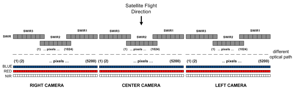
Figure 1.
Instrument configuration schema.
2.2. Radiometric Sensor Model
The Sensor Radiometric Model defines the relationship between the raw digital output as registered by the sensor and the effective spectral radiance at sensor level which is to be derived.
where
k denotes the spectral band,
i is the pixel index,
g is the gain setting, which is a fixed setting per spectral band k,
T is the detector temperature,
DN is the digital number,
(units: LSB(Least Significant Bit)/s) is the dark current coefficient. This coefficient depends on the temperature and the gain setting,
IT is the integration time,
(units: s) is the so-called integration time offset, a parameter introduced allowing the radiometric model fit with calibration results to be improved. This parameter is a fixed setting per spectral band k,
(units: LSB) is the offset per pixel which is dependent on the gain setting,
(units: LSB·W−1·m2·µm·Sr·s–1): is the absolute radiometric coefficient, indicating the sensitivity of the spectral band k,
(unitless) is the equalization coefficient and represents the pixel to pixel light response variation, and is defined for different gain settings. By definition, , the average of over all recorded pixels in a given band k at a given gain setting g, is set to 1.
The values of the different parameters are stored in the radiometric Instrument Calibration Parameters (ICP) files. For each camera, there is a separate ICP file. Initial values for these parameters are given by the on-ground calibration. In-flight updates of the parameters are computed as detailed in the next sections by the PROBA-V Image Quality Center (IQC) and delivered to the User Segment Processing Facility (PF) for the processing of the raw DN images. The level 1C data (i.e., TOA reflectance data in raw geometry) and higher level data contain in their metadata file full traceability to the used ICP file [4]. The TOA reflectance is calculated from the TOA radiance as
with:
: earth-sun distance (astronomical units)
: mean solar exo-atmospheric irradiances for the spectral band k (W/m2/sr)
: solar zenith angle for the spectral band k (degrees)
PROBA-V data users can consult the PROBA-V website (http://proba-v.vgt.vito.be/content/calibration) for an overview of the different updates to the radiometric ICP files.
3. Radiometric Calibration Activities during Commissioning Phase
The commissioning phase lasted for five and half months and was aimed (1) at verification of the platform, the instrument and the complete processing chain and (2) at calibration and validation in order to guarantee that both geometric and radiometric requirements are met before releasing data to the user community. The pre-launch calibration and characterization measurements were used for a first initialization of the different parameters of the sensor radiometric model (1). During the commissioning phase, various vicarious calibration methods were applied, as explained below, to verify these initial parameters independently and to update the calibration parameters in the ICP file.
3.1. Absolute Calibration with the OSCAR Libya-4 Desert Method
Calibration over the Libya-4 desert site relies on a comparison between cloud-free TOA reflectance as measured by PROBA-V and the modelled TOA reflectance values. These modeled values serve as the ‘absolute’ calibration reference and are calculated following [2]. Application of the approach to various satellite data (i.e., AQUA on board MODIS (Moderate Resolution Imaging Spectroradiometer), MERIS (MEdium Resolution Imaging Spectrometer), AATSR (Advanced Along-Track Scanning Radiometer), PARASOL (Polarization & Anisotropy of Reflectances for Atmospheric Sciences coupled with Observations from a Lidar), SPOT-Vegetation) has shown that absolute calibration over the Libya-4 desert is achievable with this approach with an accuracy of 3%. The modelled TOA reflectance values are calculated with the 6SV radiative transfer model using as input : improved Rahman-Pinty-Verstraete (RPV) BRDF model parameters derived from MODIS and MISR data by [2] following the approach originally described in [5], ECMWF meteo data (atmospheric pressure, total column ozone and total column water vapour), a specific desert aerosol model derived for the Sahara region, a monthly variable aerosol optical thickness (AOT) based on an analysis of AERONET and the terrain altitude.
An estimate of the change in the absolute calibration with respect to the on-ground calibration can then be calculated as:
The average result is obtained as:
ith N the number of valid observations.
During the commissioning phase, about 36 scenes from the Libya-4 site were acquired for the LEFT camera, 16 for the CENTER camera and 34 for the RIGHT camera. In Table 1, the average results per band and camera are given.

Table 1.
OSCAR Libya-4 results obtained during commissioning phase.
For the NIR band the PROBA-V Libya4 TOA reflectance values obtained with the pre-flight absolute calibration coefficients were on average 8.3%, 8.6% and 10% higher than the modelled values for the LEFT, CENTER and RIGHT camera, respectively. Considering a maximum possible bias of 3% for the Libya4 desert calibration method [2], it can be concluded that the PROBA-V NIR radiance values, obtained with the pre-flight ICP file, were not within the 5% absolute accuracy requirement and, therefore, an in-flight update of the absolute calibration coefficients for the NIR band was needed for all cameras. For the RED band, the Libya-4 TOA reflectance values obtained with the initial ICP file were on average 4.5%, 3.9% and 6.8% higher than the modelled values for the LEFT, CENTER and RIGHT camera, respectively. Based on the Libya-4 observations, an update of the absolute calibration coefficient for the RED band was needed to achieve a 5% absolute accuracy. For the blue band no significant deviation from one was seen for the LEFT and CENTER camera. For the RIGHT camera is 1.034 (±0.013 stdev) for the observations over Libya4.
The Libya-4 vicarious calibration results were used at the end of commissioning to generate the first in-flight determined absolute calibration parameters (in the following denoted as . For this, a linear regression through the Libya-4 deserts results was performed per camera and per band obtained. Next, the best estimate of was calculated based on the regression coefficients. This approach is preferred to averaging over the period. While the average value would give the best estimate over the whole commissioning phase, it might give an overestimate for the end of commissioning.
3.2. Inter-Band Calibration with the OSCAR Deep Convective Clouds Method
As stated by [6], the benefit of Deep Convective Clouds (DCC) for inter-band calibration compared to bright land targets lies in the fact that DCCs are situated at the top of the atmosphere which minimizes the effect of water vapor and aerosol in the troposphere. Furthermore, Deep Convective Clouds are almost perfect Lambertian scatterers with BRDF effects usually (with the exception of some particular geometrical conditions) smaller than 1% for viewing angles less than 30°. Deep Convective Clouds have a very high TOA reflectance in VNIR wavelengths, with similar spectral shape and with the magnitude of the reflectance in the VNIR mainly determined by the Cloud Optical Thickness (COT). In the red spectral region, the TOA reflectance is reduced due to ozone absorption as the ozone layer is located mainly above the Deep Convective Clouds. After correction for the ozone absorption, the DCC TOA reflectance is almost spectrally white in the 450–900 nm spectral region. According to model simulations performed by [7] Deep Convective Clouds are white (after ozone correction) within 0.5% in the visible, within 1.5% from 670 to 765 nm (excluding oxygen absorption regions) and within 3.5% from 670 to 865 nm. For very dense clouds (with cloud optical depths of 500 or more), a spectral decrease of more than 5% is observed. In the NIR, these deviations are higher than the 3% inter-band accuracy requirement. Therefore, in order to account for these deviations from a perfect white spectral signature, a radiative transfer code is used which allows the TOA spectra to be modelled over Deep Convective Clouds. The RED band is used as a reference band to retrieve the Cloud Optical Thickness (COT) from the measured spectra by comparing against the modelled spectra. The retrieved COT is then used to simulate the TOA reflectance in the other VNIR bands which in turn allows all of the VNIR bands to be compared.
DCC pixels are selected based on a sequence of five tests: (1) a geometry test to reject observations corresponding to viewing geometries near the specular direction; (2) a cloud-land distance test; (3) a NIR reflectance test: a thresholding test is done on the NIR values, as NIR values below the threshold are not strong enough to derive reliable results; (4) a homogeneity test to check if values are sufficiently homogeneous over the samples to derive reliable results and (5) a cloudy neighborhood test to check if the pixel neighborhood is cloudy. If not, the pixel is masked, to avoid influences from non-cloudy pixels. The generation of TOA reflectance Look-Up Tables (LUTs) above Deep Convective Clouds is performed with LibRadtran RTC using the ice particle model from [8]. As cloud reflectance for the VNIR bands is rather insensitive to the effective particle radius, the effective radius is assumed fixed in the DCC calibration process. More details on the LUT generation, image processing (such as pixel selection procedure) and uncertainty analyses can be found in [3].
During the commissioning phase, more than 70 DCC calibration acquisitions, spread over three different ROIs (i.e., Hawaii, Maldives, Pacific East-West), have been performed with the shortest possible integration time (i.e., 0.0012 s) in order to minimize the risk of saturation.
The weighted average inter-band calibration results obtained with the pre-flight absolute calibration coefficients are given in Figure 2a. To calculate the weighted average, the results of the different dates are weighted according to the number of selected pixels in the image after first removing the outlier images based on a 3σ confidence interval from the median. It should be noted that the DCC inter-band calibration is defined with reference to the RED. Results should not therefore be interpreted absolutely, only relatively, indicating the relative differences between bands (inter-band differences). For all cameras, a clear inter-band difference is observed for the pre-flight calibration coefficients. Almost no difference is observed between the different ROIs (figure not shown). Relative to the reference RED band, the radiance in the BLUE band is underestimated by about 2.6%–3.3%. On the other hand, the radiance in the NIR band is, relative to the RED band, overestimated by 3.3%, 2.9% and 1.6% for the LEFT, CENTER and RIGHT camera, respectively. This results in estimated inter-band calibration differences of up to approximately 6.4% for BLUE relative to NIR. These results are consistent with the Libya–4 calibration results obtained with the preflight calibration coefficients, when expressed relative to the RED band.
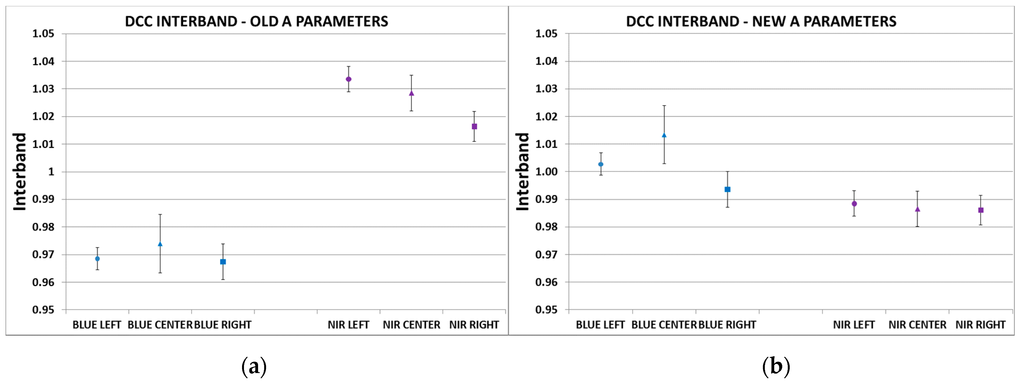
Figure 2.
Inter-band Deep Convective Cloud (DCC) results, relative to the RED reference band: (a) with pre-flight calibration coefficients; (b) with the vicariously updated calibration coefficients (.
A selection of the DCC scenes have been reprocessed using the absolute calibration coefficients determined in-flight. This resulted in a major improvement of the inter-band calibration results (Figure 2b): relative to the RED band both the BLUE and the NIR bands are now well within the 3% inter-band calibration requirement, with relative differences of less than 1.5%. While differences up to 6.5% between BLUE and NIR bands were observed for the initial pre-flight absolute calibration coefficients, BLUE-NIR inter-band differences with the applied are reduced to 1.4%, 2.6% and 0.8% for the LEFT, CENTER and RIGHT camera, respectively.
3.3. Absolute Calibration with the OSCAR Rayleigh Method
Calibration with Rayleigh scattering is performed on pre-defined oligotrophic Rayleigh calibration zones. The primary assumption of the Rayleigh calibration method is that the ocean itself does not contribute to the TOA signal in the NIR for these zones. Under this assumption, the contribution of aerosol scattering (i.e., AOT) can be derived from the NIR reference where molecular scattering is very low assuming a fixed aerosol type. It is assumed here that the NIR reference band is well-calibrated. Once the AOT is determined on the basis of the NIR band, the TOA signal in the other visible bands can be modeled with a radiative transfer code using the appropriate marine reflectance and/or chlorophyll content (CHL). Following [9], the Shettle and Fenn Maritime aerosol model [10] with 98% humidity (denoted as M98) is used. The monthly varying CHL concentration values are taken from [11]. The radiative transfer calculations are done with 6SV. 6SV takes into account the effects of radiation polarization, which is extremely important for radiative transfer calculations over dark targets such as ocean surfaces. As it is computationally prohibitive to run a radiative transfer model for every pixel of all the Rayleigh calibration images, a look-up-table (LUT) approach is used. To reduce the perturbing part of the signal due to ocean reflectance and the presence of foam, strict pixel selection procedures are used as detailed in [3].
The accuracy of the Rayleigh method strongly depends on the accuracy of the radiometric calibration of the reference NIR band. An error in the NIR band directly results in a band-dependent error for the BLUE and RED band Rayleigh Calibration results, due to the high sensitivity of results to the estimated AOT. Analysis of both Libya-4 and DCC results showed clear evidence of excessively high radiance values for the NIR band based on the initial pre-flight calibration coefficients. Results of the Rayleigh calibration for RED and BLUE bands obtained using the initial pre-flight absolute calibration may therefore easily lead to incorrect conclusions (as the Rayleigh method’s basic assumption of a well-calibrated NIR band is violated) and the results are therefore not presented. The results of the Rayleigh calibration, using the vicariously determined A parameters (), are presented in Table 2. These values are well within the required 5% absolute radiometric accuracy.
Table 2.
Absolute Rayleigh calibration results with vicariously updated A coefficients.
3.4. Dark Current
Dark current is caused by thermally generated electrons that build up in the detector’s pixels. Dark current is expected to increase over time due to prolonged exposure to space radiation, and therefore, needs to be regularly monitored. This is done by acquiring data over the nighttime part of the orbit in ocean regions where secondary light sources will be negligible. Acquisitions are done with a long integration time (larger than 200 ms) to increase the radiometric resolution of the result. Monthly averages are calculated for each pixel over all acquisitions and all lines, as well as the standard deviation to get an indication of the reliability of the result. Possible short-term dynamics of the dark signal are evaluated using acquisitions with a short integration time (smaller than 15 ms). At all times, dark current values are rescaled to a reference temperature using the pre-launch sensor model.
The monthly dark current values obtained are compared against monthly values for the previous two months, to assess the stability of the dark current, which can be an indication of defective pixels (see Section 4.3).
4. The Operational Phase
4.1. Camera-to-Camera Bias Adjustments
The calibration updates performed during the commissioning phase ensured that the PROBA-V data delivered to users at the start of the operational phase are within the radiometric calibration requirements. After the commissioning phase, further improvements to the absolute calibration parameters were made in order to correct for a band dependent camera-to-camera bias adjustment. For the camera-to-camera bias assessment, the overlap region between two adjacent cameras is exploited. Since pixels in this zone are seen by the two adjacent cameras under the same sun and view geometry and approximately at the same recording time, BRDF effects have no influence in this calibration and the radiance values of corresponding pixels can therefore be directly compared. The overlap regions of the VNIR cameras contain approximately 75 pixels which is less than 2% of the total number of pixels per VNIR detector strip. A linear regression through the origin is performed for the pairs of overlapping observations and the slope of the regression is calculated. This slope gives an indication of the radiometric difference of the CENTER camera compared to the RIGHT camera and the CENTER camera compared to the LEFT camera, respectively.
This analysis showed minor inter-camera differences for the NIR bands. On the other hand, some inter-camera differences were observed for the BLUE and RED bands, with higher radiance in the CENTER camera overlap regions compared to both the LEFT and RIGHT cameras,
On 26 June 2014, a 1.8% reduction in radiance for the BLUE CENTER strip was applied and a 1.2% increase in radiance of the BLUE RIGHT strip. On 23 September 2014, a reduction of 2.1% was made in the RED CENTER radiance, a 1.1% increase in the BLUE LEFT radiance and a 1.3% increase in the NIR LEFT radiance. Finally, on 25 October 2014, the RIGHT NIR radiance was increased by 1%.
4.2. Stability of the Instrument
The absolute calibration parameters within the ICP files used for Level1c and higher level data processing are corrected for temporal degradation and inter-camera bias (see Section 3.1). For the purpose of the degradation assessment of the instrument response, the results plotted in the temporal drift plots are all generated with a constant absolute calibration parameter () as determined at the end of the commissioning phase.
4.2.1. Trending for the CENTER Camera Based on Lunar Observations
Lunar observations allow the stability of satellites to be monitored thanks to the very high stability of the lunar surface reflectance. Twice a month, PROBA-V acquires lunar images (Figure 3) with a phase angle around 7 degrees before and after full moon. Lunar calibration acquisitions are only obtained with the CENTER camera. The 7° phase angle maximizes the illuminated surface of the moon while avoiding increased uncertainty by minimizing the opposition effect. For each lunar calibration, the radiances observed by PROBA-V are integrated over the lunar image. Although the surface of the moon remains unchanged over the lifetime of PROBA-V, the observed radiance varies due to the moon-observer and moon-sun distances, the difference in phase angles and selenographic angles and variations in the pixel solid angles, and platform rotational speed, also called the oversampling factor.
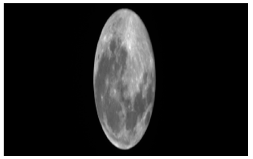
Figure 3.
PROBA-V image of the moon. Due to the oversampling, the along track direction is elongated.
The complexity of these dependencies requires the use of a lunar radiometric model. The USGS lunar calibration program developed such an operational lunar model based on more than 85,000 images acquired by the ground-based Robotic Lunar Observatory (ROLO) [12]. An empirically derived analytical model has fitted all of these ROLO images (which are corrected to TOA radiance, spatially integrated to irradiance, converted to standard distances and finally converted to effective disk reflectance).
The raw lunar images (in DN) are first calibrated to radiometric quantities. Then, the integrated irradiance attributed to the moon is determined by summing all pixels on the lunar disk including the unlit portion. A critical aspect here is the determination of the lunar disk, which might be rather subjective. Different techniques are published in the literature. In [13], a threshold technique, combined with a proximity test, is used to select the on-moon pixels. In the automated processing of the PROBA-V lunar calibration images, a similar technique is used.
In Figure 4, the PROBA-V lunar calibration results normalized to the first observation are given for the BLUE, RED, NIR and SWIR2 strips of the center camera. A linear regression is fitted to the data to quantify degradation over time:
where t is the number of days since launch. The slope of the linear regression is given by:
with n the number of lunar calibration results per band.
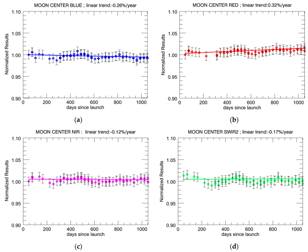
Figure 4.
Normalized PROBA-V lunar calibration results depicted with 3% error bars: (a) CENTER BLUE strip; (b) CENTER RED strip; (c) CENTER NIR strip and (d) CENTER SWIR1 strip. Bold lines: fitted linear regression model.
The slope of this regression line is very small: a very minor negative trend is observed for the BLUE, NIR and SWIR2 strips with −0.26%/year, –0.12%/year and −0.17%/year, respectively. For the RED band, a slight positive trend of 0.32%/year is visible.
Slight seasonal trends are observed in the lunar calibration results. These are mainly related to inaccuracies in estimating disc irradiance or disc equivalent reflectance. To define the total irradiance from the image, all of the pixels in the image need to be detected correctly and the so- called solid angle derived. Errors in the selection of the moon pixels and, consequently, in the derivation of the solid angle are typical causes for seasonal trends. The SWIR band has the largest uncertainty in the selection of the moon pixels, due to the lower resolution (less pixels). This translates into a larger diurnal variation compared to the VNIR. An investigation is currently under way to determine whether other techniques, such as canny edge detection, are better suited.
4.2.2. Trending for All Cameras Based on Libya-4 Observations
The OSCAR Libya-4 desert approach has been applied to all cloud-free PROBA-V observations performed over this desert site and the trend over time is analyzed. It is important to repeat that, for these analyses, a constant absolute calibration has been used in order to capture the actual degradation of the instrument response over time. Despite the application of a BRDF model, a seasonal trend has been observed in the results for all cameras and strips (illustrated in Figure 5a and Figure 6a for the center RED and NIR strip). The magnitude and phase of the seasonal oscillation can be fairly well modelled with a simple cosine function (see black circles in Figure 5 and Figure 6). This cosine function is used to correct the individual results for the seasonal trend as depicted in Figure 5b and Figure 6b. The degradation since launch is then calculated by fitting a linear regression model to the corrected data.
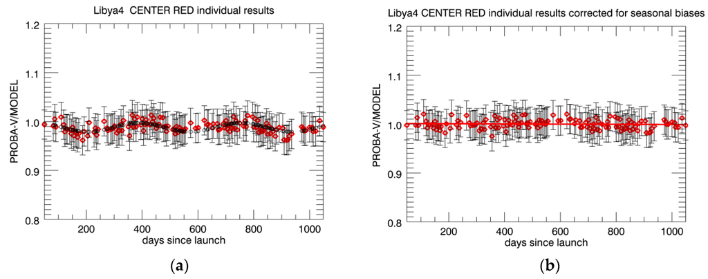
Figure 5.
OSCAR Libya-4 PROBA-V results: (a) red diamonds: individual CENTER RED strip results (obtained using a constant absolute calibration parameter) depicted with 3% error bars; Black circles: fitted cosine function; (b) OSCAR Libya-4 results corrected for seasonal trend and fitted linear model.
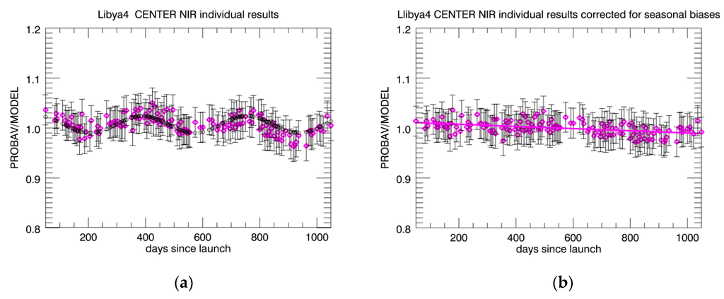
Figure 6.
Same as Figure 5, but for CENTER NIR strip. (a) magenta diamonds: individual CENTER NIR strip results (obtained using a constant absolute calibration parameter) depicted with 3% error bars; Black circles: fitted cosine function; (b) OSCAR Libya-4 results corrected for seasonal trend and fitted linear model.
In Table 3, the linear trend per year obtained under this approach is given for the different strips and cameras. The table includes also the linear trend as obtained with the lunar calibration approach. For all VNIR strips, the observed degradation is less than 1%/year, with negligible trends observed for the RED strips (between −0.08%/year and −0.24%/year) and the largest one for the NIR strips (between −0.58%/year and −0.85%/year). The Libya-4 results therefore confirm the good stability of the VNIR strips as also observed in the lunar calibration results. Some more significant degradation trends, between −1.25%/year and −1.96%/year depending on the strip, are observed for the SWIR strips. This slight degradation trend was not clearly noticeable in the lunar results. This might be due to the higher uncertainty in SWIR lunar calibration results, caused by the difficulty in delineating the on-Moon pixels correctly and consistently over time.
Table 3.
Linear trend per year as calculated over the seasonal corrected OSCAR Libya-4 PROBA-V results and the Moon calibration results, both obtained with a constant absolute calibration.
4.3. Dark Current Evolution
The evolution of dark current over time will show an increase which is expected to be linear over time, assuming a roughly constant radiation dose [14,15]. Also, high similarities are expected to be found for the majority of pixels in the instrument, as these will have experienced similar levels of radiation. Some trends of difference exist between (1) VNIR and SWIR sensors; (2) different bands of the VNIR sensor; (3) different cameras. These will be reviewed by looking at the evolution of average dark current in a detector line, in Section 4.3.1. Apart from these trends, individual pixels can behave as outliers and behave differently from the average pixels in a detector line. These outliers are reviewed in Section 4.3.2.
4.3.1. Average Dark Current Evolution
For the VNIR sensors, dark current values for all pixels are negligible, considering also the low integration times used during nominal operations (maximum 6 ms). In Figure 7, the average dark current evolution for each VNIR band is shown, from the start of the operational phase up to 19 April 2016. The dark current values are rescaled to the reference temperature of −10 °C, according to the pre-launch dark current temperature relationship. The increase in dark current shows a consistent linear relationship for each band, excluding small variations at the start of the operational phase, between October and November 2013. Linear regression functions for each band are provided in Table 4, together with a predicted dark current value at the end of the operational lifetime (end-of-life, or EOL). Even at EOL, the dark current for all VNIR bands is barely noticeable. Comparing cameras for the same bands, the same dark current levels are found and this applies for all bands. Differences are found in the dark current of different bands. This is explained by the different gain settings in the Analog-to-Digital Converter, which scales the analog dark current to a different digital level. The difference in dark current is explained fully by this difference in scale (5.8 V/V for Blue compared to 2.29 V/V for Red and 1.99 V/V for NIR).
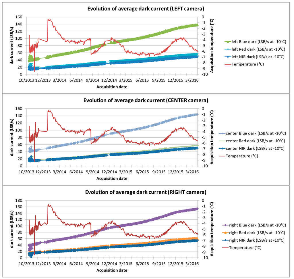
Figure 7.
Evolution of average dark current for PROBA-V VNIR bands (15 October 2013 to 19 April 2016).
Table 4.
Regression and End-of-Life estimation of dark current for the PROBA-V VNIR bands at a reference temperature of −10 °C and for an IT of 0.006 s.
For the SWIR sensors, the average dark current level is also quite low but slightly higher than for the VNIR sensors, considering the higher integration times used in nominal operations (maximum 24 ms). Figure 8 shows the average dark current evolution for each SWIR band, from the start of the operational phase up to 19 April 2016, and with values rescaled to the reference temperature of −10 °C. A slight drop of about 2LSB/s in the linear trend is noticed after 16 January 2015, which coincides with the decision to adopt a lower integration time for SWIR dark calibration acquisitions (0.2048 s instead of 2.9696 s). As this effect is minor, results for linear regression are provided for the full evaluation period (Table 5). The predicted EOL average dark current levels are still sufficiently low as to not impede the operational mission. Differences are observed between cameras (the right camera sensors show a higher rate of increasing dark current) and between individual sensors (all SWIR2 or ‘middle’ sensors show a higher dark current than their counterparts SWIR1 and SWIR3).
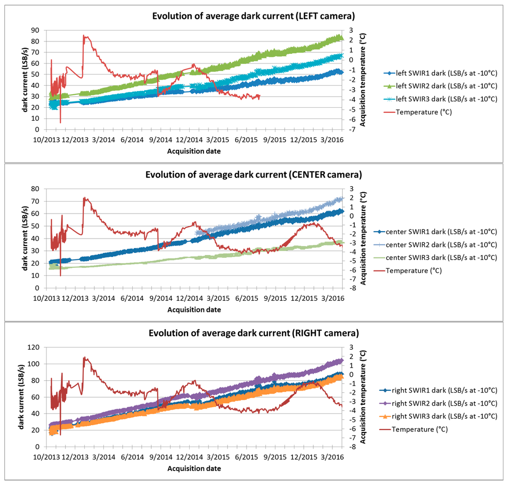
Figure 8.
Evolution of average dark current for PROBA-V SWIR bands (15 October 2013 to 1 April 2016).
Table 5.
Regression and End-of-Life (EOL) estimation of dark current for PROBA-V SWIR bands at a reference temperature of −10 °C and for an IT of 0.020 s (L = Left, C = Center, R = Right).
4.3.2. SWIR Dark Current Outliers
Even in commissioning, some SWIR pixels showed a considerably higher dark current than the average dark current on the SWIR sensors. When the dark current exceeds 200 LSB/s at −10 °C, but is stable and does not impede the dynamic range of the sensor, such pixels are classified as ‘good but with high dark current’ (labeled “H DC OK”). However, some pixels also show unstable dark current levels, changing over time, and making calibration difficult and the pixel values unreliable. If differences between monthly averages of more than 200 LSB/s exist at a reference temperature of −10 °C, the pixels are initially classified as ‘suspicious and with high dark current’ (labeled ‘H DC NOK’). The threshold of 200LSB/s at −10 °C is quite low for all nominal integration times (less than 5 LSB at −10 °C for the maximum integration time of 24 ms), implying that all “H DC OK” pixels can be considered sufficiently stable to allow good calibration. The “H DC NOK” pixels are further analyzed by image quality experts to assess whether the response to nominal light conditions is also impacted. Pixels with otherwise unusual behavior in light conditions are also analyzed. If it is concluded that light response is also impacted, the pixel is assigned a “BAD” quality state in the ICP files. A list of all “BAD” pixels thus analyzed is provided in Table 6, showing the status as of March 2016. This amounts to 0.3% of all valid pixels (less than 10 pixels per sensor). The values of these pixels is interpolated in the PROBA-V End-User products, and the quality of the pixels can be retrieved from the status map layer.
Table 6.
List of SWIR pixels classified as “BAD” on PROBA-V (Status on Mid-March 2016).
In a similar way to the average dark current, there has been a steady increase in pixels detected as “H DC OK”, or a dark current higher than 200 LSB/s at −10 °C. This corresponds to 4.8 LSB for an integration time of 24 ms, indicating that even these pixels should not impede the dynamic range of the sensor. To put these results in perspective, the number of pixels exceeding 40 LSB for an integration time of 24 ms has also been reported in the most recent measurements on February 2016.
The number of pixels classified as “H DC OK” is shown in Figure 9 in function of time. By end of the mission, 23.59% of all pixels are expected to be classified as “H DC OK”, with 14.28% already classified on 1 March 2016. However, only 0.9% of all pixels on 1 March 2016 has a dark current exceeding 40 LSB at 24 ms integration time (Table 7). This also includes pixels which have been classified as “H DC BAD”.
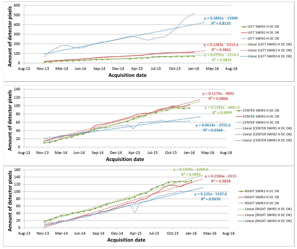
Figure 9.
Evolution of number of pixels classified as “High dark current and good” (HDC OK) for PROBA-V SWIR bands (December 2013 up to February 2016).
Table 7.
Regression parameters and End-of-Life (EOL) estimate of High Dark Current (HDC) for PROBA-V SWIR bands (L = Left, C = Center, R = Right).
The Left SWIR3 sensor shows a considerable number of pixels classified as “H DC”, and a marked increase of such pixels since October 2015. This will be monitored closely and adequate action will be taken if the quality of the measurements is impacted because of the dark current evolution.
5. Independent Validation
The radiometric monitoring of the PROBA-V instrument is also carried out independently from the Image Quality Center (IQC) activities through the so-called DIMITRI (Database for Imaging Multi-spectral Instruments and Tools for Radiometric Intercomparison) tool available at the European Space Research and Technology Centre (ESTEC) and adapted to PROBA-V for the commissioning phase of the mission. The radiometric monitoring of the instrument is based on the comparison of (a) the TOA reflectance from the operational PROBA-V L1C products (i.e., TOA reflectance in raw geometry) averaged over the Libya-4 site and (b) TOA reflectance simulated following the methodology for pseudo-invariant desert calibration sites described in [16].
Two types of simulated TOA reflectances are generated for comparison to the operational PROBA-V L1C products:
- Simulated in-band PROBA-V TOA reflectance resulting from the convolution of simulated hyperspectral TOA reflectance and the PROBA-V VNIR channels spectral response functions. The simulated hyperspectral TOA reflectance over Libya-4 simulations are the output of a coupled surface atmosphere Monte Carlo radiative transfer model fully describing both absorption and scattering events [16]. The surface BRDF model parameters used as input to the radiative transfer model were derived from the inversion of the BRDF surface parameters enabling the TOA model simulations to best mimic four years (2006–2009) of MERIS TOA observations over the site.
- Simulated in-band VGT-2 TOA reflectance. The simulation of the VGT-2 is done following the same approach described in [16] but by substituting the surface BRDF model parameters derived from MERIS TOA observations with BRDF surface parameters, enabling the best mimicking of four years (2006–2009) of VGT-2 TOA observations over the site. Such VGT-2 top-of-atmosphere reflectance are not directly comparable to the PROBA-V observation as the spectral response of these two instruments differs noticeably. This comparison is however useful for Proba-V users that are also VGT-2 historical data users in order to provide estimates of the radiometric (dis)continuity that might exist between the two instrument measurement time series. These differences between PROBA-V and VGT-2 measurements are expected to be a combination of differences both in radiometric calibration and in spectral response functions.
Time series of the relative difference between the PROBA-V TOA reflectance and the simulated PROBA-V TOA reflectance are illustrated in Figure 10. A synthesis of the statistical analysis of the time series obtained for each TMA (Three-Mirror Anastigmatic) telescope and spectral band is presented in Table 8. The comparison is restricted to the VNIR channels because the MERIS spectral coverage only allows the retrieving of surface BRDF model parameters in the 400–900 nm spectral range.
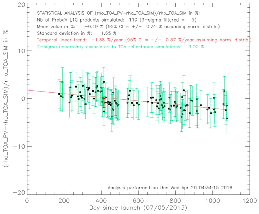
Figure 10.
Time series of relative difference in % between the PROBA-V TOA reflectance in the BLUE band of the CENTER TMA and the simulated PROBA-V reflectance using a hyperspectral TOA model with BRDF surface parameters inverted from four years of MERIS TOA data. The statistical analysis of the time series provides the mean relative difference, the standard deviation and the temporal trend obtained from a linear fitting of the time series. A 95% confidence interval on the mean relative difference and the temporal trend is obtained assuming a normal distribution of the mean relative difference. The green error bar represent the uncertainty associated to each simulation of the PROBA-V TOA reflectance. The red bar located around day 400 since launch indicates the change (decrease) in radiometric calibration applied to the PROBA-V L1C processing.
Table 8.
Synthesis of the statistical analysis of the time series of relative differences between the PROBA-V TOA reflectance values and their simulation.
Time series of the relative difference between the PROBA-V TOA reflectance and the simulated VGT-2 TOA reflectance are illustrated in Figure 11. A synthesis of the statistical analysis of the time series obtained for each TMA and spectral band is presented in Table 9.
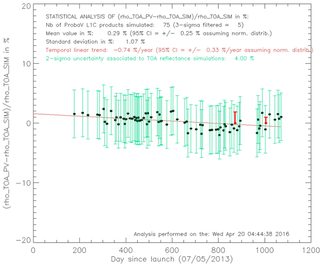
Figure 11.
Time series of the relative difference in % between the PROBA-V TOA reflectance in the SWIR2 band of the LEFT TMA and the simulated PROBA-V reflectance using a hyperspectral TOA model with BRDF surface parameters inverted from four years of MERIS TOA data. The statistical analysis of the time series provides the mean relative difference, the standard deviation and the temporal trend obtained from a linear fitting of the time series. A 95% confidence interval on the mean relative difference and the temporal trend are obtained assuming a normal distribution of the mean relative difference. The green error bar represent the uncertainty associated to each simulation of the PROBA-V TOA reflectance. The red bars located around day 850 and 1000 since launch represent the change (increase) in radiometric calibration applied to the PROBA-V L1C processing.
Table 9.
Synthesis of the statistical analysis of the time series of the relative difference between PROBA-V TOA reflectance and the simulation of VGT-2 TOA reflectance.
A good consistency is found between PROBA-V and MERIS TOA reflectance data (Table 8). PROBA-V TOA reflectance values appear to be slightly lower than the MERIS TOA reflectance values, by 0.5%–2.5% depending on the band. The slight temporal trend observed in the blue (Figure 10, Table 8) and the red (Table 8) band of the CENTER camera are partly due to inter-camera bias adjustments (see Section 3.1) performed on 26 June 2014 and 23 September 2014, respectively. No reprocessing of the L1C data acquired before these dates has yet been done. The reprocessing is expected to be done in the second quarter of 2016. Except for these bands, observed temporal trends in the L1C VNIR data are very small, i.e., within +0.05%/year and −0.37%/year. These trends are not statistically significant at a 95% confidence level.
Whereas the MERIS PROBA-V VNIR TOA reflectance values are slightly lower than the MERIS values, they are a between 0.76% and 4.49% higher than the VGT2 values (Table 9). This is explained mainly by the fact that for RED and NIR bands in particular there is a negative bias of about 4% between VGT2 and MERIS, as documented by various authors [2,16,17,18]. For the BLUE band, the largest difference with respect to VGT-2 is observed for the PROBA-V CENTER camera and clear differences exist between the cameras. This might be partly due the known smile pattern (View Zenith Angle (VZA) dependency of the TOA reflectance values) in the VGT-2 blue data [3,16].
For the SWIR, a good agreement is observed between the PROBA-V and VGT-2 with differences of less than 1% (Table 9, Figure 11), except for the SWIR 3 strip of the RIGHT camera. Observed temporal trends are relatively small, between 0.66%/year and −0.92%/year, and significantly less than the observed degradation in the instrument response as reported in Section 3.2 This is mainly due to the different SWIR absolute calibration parameter updates in the ICP files, used for generating the L1C data, in order to correct for the observed degradation in the SWIR bands.
6. Conclusions and Outlook
On-orbit radiometric performance is continuously monitored and calibration parameter updates are regularly performed to ensure that the radiometric accuracy requirements are met. Both lunar and Libya-4 observations show that instrument response degradation is small for all the VNIR strips with changes in responsivity well below 1% per year. A slightly larger degradation is observed over Libya-4 for the SWIR strips. The radiometric values of the PROBA-V L1C VNIR data appear to be situated between the MERIS radiometric values and SPOT VGT-2 ones.
As all vicarious validation methods have their own limitations and uncertainties, in-flight calibration that has to rely solely on vicarious methods is a challenging process. Uncertainty in the vicarious calibration results arises from, among other things, the assumptions underlying the methods, the intrinsic uncertainty of the radiative transfer and/or BRDF models used and errors in ancillary input data (such as meteo and aerosol data). By applying a set of different vicarious calibration methods and comparing the respective results, systematic errors inherent to one or more of the methods are reduced. Due to the relatively large random error associated with a single vicarious calibration result, statistical averaging over several observations is needed to deal with these random errors. Furthermore, some methods such as the OSCAR calibration over the Libya-4 deserts site seem to be prone to season-dependent biases. Due to the uncertainties in the results, frequent absolute calibration updates based on individual results would lead to fluctuations. It takes some time before sufficient vicarious observations are acquired to distinguish an instrument related degradation trend from ‘noise’. This is further complicated by the fact that the different strips within and between the three PROBA-V cameras may show varying degradation patterns (note that there are nine SWIR strips, which may vary in stability) and the lack of a pre-flight determined degradation model. Consequently, updating the absolute calibration coefficients is not a smooth and gradual adjustment, but instead a more step-wise adjustment process (see for example Figure 11) based on the significance of the observed trend. To improve the smoothness of the absolute calibration parameter updates, a linear trending model has now been fitted to vicarious calibration results collected over more than 2.5 years. This function will be used to predict the absolute calibration parameter valid for the next month based on all previously acquired data, without risk of unwanted fluctuations in the updates. Additionally, a trending model enables smooth calculation of the changes in absolute calibration parameters over the previous months, and these will be used for the first reprocessing of the PROBA-V archive. The reprocessing is planned for the second quarter of 2016, and will also include correction of the inter-camera bias adjustment from the start of the mission and an improved cloud detection algorithm.
The distribution of the cameras with butted SWIR detectors and the lack of on-board diffusers for flat-fielding purposes makes in-flight correction for non-uniformities a challenging issue. In order to better characterize and correct for non-uniformities within and between detectors, a 90° yaw maneuver has recently (i.e., on 11 April 2016) been performed with PROBA-V over the Niger-1 desert site. With this 90° yaw configuration, the detector array runs parallel to the direction of the motion and, therefore, a given area on the ground is subsequently viewed by the different pixels of the same spectral band. Due to the butted design of the SWIR detectors, six of the nine SWIR strips will observe the same area, while the other three SWIR strips will observe a different area. The data are currently being processed with the aim of correcting for residual non-uniformities in the data.
Acknowledgments
The authors wish to thank Tom Stone (USGS) for fruitful discussions on the ROLO model and Yves Govaerts (Rayference) for his valuable input during the commissioning phase. The authors furthermore acknowledge the contribution of teams from Qinetiq Space, OIP, ESA and Spacebel. This work was supported by Belspo (contract CB/67/8) and ESA (contract 091669 and 4000111291/14/I-LG).
Author Contributions
Sindy Sterckx leads the radiometric Image Quality Center for the PROBA-V mission and wrote the first draft of the paper with the help from all authors. Stefan Adriaensen implemented the different calibration algorithms in automated workflows and performed the lunar calibration analyses. Wouter Dierckx is the PI of PROBA-V and provided the analyses for the dark current. Marc Bouvet performed the inter-comparison against MERIS and VGT-2.
Conflicts of Interest
The authors declare no conflict of interest
References
- Dierckx, W.; Sterckx, S.; Benhadj, I.; Livens, S.; Duhoux, G.; Van Achteren, T.; Francois, M.; Mellab, K.; Saint, G. PROBA-V mission for global vegetation monitoring: Standard products and image quality. Int. J. Remote Sens. 2014, 35, 2589–2614. [Google Scholar] [CrossRef]
- Govaerts, Y.; Sterckx, S.; Adriaensen, S. Use of simulated reflectances over bright desert target as an absolute calibration reference. Remote Sens. Lett. 2013, 4, 523–531. [Google Scholar] [CrossRef]
- Sterckx, S.; Adriaensen, S.; Livens, L. Rayleigh, Deep convective clouds and cross sensor desert vicarious calibration validation for the PROBA-V mission. IEEE Trans. Geosci. Remote Sens. 2013, 51, 1437–1452. [Google Scholar] [CrossRef]
- Sterckx, S.; Benhadj, I.; Duhoux, G.; Livens, S.; Dierckx, W.; Goor, E.; Adriaensen, S.; Heyns, W.; Van Hoof, K.; Strackx, G.; et al. The PROBA-V mission: Image processing and calibration. Int. J. Remote Sens. 2014, 35, 2565–2588. [Google Scholar] [CrossRef]
- Govaerts, Y.M.; Clerici, M. Evaluation of radiative transfer simulations over bright desert calibration sites. IEEE Trans. Geosci. Remote Sens. 2004, 42, 176–187. [Google Scholar] [CrossRef]
- Chen, L.; Hu, X.; Xu, N.; Zhang, P. The application of deep convective clouds in the calibration and response monitoring of the reflective solar bands of fy-3a/mersi (medium resolution spectral imager). Remote Sens. 2013, 5, 6958–6975. [Google Scholar] [CrossRef]
- Fougnie, B.; Bach, R. Monitoring of radiometric sensitivity changes of space sensors using deep convective clouds: Operational application to PARASOL. IEEE Trans. Geosci. Remote Sens. 2009, 47, 851–861. [Google Scholar] [CrossRef]
- Baum, B.A.; Yang, P.; Heymsfield, A.J.; Platnick, S.; King, M.D.; Hu, Y.X.; Bedka, S.M. Bulk scattering models for the remote sensing of ice clouds: Part 2: Narrowband models. J. Appl. Meteorol. 2005, 44, 1896–1911. [Google Scholar] [CrossRef]
- Hagolle, O.; Goloub, P.; Deschamps, P.-Y.; Cosnefroy, H.; Briottet, X.; Bailleul, T.; Nicolas, J.-M.; Parol, F.; Lafrance, B.; Herman, M. Results of polder in-flight calibration. IEEE Trans. Geosci. Remote Sens. 1999, 37, 1550–1566. [Google Scholar] [CrossRef]
- Shettle, E.; Fenn, R.W. Models for the Aerosols of the Lower Atmosphere and the Effects of Humidity Variations on their Optical Properties; Environment. Research. Paper. No. 676; AFGL-AFSC: Hanscom AFB, MA, USA, 1979. [Google Scholar]
- Morel, A.; Claustre, H.; Gentili, B. The most oligotrophic subtropical zones of the global ocean: similarities and differences in terms of chlorophyll and yellow substance. Biogeosci. Discuss. 2010, 7, 5047–5079. [Google Scholar] [CrossRef]
- Kieffer, H.; Stone, T.C. The spectral irradiance of the Moon. Astron. J. 2005, 129, 2887–2901. [Google Scholar] [CrossRef]
- Stone, T.C.; Rossow, W.B.; Ferrier, J.; Finkelman, L.M. Evaluation of ISCCP multisatellite radiance calibration for geostationary imager visible channels using the Moon. IEEE Trans. Geosci. Remote Sens. 2013, 51, 1255–1266. [Google Scholar] [CrossRef]
- Bentell, J.; Van der Zanden, K.; Colin, T.; Herftijd, S.; Merken, P.; Vermeiren, J.A. Comparitive study of the MSI and Proba-V linear arrays under the influence of radiation. In Proceedings of the Fourth International Workshop on Analogue and Mixed Signal Integrated Circuits for Space Applications (AMICSA), Noordwijk, The Netherlands, 26–28 August 2012.
- Hopkinson, G.R. Radiation-induced dark current increases in CCDs. In Proceedings of the Second European Conference on Radiation and its Effects on Components and Systems (RADECS), St. Malo, France, 13–16 September 1993; pp. 401–408.
- Bouvet, M. Radiometric comparison of multispectral imagers over a pseudo-invariant calibration site using a reference radiometric model. Remote Sens. Environ. 2014, 140, 141–154. [Google Scholar]
- Adriaensen, S.; Barker, K.; Bourg, L.; Bouvet, M.; Fougnie, B.; Govaerts, Y.; Henry, P.; Kent, C.; Smith, D.; Sterckx, S. CEOS Ivos Working Group 4: Intercomparison of Vicarious Calibration and Radiometric Intercomparison over Pseudo-Invariant Calibration Sites. 2012. Available online: http://calvalportal.ceos.org/ceos-wgcv/ivos/wg4/final-report (accessed on 20 June 2016).
- Lachérade, S.; Fougnie, B.; Henry, P.; Gamet, P. Cross Calibration over Desert Sites: Description, Methodology, and Operational Implementation. IEEE Trans. Geosci. Remote Sens. 2013, 51, 1098–1113. [Google Scholar] [CrossRef]
© 2016 by the authors; licensee MDPI, Basel, Switzerland. This article is an open access article distributed under the terms and conditions of the Creative Commons Attribution (CC-BY) license (http://creativecommons.org/licenses/by/4.0/).