Abstract
Regional haze episodes have occurred frequently in eastern China over the past decades. As a critical indicator to evaluate air quality, the mass concentration of ambient fine particulate matters smaller than 2.5 μm in aerodynamic diameter (PM2.5) is involved in many studies. To overcome the limitations of ground measurements on PM2.5 concentration, which is featured in disperse representation and coarse coverage, many statistical models were developed to depict the relationship between ground-level PM2.5 and satellite-derived aerosol optical depth (AOD). However, the current satellite-derived AOD products and statistical models on PM2.5–AOD are insufficient to investigate PM2.5 characteristics at the urban scale, in that spatial resolution is crucial to identify the relationship between PM2.5 and anthropogenic activities. This paper presents a geographically and temporally weighted regression (GTWR) model to generate ground-level PM2.5 concentrations from satellite-derived 500 m AOD. The GTWR model incorporates the SARA (simplified high resolution MODIS aerosol retrieval algorithm) AOD product with meteorological variables, including planetary boundary layer height (PBLH), relative humidity (RH), wind speed (WS), and temperature (TEMP) extracted from WRF (weather research and forecasting) assimilation to depict the spatio-temporal dynamics in the PM2.5–AOD relationship. The estimated ground-level PM2.5 concentration has 500 m resolution at the MODIS satellite’s overpass moments twice a day, which can be used for air quality monitoring and haze tracking at the urban and regional scale. To test the performance of the GTWR model, a case study was carried out in a region covering the adjacent parts of Jiangsu, Shandong, Henan, and Anhui provinces in central China. A cross validation was done to evaluate the performance of the GTWR model. Compared with OLS, GWR, and TWR models, the GTWR model obtained the highest value of coefficient of determination (R2) and the lowest values of mean absolute difference (MAD), root mean square error (RMSE), and mean absolute percentage error (MAPE).
1. Introduction
Epidemiologic studies demonstrated that fine particulate matters smaller than 2.5 μm in aerodynamic diameter (PM2.5), associated with increased cardiopulmonary and cardiovascular mortality, have a significant negative impact on human health [1,2,3,4,5]. The measurement of pollutant concentrations including ground-level PM2.5 is therefore performed regularly in many industrialized countries that have established air quality monitoring stations a short distance from residential or manufacturing districts [6,7,8,9]. Traditional air quality estimations from ground-based stationary ambient measurements, though deemed to be accurate and precise, are insufficient in that the coarse spatial coverage and irregular distribution of monitoring networks largely restrict the environmental studies to ground-level PM2.5 concentration, which demand spatial-temporal dynamics of air pollutants in high resolution [10,11].
In contrast to traditional ground measurements, satellite remote sensing can offer a more effective means of monitoring and estimating the concentration of atmospheric contaminants and their variation on a synoptic map over large area. To provide atmospheric parameter estimations with extensive spatial coverage for air pollution studies, satellite remote sensing of ground-level PM2.5 concentration is becoming increasingly important. Previous studies have demonstrated that ground-level PM2.5 concentrations in a large area can be estimated from satellite-derived aerosol optical depth (AOD) referring to other supplemental factors [12]. AOD is a measure of columnar light extinction by aerosol scattering and absorption during the satellite overpass and is related to the loading of fine particulate matters in the column [13]. Currently, AOD products from many satellite sensors such as the Moderate Resolution Imaging Spectroradiometer (MODIS) with 10 km × 10 km spatial revolution [14,15,16], the Multiangle Imaging SpectroRadiometer (MISR) with 17.6 km × 17.6 km spatial revolution [17,18,19], and the Geostationary Operational Environmental Satellite Aerosol/Smoke Product (GASP) with 4 km × 4 km spatial revolution [20,21,22] have been used to provide globally estimation of ground-level PM2.5 concentrations. However, the coarse spatial resolution of the aforementioned AOD products is insufficient for air environmental monitoring and haze tracking at the urban or regional scale, which demand finer spatial revolution of ground-level PM2.5 concentrations.
Remarkable progress has been achieved in establishing the quantitative relationship between satellite-derived AOD and ground-level PM2.5 concentrations. Without considering the spatial and temporal variations in the PM2.5–AOD relationship, a linear regression model [23,24,25] was firstly introduced to estimate ground-level PM2.5 concentrations. Furthermore, meteorological variables were incorporated into the PM2.5–AOD model to improve the estimation accuracy. For instance, Tian and Chen [26] proposed a semi-empirical model applying the assimilated planetary boundary layer height (PBLH) corrected and ambient meteorological conditions adjusted MODIS AOD to estimate the hourly concentration of ground-level PM2.5 coincident to a satellite overpass at a regional scale. Subsequently, a number of empirical models were developed, including the linear or nonlinear regression model [11,27,28,29] and artificial neural network (ANN) model [30,31]. However, the performance of the above models becomes poorer when the modeling domain gets larger.
To assess the potentiality of GOES aerosol/smoke product (GASP) AOD acting as a proxy for ground-level PM2.5 in the United States, Paciorek et al. [32] analyzed the strength of association between AOD and ground-level PM2.5 based on daily, monthly, and yearly averages, and found low daily correlations in the PM2.5–AOD relationship over time at fixed locations during the winter or over space at fixed times. That is to say, drastic variability in the PM2.5–AOD relationship was displayed in different regions at different time scales, and the PM2.5–AOD correlation is not constant across space or time, but changes with spatial and temporal contexts. In order to estimate location-specific ground-level PM2.5 concentration, a novel linear mixed effects model allowing temporal variability in daily PM2.5–AOD relationships was constructed by Lee et al. [33]. The common land use regression (LUR) variables and meteorological factors were then employed to extend the linear mixed effects model to provide spatio-temporally resolved ground PM2.5 estimations of short term and long-term human exposures [11]. However, these models still conceptually disregarded the spatial and temporal variability and non-stationarity of PM2.5–AOD relationships that might bring significant biases into PM2.5 estimation. Hu et al. [34] presented a geographically weighted regression (GWR) model to examine the relationship among ground-level PM2.5 concentrations, satellite-derived AOD, meteorological variables (either ground-observed or assimilation), and land use dataset, and then established a two-stage AOD–PM2.5 estimation algorithm [13]. Referring to satellite overpassing over the Pearl River Delta region in China, Song et al. [35] applied a GWR model to estimate the daily concentration of ground-level PM2.5 with MODIS AOD. Focusing on large-scale spatial and temporal variability comparison between satellite-derived AOD and PM2.5, Li et al. [36] found diverse, even opposite, seasonal cycles in the PM2.5–AOD relationship owing to the varied height of the atmospheric mixing layer. Such studies highlighted the importance of spatio-temporal variability in PM2.5–AOD relations, but failed to explicitly and simultaneously incorporate variable factors into models to infer ground-level PM2.5 concentrations from satellite AOD estimations. Referring to the shortage of ground-level PM2.5 concentration of high spatio-temporal revolution for air quality monitoring and population exposure studies, we aim to develop a flexible estimation model to calibrate the satellite-derived AOD at 500 m spatial revolution to hourly ground-level PM2.5 concentrations.
In this article, a geographically and temporally weighted regression (GTWR) model based on a satellite-derived AOD is proposed to estimate hourly ground-level PM2.5 concentration images with fine spatial resolution at the regional scale. First, a simplified high-resolution MODIS aerosol retrieval algorithm (SARA) is selected to produce satellite-derived AOD images with 500 m spatial resolution. Second, the weather research and forecasting (WRF) model is employed to extract the hourly meteorological field data. Third, we examine and compare the quality of PM2.5 estimations from GTWR to ordinary least squares (OLS), GWR, and temporally weighted regression (TWR) methods by means of case study. The case study region, named JSHA linking region, is a famous fossil energy base that covers the adjacent parts of Jiangsu, Shandong, Henan, and Anhui provinces in central China.
2. Materials and Methodology
2.1. Study Region
With rapid economic development and urbanization, the consumption of fossil fuels including coal and petroleum has increased dramatically in China, resulting in severe regional air pollution and frequent haze episodes. The JSHA linking region takes Xuzhou as its center, which extends about 150 km to the north, west, and south from Xuzhou, and about 50 km to the east from Xuzhou (see Figure 1). The study region includes a large number of coal mines and thermal power plants, and numerous cities with a population of hundred thousands to several million. This particular economic region suffers frequently from haze episodes, especially in the winter heating period, due to coal burning in heating stations and power plants.
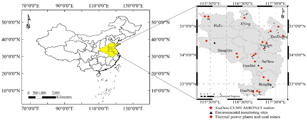
Figure 1.
Location of AERONET station and environmental monitoring stations in the JSHA study region.
2.2. Data
2.2.1. Satellite-Derived AOD
With the evolution of satellite remote sensing sensors and retrieval algorithms, more and more satellite-derived AOD products have been employed to estimate the ground-level PM2.5 concentration. The MODIS AOD product with high temporal resolution has been widely used, twice a day, for environmental monitoring in numerous studies. However, its coarse spatial resolution of 10 km × 10 km does not allow detailed regional- or urban-scale air quality monitoring. In this article, the SARA algorithm developed by Bilal et al. [37], which shows higher accuracy and better reliability in AOD retrieval than the MODIS 04 algorithm over the complex surfaces under low and high aerosol loadings with mixed aerosol types [38], is used to generate high-resolution MODIS AOD images. SARA is applied with the Radiative Transfer Model (RTM) to directly calculate MODIS AOD at 500 m resolution based on MODIS (Terra/AQUA) level 1 (MOD02HKM calibrated radiance and MOD03 geolocation data) and level 2 (MOD09 surface reflectance) products with aerosol properties including single scattering albedo (SSA) and asymmetry parameter obtained from the Aerosol Robotic Network (AERONET) station at China University of Mining and Technology (http://aeronet.gsfc.nasa.gov/). The temporal averaging on the AERONET product is done within ±30 min of the MODIS local overpass moment.
2.2.2. Ground-Level PM2.5 Measurements
For the sake of monitoring and supervising the air quality in China, the Ministry of Environmental Protection of the People Republic of China has established more than 1497 monitoring stations over 367 cities and collects the measurements of PM10, PM2.5, SO2, NO2, O3, and CO in real time. In this study, hourly averaged PM2.5 concentrations when the satellite passes over the study region were downloaded from the national air quality publishing platform (http://106.37.208.233:20035/). The locations of Xuzhou-CUMT AERONET station and 37 air quality monitoring stations in the study region are shown in Figure 1.
2.2.3. Auxiliary Data
In order to improve the performance of the PM2.5–AOD model, auxiliary data including PBLH, relative humidity (RH), wind speed (WS), and temperature (TEMP) are used as meteorological field inputs for air quality modeling. However, it is difficult to extract all the parameters from current remote sensing sensors while the ground-observed meteorological data are space limited. The WRF model v3.4.1 [39,40,41] is therefore considered to extract the needed meteorological field information based on the initial and boundary conditions generated by WRF Processing System (WPS) using NCEP FNL Operational Model Global Tropospheric Analyses dataset of 1° × 1° resolution (http://rda.ucar.edu/dsszone/ds083.2/). The WRF model is a mesoscale numerical weather prediction system designed for both atmospheric research and operational forecast, and serves as a wide range of meteorological applications across scales from tens of meters to thousands of kilometers. The nested domain scheme with 3 km horizontal grid space of WRF output is adopted in this paper, and the temporal resolution of WRF outputs was set at 1-h intervals. The physical options used in WRF include the single-moment 6-class (WSM6) microphysics, the Yonsei University (YSU) PBL scheme, the Rapid Radiative Transfer Model (RRTM) longwave and Dudhia shortwave radiation schemes, and Noah land surface model. Further, the simulated meteorological fields of 3 km × 3 km resolution are interpolated to 500 m × 500 m resolution, the same as SARA AOD products, based on cubic spline interpolation algorithm in Matlab.
2.2.4. Descriptive Statistics
The data from the above three sources, co-located in both space and time, were selected to establish a dataset for modeling during the period of 1 November 2014 to 28 February 2015. That is to say, only the data that were spatially co-located at the selected 37 ground stations and temporally matched at the MODIS overpasses were included in the following analyses. Finally the number of the dataset is 1105, which is about 1/8 of the observations under ideal observation conditions.
Descriptive statistics of variables in the proposed model are summarized in Figure 2. The SARA AOD data used in the model have a mean value of 0.479 and a standard deviation of 0.228. The corresponding hourly ground-level PM2.5 concentration ranges from 7.0 μg/m3 to 405.0 μg/m3, with a mean value of 84.35 μg/m3 and a standard deviation of 59.73 μg/m3 (Figure 2a,b). This shows that SARA AOD and ground-level PM2.5 exhibit a similar frequency distribution on the lower bound of their value ranges. For the WRF assimilated meteorological fields, PBLH (592 m ± 261 m), RH (31% ± 8%), and WS (4.4 m/s ± 2 m/s) are found to be less variable but show a nearly normal distribution (Figure 2c–e). WRF TEMP varies dramatically within the range of −2 °C to 17 °C in our dataset, which also exhibits a nearly normal distribution, with a mean value of 6 °C and a standard deviation of 4.2 °C (Figure 2f).
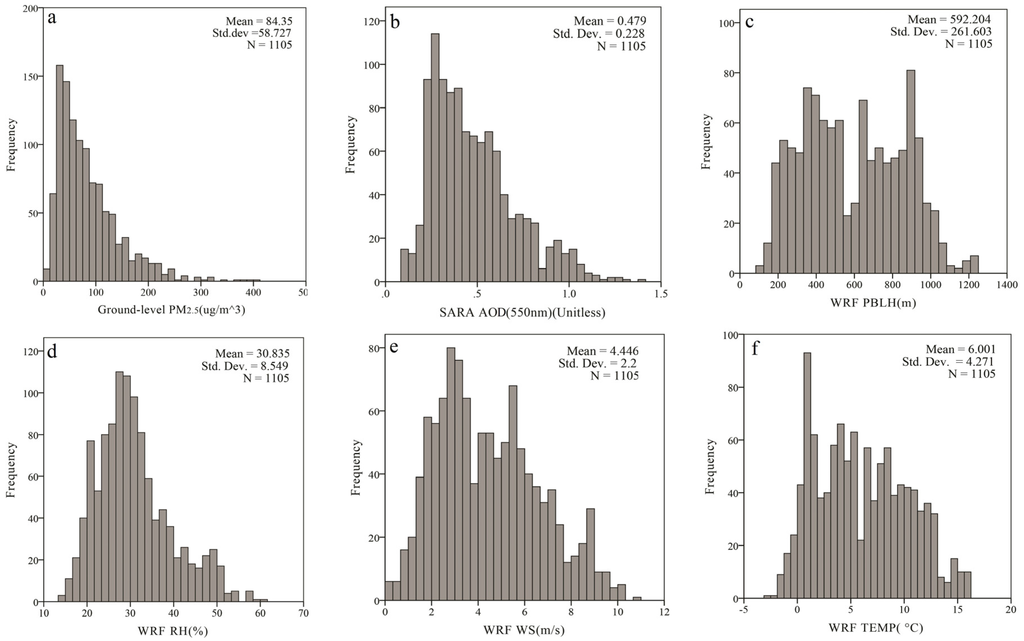
Figure 2.
Histograms and descriptive statistics of six variables ((a) Ground-level PM2.5; (b) SARA AOD; (c) WRF PBLH; (d) WRF RH; (e) WRF WS; and (f) WRF TEMP).
For further understanding the response of ground level PM2.5 concentrations to meteorological condition changes, the LOESS (locally weighted polynomial regression) trend lines were added in the scatter-plots between ground level PM2.5 and the predictors in SPSS (Figure 3). LOESS combines the simplicity of linear least squares regression with the flexibility of nonlinear regression and fits simple models to localized subsets of the data [42]. It shows that SARA AOD and RH seems to be significantly associated with ground level PM2.5 concentration in a nearly positive linear model (Figure 3a,c), while PBLH and WS fit with a nearly negative linear model (Figure 3b,d). Ground-level PM2.5 concentration increases when the TEMP is below around 7 °C, but decreases as the temperature gets higher than 7 °C (Figure 3e).
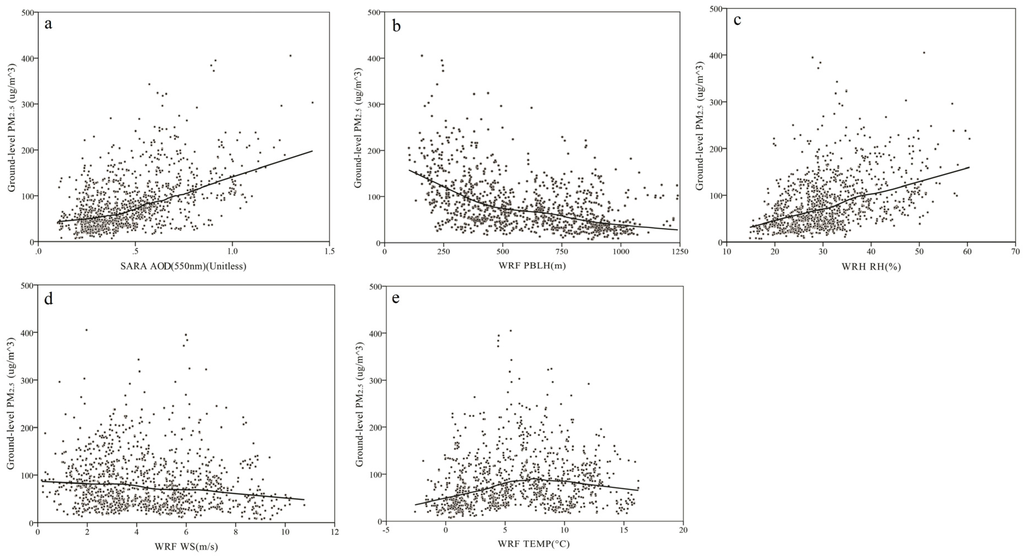
Figure 3.
Scatter plots of the meteorological fields ((a) SARA AOD; (b) WRF PBLH; (c) WRF RH; (d) WRF WS; and (e) WRF TEMP) against the hourly ground level PM2.5 concentration.
2.3. Methodology
2.3.1. Geographically and Temporally Weighted Regression (GTWR) Model
Compared with traditional linear or nonlinear regression methods, the GWR model, as one of the spatial varying coefficient regression models, can significantly improve the estimation accuracy of ground-level PM2.5, especially in a study region with a complex spatial context. Furthermore, Huang et al. [43] developed a GTWR model to deal with the spatial and temporal non-stationarity issues simultaneously through incorporating temporal effects into the GWR model. In this article, to effectively delineate the spatio-temporal quantitative relationship between satellite-derived AOD, coupled with meteorological data, and ground-level PM2.5 concentrations at the regional scale, a GTWR model was developed to improve the local coefficient of determination parameter (R2) for satellite-derived AOD and ground PM2.5 measurements on hourly basis.
Supposing the sample is labeled as , the GTWR model for the PM2.5–AOD relationship can be mathematically expressed as:
where represents the given coordinates of the training sample in space at time ; is the intercept value; , , , , and denote the slope of AOD, PBLH, RH, TEMP, and WS, respectively; and stands for the random error. The meteorological variables are used as sensitive factors to improve the association between satellite-derived AOD and ground-level PM2.5 concentrations because the RH and TEMP can be employed for indicating the changes in particle compositions and the PBLH and WS influence the vertical profile of particulate matters.
In order to calibrate the parameters in the GTWR model, a local weighted least squares algorithm is usually employed, assuming that the closer the measurements to point in space-time coordinate system, the greater the weight the measurements have in predicting . Thus, the estimation of parameters is expressed as:
where is a square matrix computing the geographical and temporal weighted values of training datasets for measurement by the diagonal elements, and the parameter is a vector representing the parameters AOD, PBLH, RH, TEMP, and WS.
Considering the different scale effects of location and time, an ellipsoidal coordinate system was used to measure the spatio-temporal distance between a regressive point and its surrounding measurement data. Through combining the temporal distance with the spatial distance , the spatio-temporal distance is defined as:
where denotes different kinds of operators. Moreover, Gaussian distance decay-based functions and Euclidean distance were chosen to construct the spatio-temporal weight matrix, and the “+” operator was adopted to assess the space-time distance . As a result, the and the diagonal element of weight matrix can be obtained as follows:
where is a non-negative parameter known as bandwidth, which produces a decay of influence with distance.
2.3.2. Statistical Analysis
Some statistical indicators were employed to evaluate the estimation accuracy of GTWR model through comparing the fitted PM2.5 concentration with ground PM2.5 measurements, such as R2, root mean square error (RMSE), mean absolute difference (MAD), and mean absolute percentage error (MAPE). The R2 of a statistical model is an indicator describing the discrepancy between ground-observed PM2.5 and satellite-estimated ground-level PM2.5, where higher values indicate better fitting accuracy. The R2 is defined as:
where is the number of ground measurement; and stand for the original and averaged concentration of ground-observed PM2.5, respectively; and stands for the concentration of satellite-estimated ground-level PM2.5.
The RMSE is employed to measure the differences between ground-observed PM2.5 and satellite estimated ground-lever PM2.5, which is sensitive to both systematic error and random error. The RMSE is calculated as:
The MAD used to measure the magnitude of mean error magnitude is computed as:
The MAPE expressing estimation accuracy of a statistical model as a percentage is defined by:
2.3.3. Implementation of the Proposed Method
Figure 4 presents a flowchart of the proposed estimating method. The Terra/Aqua MODIS level-1 and level-2 products with aerosol properties, including SSA and asymmetry parameter obtained from AERONET, are first employed to generate AOD images with 500 m spatial resolution at the satellite overpassing moment based on SARA. Then, meteorological field images including PBLH, RH, WS, and TEMP are extracted from WRF assimilation, and are geo-registered and interpolated to the same coordinate system and the same spatial resolution of SARA AOD by using a cubic spline interpolation algorithm. Finally, hourly PM2.5 concentration maps at 500 m resolution were produced using SARA AOD products and meteorological field datasets with four models including GTWR, ordinary OLS, GWR, and the TWR model, respectively. Only the data spatially co-located at the selected 37 ground stations and temporally matched with MODIS overpassing moments were included in the following analyses. More details are given in Table 1.
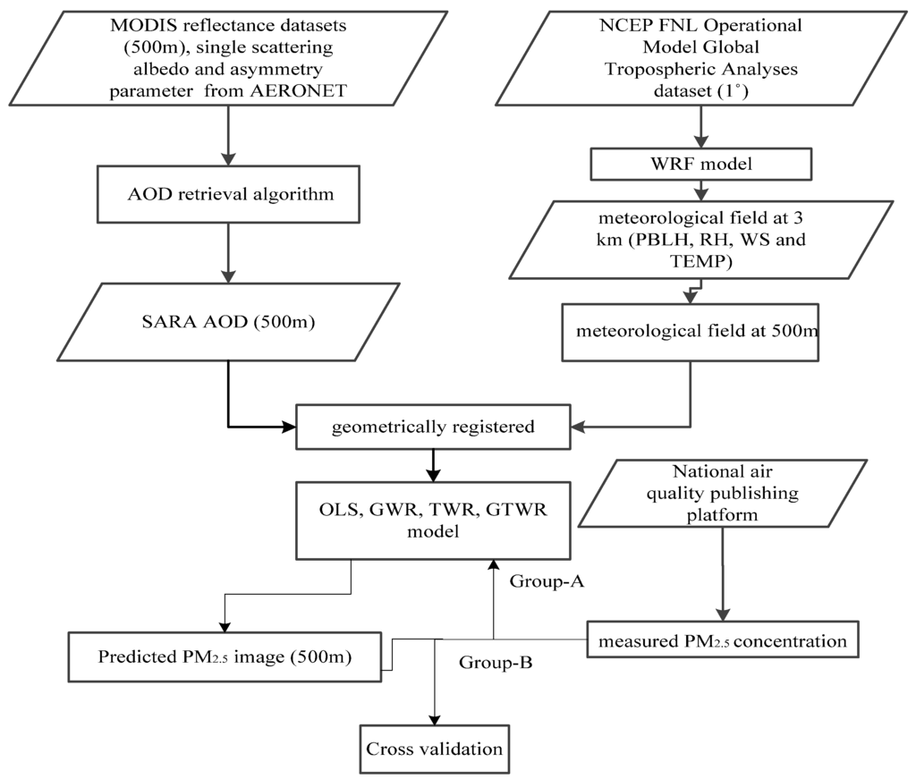
Figure 4.
Flowchart of the proposed GTWR method for estimating hourly PM2.5 at 500 m resolution.

Table 1.
A summary of data variables used in the GTWR model.
3. Modeling Results and Discussions
3.1. SARA AOD and Quality Contrast
In this study, MODIS Terra/Aqua satellite products were used to generate Terra/Aqua SARA AOD using XuZhou-CUMT AERONET data. High AOD values, 0.60 and 0.71 at 0.55 μm, were observed on 11 January 2015 and 13 February 2015, respectively, during the MODIS Terra/Aqua overpass moments at XuZhou-CUMT AERONET station. Figure 5d and Figure 6d show the image of SARA AOD with 500 m resolution over the studied area on the haze days. Furthermore, MODIS Dark Target (DT) and MODIS Deep Blue (DB) AOD products at 0.55 μm were also obtained to compare with the SARA AOD. For both Terra and Aqua satellites, MODIS DT algorithm (Figure 5b and Figure 6b) has many missing pixels and is incapable of retrieving AOD fully during the haze events owing to its selection of dark pixels when the observed MOD09 surface reflectance product at 2.21 μm is larger than 0.30 over the study region. Although the MODIS DB algorithm (Figure 5c and Figure 6c) has fewer missing pixels and is able to retrieve AOD during the haze events as compared to the MODIS DT algorithm, the retrieved AOD has coarser spatial resolution than SARA AOD. The contrast shows that both MODIS DT and DB algorithms obtained a relatively high estimation of regional AOD, while SARA AOD obtained approximate values referring to ground-based AERONET AOD. In other words, SARA AOD not only displays similar spatial distribution pattern with MODIS DT/DB AOD over the study region, but also provides better accuracy and more details during the haze events. Hence the SARA AOD of 500 m spatial resolution is more suitable for studies on environmental problems since many studies need population-related PM2.5 exposure information of a polluted factory or residential quarter.
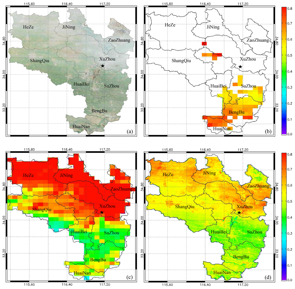
Figure 5.
Contrast of satellite-derived AOD results in the study region on 11 January 2015. (a) True color (RGB:143); (b) Terra DT AOD at 10 km; (c) Terra DB AOD at 10 km; (d) Terra SARA AOD at 500 m.
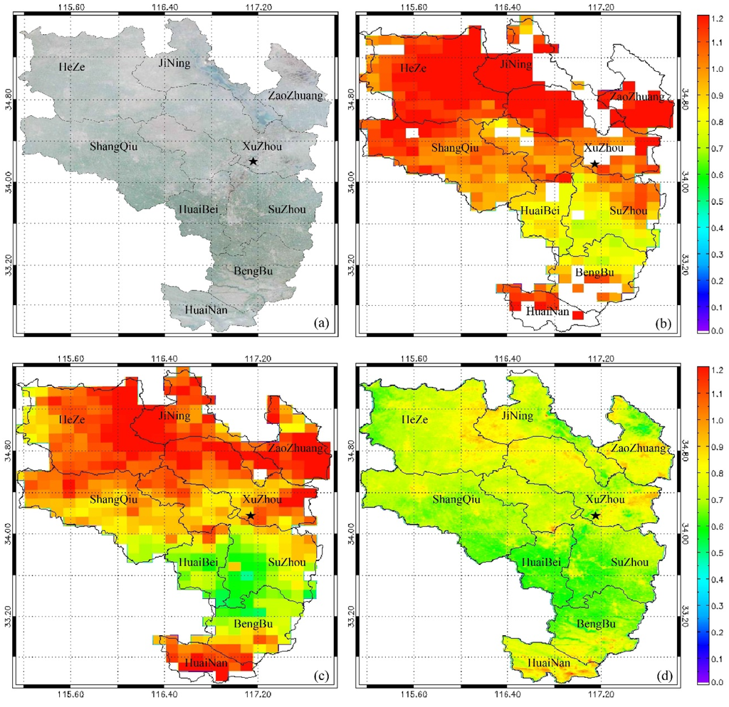
Figure 6.
Contrast of satellite-derived AOD results in the study region on 13 February 2015. (a) True color (RGB:143); (b) Aqua DT AOD at 10 km; (c) Aqua DB AOD at 10 km; (d) Aqua SARA AOD at 500 m.
3.2. Comparison between Fitted and Ground-Observed PM2.5
Hourly PM2.5 concentration values and matched estimations were obtained at the 37 monitoring stations in which regional haze episodes have occurred frequently over the study region from 1 November 2014 to 28 February 2015. About two-thirds of the observed measurements (group-A) extracted from each city is used as training dataset (N = 700) for model fitting and the other one-thirds (group-B) is used as a validation dataset (N = 405) for cross validation. For example if the number of monitoring stations in a city is three or four, the observed data points from the one selected station are used as validation datasets and the observed data points from the remaining two or three stations will be used as training datasets. The OLS, GWR, TWR, and GTWR models were tested using the same datasets. Unlike the OLS method, which directly uses numerical values of variables without any spatial or temporal considerations (taking space coordinates and time as exogenous determinants), the GWR model extends the traditional regression framework for dealing with spatial non-stationarity when different relationships exist at different points in space, and TWR integrates the temporal information in the weighting matrices to capture the temporal heterogeneity when different relationships exist at the same points in time. The results of the model fitting and cross validation are reported in Table 2 and Table 3.
Table 2.
Quantitative assessment of model fitting via OLS, GWR, TWR, and GTWR.
Table 3.
Quantitative assessment of cross-validation via OLS, GWR, TWR, and GTWR.
The tables show that the R2 of GTWR (0.96 and 0.87) is two times more than that of OLS (0.35 and 0.41), while the R2 of TWR (0.63 and 0.68) is a little bigger than that of GWR (0.59 and 0.60) both in model fitting and cross validation processes. Although the GTWR model is a bit over-fitting, i.e., R2 decreased 0.09 from model fitting to cross validation, the GTWR obtained the highest value of R2 in the cross-validation process. Furthermore, the GTWR model shows RMSEs of 11.47 μg/m3 and 21.77 μg/m3, and MAD of 6.91 μg/m3 and 12.92 μg/m3 for model fitting and cross validation, respectively, between the ground-observed PM2.5 and the fitted PM2.5 concentrations. It shows also the PM2.5 data estimated from the GTWR model agree well with the ground measurements, indicating that the spatial and temporal variation of model parameters should be considered in the PM2.5–AOD relationship.
Additionally, approximately 10.8% and 23.2% of the GTWR PM2.5 estimation errors are obtained from model fitting and cross validation, respectively, which are far lower than those of the other three models. This proves the ability of the GTWR model to estimate ground-level PM2.5 concentrations from MODIS SARA-AOD. The comparisons indicate that GTWR is able to accurately capture the spatio-temporal variability of the PM2.5–AOD relationship, and the PM2.5 estimations agree well with the ground measurements over the study region even if haze episodes occur frequently.
To further evaluate the performance of the GTWR model, all the PM2.5 measurements from 37 monitoring stations were used as a training dataset (N = 1105). Figure 7 quantitatively illustrates the mean difference between the GTWR estimations and ground measurements at 37 monitoring stations. It shows that the GTWR estimations agree well with the ground measurements. The PM2.5 discrepancies vary from 6.61 μg/m3 (as the ground measurement is 38.35 μg/m3) to −11.72 μg/m3 (as the ground measurement is 117.79 μg/m3). Around 94.6% of the GTWR estimations correlate well with ground measurements at very low discrepancies (e.g., with the error less than 4.0 μg/m3).
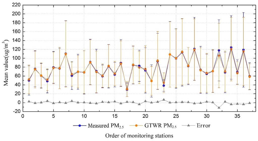
Figure 7.
Comparison between GTWR estimations and ground measurements of PM2.5 concentration.
Figure 8 and Figure 9 give the scatter plots between measured and fitted PM2.5 concentrations with OLS, GWR, TWR, and GTWR model, respectively. All the slopes (0.35, 0.56, 0.61, and 0.94 for model fitting, and 0.38, 0.57, 0.63, and 0.89 for cross validation, respectively, for the OLS, GWR, TWR, and GTWR models) of the above four models are smaller than 1. This characteristic implies that most of the PM2.5 concentrations are systematically underestimated both in model fitting and cross validation. Figure 8a and Figure 9a show that few estimations of OLS (r = 0.60 and 0.65 for fitting and validation, respectively) lie close to the 1:1 line, and a wide scattering of points is seen due to underestimation and overestimation. Figure 8b and Figure 9c show that the GWR estimations have comparable correlation coefficients (r = 0.77 and 0.80 for fitting and validation, respectively) with TWR estimations, and the r of both GWR and TWR are greater than OSL. This tells us that spatial and temporal variability should be considered in the linear regression model. Figure 8d and Figure 9d show that the majority of the GTWR estimations (r = 0.98 and 0.93 for fitting and validation, respectively) are close to the 1:1 line and fall in the 95% confidence envelope. They also show that when the ground measurement is lower than 100 μg/m3, the estimations have a relatively good quality except for OLS; when the ground measurements become larger than 150 μg/m3, the performance of GTWR is far better than the other three models. In a word, the GTWR model displays the best performance both for model fitting and cross validation.
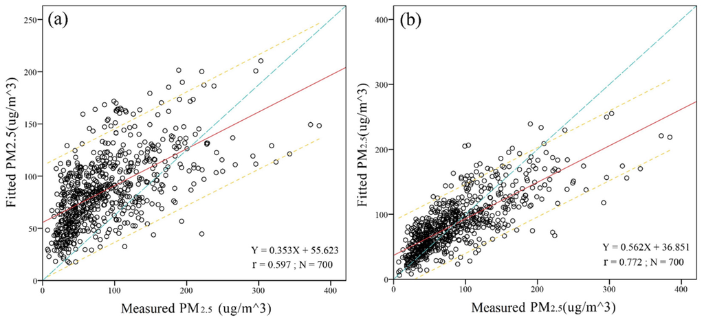
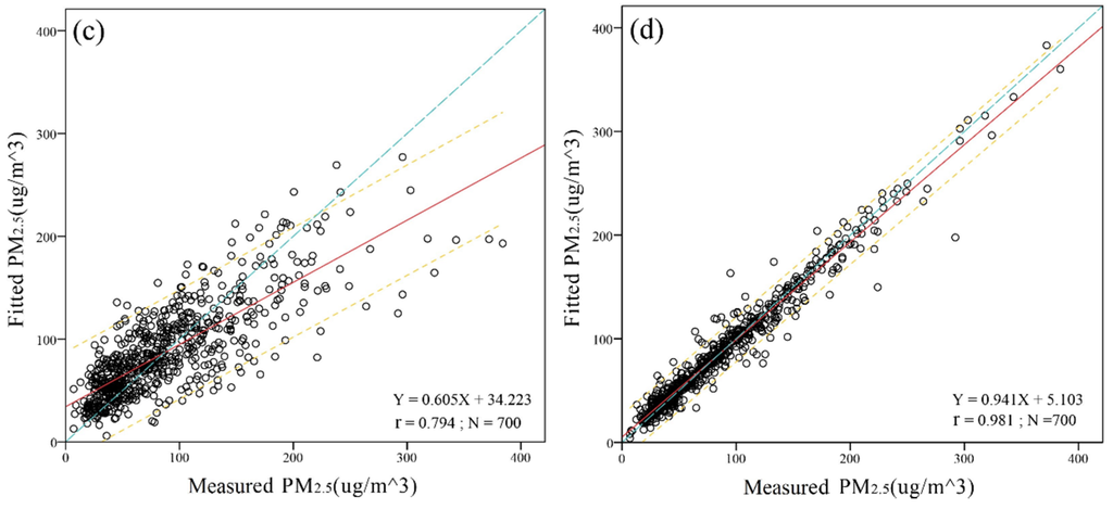
Figure 8.
Scatter plots between the measured and fitted PM2.5 concentrations for model fitting. (a) OLS; (b) GWR; (c) TWR; and (d) GTWR. The short dashed (orange) line, long dashed (blue) line, and solid (red) line are the 95% confidence band, 1:1 line, and regression line, respectively.
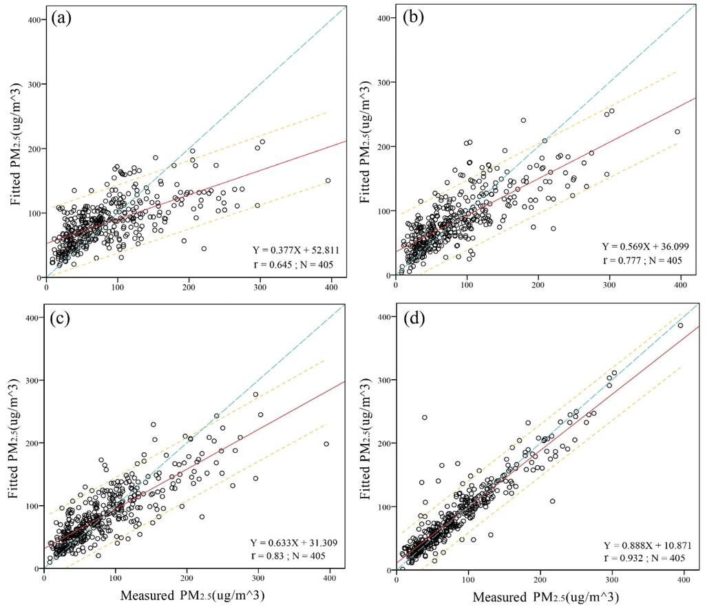
Figure 9.
Scatter plots between the measured and fitted PM2.5 concentrations for cross validation. (a) OLS; (b) GWR; (c) TWR and (d) GTWR. The short dashed (orange) lines, long dashed (blue) line, and solid (red) line are the 95% confidence band, 1:1 line, and regression line, respectively.
3.3. Spatio-Temporal Distribution of AOD-Estimated PM2.5 with GTWR
Figure 10 illustrate the spatio-temporal distribution of PM2.5 hourly concentrations estimated from MODIS SARA-AOD with GTWR model during a haze formation process from the afternoon of 8 February 2015 to the morning of 11 February 2015. On 8 February 2015, the pollution is concentrated over HeZe, ShangQiu, and the west part of JiNing with PM2.5 concentrations ranging from 60 μg/m3 to 70 μg/m3 when the other six cities are not yet polluted (Figure 10a from Aqua). Then, the pollution is extended to the south and east, and brings higher PM2.5 to ZaoZhuang, Xuzhou, and the northwest of SuZhou (Figure 10b–e for 9 February 2015 and 10 February 2015). Up to 11 February 2015, the extremely high pollution is centered at ZaoZhuang, JiNing, and the northeast part of HeZe, with PM2.5 concentrations beyond 150 μg/m3. This shows that the PM2.5 concentrations over the study region slowly accumulated during this haze process except for the dramatic increase in ZaoZhuang and JiNing, which indicates that both local and external pollutant sources had an impact on the PM2.5 concentration.
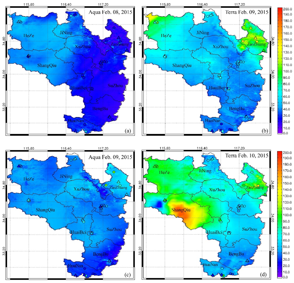
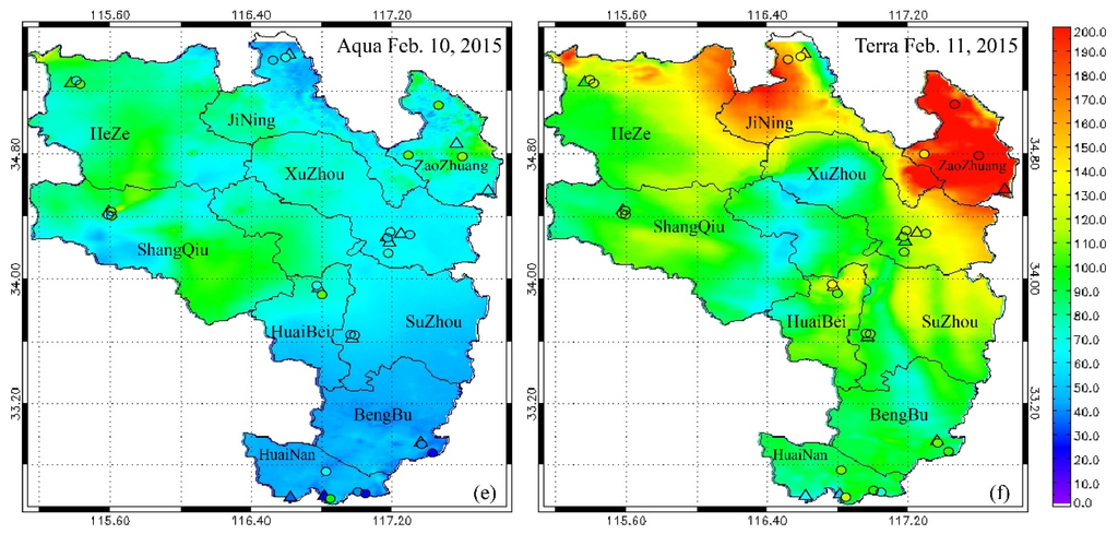
Figure 10.
Spatial distribution of GTWR model-estimated PM2.5 concentration, from Terra (local time 10:30 a.m.) and Aqua (local time 1:30 p.m.), respectively, over the study region during a haze formation process from the afternoon of 8 February 2015 to the morning of 11 February 2015 ((a) Aqua 8 February 2015; (b) Terra 9 February 2015; (c) Aqua 9 February 2015; (d) Terra 10 February 2015; (e) Aqua 10 February 2015; and (f) Terra 11 February 2015). In situ measurements at training stations (circles) and validation (triangles) stations are also shown in the figures.
Furthermore, it shows that the AOD-estimated PM2.5 concentration from Terra at about 10:30 a.m. is higher than that from Aqua at about 1:30 p.m. in the same day, and these temporal characteristics agree with the ground measurements over the study region (Figure 10b,c on 9 February 2015, and Figure 10d,e on 10 February 2015). Moreover, more spatial details and higher estimation accuracy are obtained near the monitoring stations. That is to say, if there are more ground measurements with spatial homogeneous distribution over the study region, the estimation accuracy of the GTWR model can be improved further.
The AOD-estimated PM2.5 images with GTWR model are also compared with spatially interpolated ground measurements (Figure 11) with the ordinary Kriging method. The ground measurements can be regarded as relatively independent and the ordinary Kriging method is well proved in the literature [45,46], being more suitable than the inverse distance weighted (IDW) and three splines (TS) methods embodied in ArcGIS, in that the ground measurements are obtained from sparse and irregularly distributed air quality monitoring stations. Although the spatio-temporal patterns of ordinary Kriging-interpolated PM2.5 measurements are roughly similar to those of GTWR-estimated PM2.5 concentration, the former have poor accuracy and less spatial details in places far from the monitoring stations, which might be attributable to the following reasons: (i) The ordinary Kriging-interpolated PM2.5 concentrations cannot exceed the maximum and minimum values of the ground measurements (e.g., the southeast of ShangQiu on 10 February 2015 and the northwest of XuZhou on 11 February); (ii) the coarse spatial coverage and irregular distribution of ground stations may introduce certain estimation errors into the ordinary Kriging method.
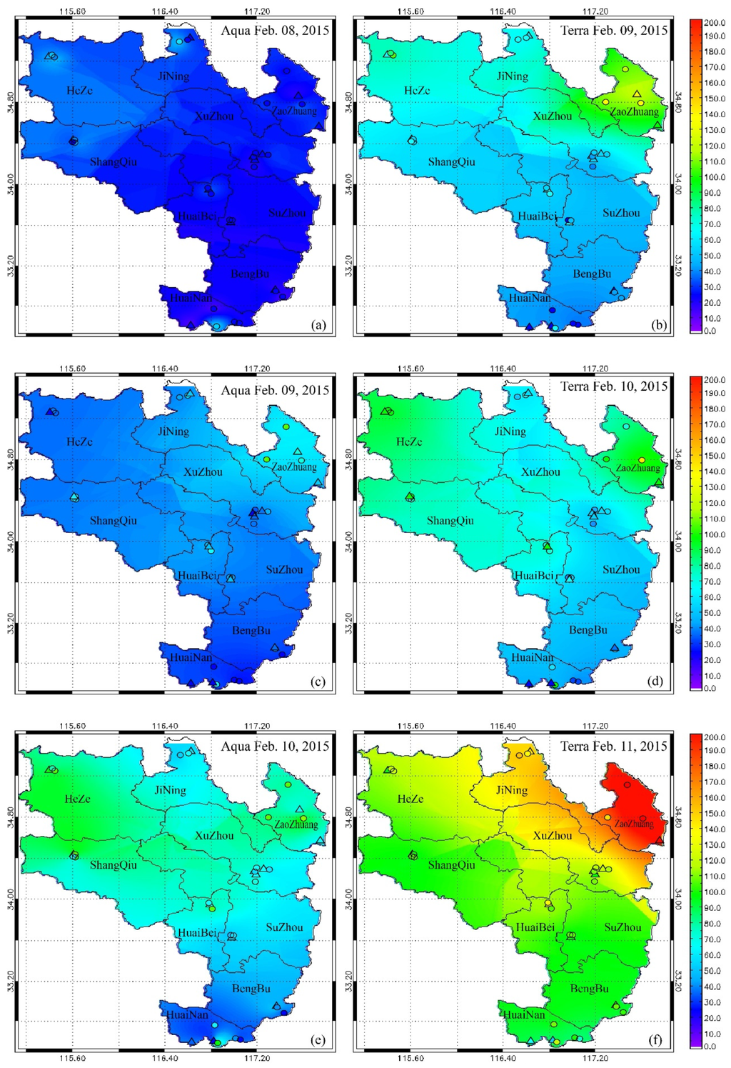
Figure 11.
Spatial distribution of ground PM2.5 measurements over the study region during a haze formation process from the afternoon of 8 February 2015 to the morning of 11 February 2015, referring to the local passing moment of satellites Terra and Aqua ((a) Aqua 8 February 2015; (b) Terra 9 February 2015; (c) Aqua 9 February 2015; (d) Terra 10 February 2015; (e) Aqua 10 February 2015; and (f) Terra 11 February 2015). In situ measurements at training stations (circles) and validation (triangles) stations are also shown in the figures.
In conclusion, GTWR is capable of estimating ground-level PM2.5 concentrations with good accuracy in regions lacking ground measurements but with satellite AOD available, and the estimated PM2.5 images can display the detailed spatial patterns and dynamic evolution process of regional PM2.5 concentrations.
3.4. Discussions
The GTWR model was employed to depict the relationship between satellite-derived AOD and ground-level PM2.5 concentrations during the period between November 2014 and February 2015. The proposed GTWR model and estimation method in this paper has several benefits over the conventional statistical models used in previous studies.
Firstly, we use high spatial resolution SARA AOD of 500 m resolution to estimate ground-level PM2.5 concentrations. Compared to ground-observed AOD from AERONET, the SARA AOD has much higher estimation accuracy than that from MODIS 04 algorithm during fine-particle pollution events [47], which indicates that SARA AOD is more suitable for estimating ground-level PM2.5 concentrations. On the other hand, SARA AOD has a considerably larger spatial coverage than MODIS DT/DB AOD over areas with high surface reflectance or undergoing a haze episode. Therefore, the SARA-retrieved 500 m AOD and GTWR-estimated ground-level PM2.5 concentrations can be utilized to monitor the urban air pollution status at a finer spatio-temporal scale.
Secondly, we use four models to depict the spatio-temporal dynamics in the relationships between satellite-retrieved AOD and ground-level PM2.5 estimations. From Table 2 and Table 3, we know that the estimation accuracy of TWR is higher than GWR, implying that the temporal non-stationarity has a more significant impact on model fitting based on the training datasets than spatial non-stationarity in this case study, which may be attributable to the following reasons: (i) in order to monitor the daily dynamic of air quality, the observations from MODIS TERRA and AQUA sensors are input to the statistic models for estimating ground-level PM2.5 concentrations; (ii) haze episodes occur frequently in winter, resulting in low AOD value but high PM2.5 concentrations; (iii) the topography and land use in the study region are pretty much even, without dramatic differences. The GTWR model allows for hourly-to-hourly variability in the PM2.5–AOD relationship by incorporating temporal effects into the GWR model. The lowest RMSE values and the high correlation coefficients from GTWR-based estimation illustrate that the fitted and observed PM2.5 have a strong relationship (Figure 8 and Figure 9).
Thirdly, we use hourly assimilated meteorological field data including PBLH, RH, TEMP, and WS extracted from WRF assimilation as auxiliary data to improve the estimation accuracy. The good performance of the GTWR-based estimation method shows that ground-observed meteorological field data can be substituted for simulated meteorological field datasets if hourly ground meteorological observations are lacking.
4. Conclusions
In this study, a GTWR model was proposed to incorporate the geographical difference and temporal variation of the PM2.5–AOD relationship, and to estimate ground-level PM2.5 concentration from satellite-retrieved AOD products. SARA AOD of 500 m resolution is produced from MODIS observations and input to the GTWR model together with assimilated meteorological data, including the PBLH, RH, WS, and TEMP from the WRF model, to estimate ground-level PM2.5 concentration. Other models such as OLS, GWR, and TWR were applied for comparison with a common case study in central China. This showed that the GTWR model produces the highest R2 and r values as well as the lowest RMSE, MAD, and MAPE values among the four models. GTWR provides a simple but effective method of estimating hourly ground-level PM2.5 concentrations at 500 m spatial resolution, and can substantially increase the estimation accuracy. The estimations are valuable for urban- and regional-scale air quality monitoring and government decision-making, especially for rural regions lacking ground measurements.
However, some limitations/errors remain in GTWR estimation because (i) no effective method is applied to fill the gaps in pixels where AOD is not retrieved due to SARA being unable to estimate AOD in missing pixels caused by the presence of thick clouds; (ii) no finer correction is made with LUCC data when a pixel involves water surface; (iii) the pixels covered by snow are temporally suggested to be ignored and set to null values in the current model and the model will be improved to be accountable for this special situation; (iv) the ground PM2.5 monitoring stations are limited and irregularly distributed, which may reduce the estimation accuracy in areas far from stations; (v) it is effective in cases where the near-surface aerosol is the dominant load in the vertical direction, but will not work in long-range transported aerosol episodes such as dust storms for its entrance to the middle troposphere, when the-satellite observed AOD becomes less relevant to surface PM2.5 concentration; and (vi) the spatial resolution and accuracy of meteorological field data simulated in the WRF model are not good enough. Future strategies for improvement include: (i) ground-level PM2.5 estimation from other high spatial resolution satellite sensors, such as Landsat and HJ-1A, for the study of microenvironments of human exposure (e.g., coal mining areas, power plants, business quarters, and residential areas); (ii) more factors such as land use, wind direction, and fire product being cooperated in the GTWR model; (iii) physical and chemical properties of aerosol particulates being explored for PM2.5 estimation; and (iv) air quality models such as temporal gap-filling being coupled with the GTWR model to estimate ground-level PM2.5 concentrations at nighttime and in pixels where the AOD retrieval is not valid for a given day.
Acknowledgments
This research was sponsored by the grant KYLX15_1435 from the Funding of Jiangsu Innovation Program for Graduate Education, grant 2014QNA32 from the Fundamental Research Funds for the Central Universities, and the project funded by the Priority Academic Program Development (PAPD) of Jiangsu Higher Education Institutions. We would also like to thank the NASA Goddard Space Flight Center for providing MODIS images, and the MAESTRO (Mining Area Environment Synergic observaTion pRoving ground) program of CUMT for providing AERONET data.
Author Contributions
Yai Bai, Lixin Wu, and Yangyang Shen conceived and designed the experiments, performed the experiments, and analyzed the data; Yai Bai, Lixin Wu, Kai Qin, Yufeng Zhang, Yangyang Shen, and Yuan Zhou prepared the manuscript; and Lixin Wu improved the ideas and made revisions.
Conflicts of Interest
The authors declare no conflict of interest.
References
- Evans, J.; van Donkelaar, A.; Martin, R.V.; Burnett, R.; Rainham, D.G.; Birkett, N.J.; Krewski, D. Estimates of global mortality attributable to particulate air pollution using satellite imagery. Environ. Res. 2013, 120, 33–42. [Google Scholar] [CrossRef] [PubMed]
- Watterson, T.L.; Sorensen, J.; Martin, R.; Coulombe, R.A., Jr. Effects of PM2.5 collected from cache valley utah on genes associated with the inflammatory response in human lung cells. J. Toxicol. Environ. Health A Curr. Issues 2007, 70, 1731–1744. [Google Scholar] [CrossRef] [PubMed]
- Lepeule, J.; Laden, F.; Dockery, D.; Schwartz, J. Chronic exposure to fine particles and mortality: An extended follow-up of the Harvard six cities study from 1974 to 2009. Environ. Health Perspect. 2012, 120, 965–970. [Google Scholar] [CrossRef] [PubMed]
- Boldo, E.; Medina, S.; LeTertre, A.; Hurley, F.; Muecke, H.-G.; Ballester, F.; Aguilera, I.; Eilstein, D.; Apheis, G. Apheis: Health impact assessment of long-term exposure to PM2.5 in 23 European cities. Eur. J. Epidemiol. 2006, 21, 449–458. [Google Scholar] [CrossRef] [PubMed]
- Pope, C.A.; Burnett, R.T.; Thun, M.J.; Calle, E.E.; Krewski, D.; Ito, K.; Thurston, G.D. Lung cancer, cardiopulmonary mortality, and long-term exposure to fine particulate air pollution. J. Am. Med. Assoc. 2002, 287, 1132–1141. [Google Scholar] [CrossRef]
- Chan, C.K.; Yao, X. Air pollution in mega cities in China. Atmos. Environ. 2008, 42, 1–42. [Google Scholar] [CrossRef]
- Chu, H.J.; Huang, B.; Lin, C.Y. Modeling the spatio-temporal heterogeneity in the PM10–PM2.5 relationship. Atmos. Environ. 2015, 102, 176–182. [Google Scholar] [CrossRef]
- Hua, Y.; Cheng, Z.; Wang, S.; Jiang, J.; Chen, D.; Cai, S.; Fu, X.; Fu, Q.; Chen, C.; Xu, B. Characteristics and source apportionment of pm2.5 during a fall heavy haze episode in the Yangtze River Delta of China. Atmos. Environ. 2015, 123, 380–391. [Google Scholar] [CrossRef]
- Song, L.; Pang, S.; Longley, I.; Olivares, G.; Sarrafzadeh, A. Spatio-Temporal PM2.5 Prediction by Spatial Data Aided Incremental Support Vector Regression. In Proceedings of the 2014 International Joint Conference on Neural Networks (IJCNN), Beijing, China, 6–11 July 2014; pp. 623–630.
- Van Donkelaar, A.; Martin, R.V.; Park, R.J. Estimating ground-level PM2.5 using aerosol optical depth determined from satellite remote sensing. J. Geophys. Res. Atmos. 2006, 111. [Google Scholar] [CrossRef]
- Kloog, I.; Koutrakis, P.; Coull, B.A.; Lee, H.J.; Schwartz, J. Assessing temporally and spatially resolved PM2.5 exposures for epidemiological studies using satellite aerosol optical depth measurements. Atmos. Environ. 2011, 45, 6267–6275. [Google Scholar] [CrossRef]
- Van Donkelaar, A.; Martin, R.V.; Brauer, M.; Kahn, R.; Levy, R.; Verduzco, C.; Villeneuve, P.J. Global estimates of ambient fine particulate matter concentrations from satellite-based aerosol optical depth: Development and application. Environ. Health Perspect. 2010, 118, 847–855. [Google Scholar] [CrossRef] [PubMed]
- Hu, X.; Waller, L.A.; Lyapustin, A.; Wang, Y.; Al-Hamdan, M.Z.; Crosson, W.L.; Estes, M.G.; Estes, S.M.; Quattrochi, D.A.; Puttaswamy, S.J. Estimating ground-level PM2.5 concentrations in the southeastern United States using MAIAC AOD retrievals and a two-stage model. Remote Sens. Environ. 2014, 140, 220–232. [Google Scholar] [CrossRef]
- Hu, Z. Spatial analysis of MODIS aerosol optical depth, PM2.5, and chronic coronary heart disease. Int. J. Health Geogr. 2009, 8, 27. [Google Scholar] [CrossRef] [PubMed]
- Strawa, A.W.; Chatfield, R.B.; Legg, M.; Scarnato, B.; Esswein, R. Improving retrievals of regional fine particulate matter concentrations from moderate resolution imaging spectroradiometer (MODIS) and ozone monitoring instrument (OMI) multisatellite observations. J. Air Waste Manag. Assoc. 2013, 63, 1434–1446. [Google Scholar] [CrossRef] [PubMed]
- Van Donkelaar, A.; Martin, R.V.; Levy, R.C.; da Silva, A.M.; Krzyzanowski, M.; Chubarova, N.E.; Semutnikova, E.; Cohen, A.J. Satellite-based estimates of ground-level fine particulate matter during extreme events: A case study of the Moscow fires in 2010. Atmos. Environ. 2011, 45, 6225–6232. [Google Scholar] [CrossRef]
- You, W.; Zang, Z.L.; Pan, X.B.; Zhang, L.F.; Chen, D. Estimating PM2.5 in Xi’an, china using aerosol optical depth: A comparison between the MODIS and MISR retrieval models. Sci. Total Environ. 2015, 505, 1156–1165. [Google Scholar] [CrossRef] [PubMed]
- Liu, Y.; Koutrakis, P.; Kahn, R.; Turquety, S.; Yantosca, R.M. Estimating fine particulate matter component concentrations and size distributions using satellite-retrieved fractional aerosol optical depth: Part 2—A case study. J. Air Waste Manag. Assoc. 2007, 57, 1360–1369. [Google Scholar] [PubMed]
- Weber, S.A.; Engel-Cox, J.A.; Hoff, R.M.; Prados, A.I.; Zhang, H. An improved method for estimating surface fine particle concentrations using seasonally adjusted satellite aerosol optical depth. J. Air Waste Manag. Assoc. 2010, 60, 574–585. [Google Scholar] [CrossRef] [PubMed]
- Liu, Y.; Paciorek, C.J.; Koutrakis, P. Estimating regional spatial and temporal variability of PM2.5 concentrations using satellite data, meteorology, and land use information. Environ. Health Perspect. 2009, 117, 886–892. [Google Scholar] [CrossRef] [PubMed]
- Paciorek, C.J.; Liu, Y. Assessment and statistical modeling of the relationship between remotely sensed aerosol optical depth and PM2.5 in the eastern United States. Res. Rep. (Health Eff. Inst.) 2012, 167, 5–83, discussion 85–91. [Google Scholar] [PubMed]
- Reid, C.E.; Jerrett, M.; Petersen, M.L.; Pfister, G.G.; Morefield, P.E.; Tager, I.B.; Raffuse, S.M.; Balmes, J.R. Spatiotemporal prediction of fine particulate matter during the 2008 northern California wildfires using machine learning. Environ. Sci. Technol. 2015, 49, 3887–3896. [Google Scholar] [CrossRef] [PubMed]
- Kumar, N.; Chu, A.; Foster, A. An empirical relationship between PM2.5 and aerosol optical depth in Delhi metropolitan. Atmos. Environ. 2007, 41, 4492–4503. [Google Scholar] [CrossRef] [PubMed]
- Xin, J.Y.; Zhang, Q.; Wang, L.L.; Gong, C.S.; Wang, Y.S.; Liu, Z.R.; Gao, W.K. The empirical relationship between the PM2.5 concentration and aerosol optical depth over the background of North China from 2009 to 2011. Atmos. Res. 2014, 138, 179–188. [Google Scholar] [CrossRef]
- Engel-Cox, J.A.; Holloman, C.H.; Coutant, B.W.; Hoff, R.M. Qualitative and quantitative evaluation of MODIS satellite sensor data for regional and urban scale air quality. Atmos. Environ. 2004, 38, 2495–2509. [Google Scholar] [CrossRef]
- Tian, J.; Chen, D. A semi-empirical model for predicting hourly ground-level fine particulate matter (PM2.5) concentration in southern Ontario from satellite remote sensing and ground-based meteorological measurements. Remote Sens. Environ. 2010, 114, 221–229. [Google Scholar] [CrossRef]
- Sorek-Hamer, M.; Strawa, A.W.; Chatfield, R.B.; Esswein, R.; Cohen, A.; Broday, D.M. Improved retrieval of PM2.5 from satellite data products using non-linear methods. Environ. Pollut. 2013, 182, 417–423. [Google Scholar] [CrossRef] [PubMed]
- Kloog, I.; Chudnovsky, A.A.; Just, A.C.; Nordio, F.; Koutrakis, P.; Coull, B.A.; Lyapustin, A.; Wang, Y.J.; Schwartz, J. A new hybrid spatio-temporal model for estimating daily multi-year PM2.5 concentrations across northeastern USA using high resolution aerosol optical depth data. Atmos. Environ. 2014, 95, 581–590. [Google Scholar] [CrossRef]
- Saunders, R.O.; Kahl, J.D.W.; Ghorai, J.K. Improved estimation of PM2.5 using lagrangian satellite-measured aerosol optical depth. Atmos. Environ. 2014, 91, 146–153. [Google Scholar] [CrossRef]
- Zhou, Q.P.; Jiang, H.Y.; Wang, J.Z.; Zhou, J.L. A hybrid model for PM2.5 forecasting based on ensemble empirical mode decomposition and a general regression neural network. Sci. Total Environ. 2014, 496, 264–274. [Google Scholar] [CrossRef] [PubMed]
- Wu, Y.R.; Guo, J.P.; Zhang, X.Y.; Tian, X.; Zhang, J.H.; Wang, Y.Q.; Duan, J.; Li, X.W. Synergy of satellite and ground based observations in estimation of particulate matter in eastern China. Sci. Total Environ. 2012, 433, 20–30. [Google Scholar] [CrossRef] [PubMed]
- Paciorek, C.J.; Yang, L.; Hortensia, M.M.; Shobha, K. Spatiotemporal associations between goes aerosol optical depth retrievals and ground-level PM2.5. Environ. Sci. Technol. 2008, 42, 5800–5806. [Google Scholar] [CrossRef] [PubMed]
- Lee, H.J.; Liu, Y.; Coull, B.A.; Schwartz, J.; Koutrakis, P. A novel calibration approach of MODIS AOD data to predict PM2.5 concentrations. Atmos. Chem. Phys. 2011, 11, 7991–8002. [Google Scholar] [CrossRef]
- Hu, X.; Waller, L.A.; Al-Hamdan, M.Z.; Crosson, W.L.; Estes, M.G.; Estes, S.M.; Quattrochi, D.A.; Sarnat, J.A.; Liu, Y. Estimating ground-level PM2.5 concentrations in the southeastern U.S. Using geographically weighted regression. Environ. Res. 2013, 121, 1–10. [Google Scholar] [CrossRef] [PubMed]
- Song, W.; Jia, H.; Huang, J.; Zhang, Y. A satellite-based geographically weighted regression model for regional PM2.5 estimation over the Pearl River delta region in China. Remote Sens. Environ. 2014, 154, 1–7. [Google Scholar] [CrossRef]
- Li, J.; Carlson, B.E.; Lacis, A.A. How well do satellite AOD observations represent the spatial and temporal variability of PM2.5 concentration for the United States? Atmos. Environ. 2015, 102, 260–273. [Google Scholar] [CrossRef]
- Bilal, M.; Nichol, J.E.; Bleiweiss, M.P.; Dubois, D. A simplified high resolution MODIS aerosol retrieval algorithm (SARA) for use over mixed surfaces. Remote Sens. Environ. 2013, 136, 135–145. [Google Scholar] [CrossRef]
- Bilal, M.; Nichol, J.E.; Chan, P.W. Validation and accuracy assessment of a simplified aerosol retrieval algorithm (SARA) over Beijing under low and high aerosol loadings and dust storms. Remote Sens. Environ. 2014, 153, 50–60. [Google Scholar] [CrossRef]
- Zhang, Y. Online-coupled meteorology and chemistry models: History, current status, and outlook. Atmos. Chem. Phys. 2008, 8, 2895–2932. [Google Scholar] [CrossRef]
- Lee, J.; Shin, H.H.; Hong, S.Y.; Jimenez, P.A.; Dudhia, J.; Hong, J. Impacts of subgrid-scale orography parameterization on simulated surface layer wind and monsoonal precipitation in the high-resolution WRF model. J. Geophys. Res. Atmos. 2015, 120, 644–653. [Google Scholar] [CrossRef]
- Im, U.; Markakis, K.; Unal, A.; Kindap, T.; Poupkou, A.; Incecik, S.; Yenigun, O.; Melas, D.; Theodosi, C.; Mihalopoulos, N. Study of a winter PM episode in Istanbul using the high resolution WRF/CMAQ modeling system. Atmos. Environ. 2010, 44, 3085–3094. [Google Scholar] [CrossRef]
- Clevel, W.S.; Devlin, S.J. Locally weighted regression: An approach to regression analysis by local fitting. J. Am. Stat. Assoc. 1988, 83, 569–610. [Google Scholar]
- Huang, B.; Wu, B.; Barry, M. Geographically and temporally weighted regression for modeling spatio-temporal variation in house prices. Int. J. Geogr. Inf. Sci. 2010, 24, 383–401. [Google Scholar] [CrossRef]
- Fotheringham, A.S.; Charlton, M.E.; Brunsdon, C. Geographically weighted regression: A natural evolution of the expansion method for spatial data analysis. Environ. Plan. A Abstr. 1998, 30, 1905–1927. [Google Scholar] [CrossRef]
- Beelen, R.; Hoek, G.; Pebesma, E.; Vienneau, D.; Hoogh, K.D.; Briggs, D.J. Mapping of background air pollution at a fine spatial scale across the European union. Sci. Total Environ. 2009, 407, 1852–1867. [Google Scholar] [CrossRef] [PubMed]
- Perry, H.; Eleanor, S.; Alejandro, C.; Karla, P.; Steeve, D.; Michael, B.; Aaron, V.D.; Lok, L.; Randall, M.; Michael, J. Creating national air pollution models for population exposure assessment in Canada. Environ. Health Perspect. 2011, 119, 1123–1129. [Google Scholar]
- Bilal, M.; Nichol, J.E. Evaluation of MODIS aerosol retrieval algorithms over the Beijing-Tianjin-Hebei region during low to very high pollution events. J. Geophys. Res. Atmos. 2015, 120, 7941–7957. [Google Scholar] [CrossRef]
© 2016 by the authors; licensee MDPI, Basel, Switzerland. This article is an open access article distributed under the terms and conditions of the Creative Commons by Attribution (CC-BY) license (http://creativecommons.org/licenses/by/4.0/).