Abstract
Accurate land cover classification information is a critical variable for many applications. This study presents a method to classify land cover using the fusion data of airborne discrete return LiDAR (Light Detection and Ranging) and CASI (Compact Airborne Spectrographic Imager) hyperspectral data. Four LiDAR-derived images (DTM, DSM, nDSM, and intensity) and CASI data (48 bands) with 1 m spatial resolution were spatially resampled to 2, 4, 8, 10, 20 and 30 m resolutions using the nearest neighbor resampling method. These data were thereafter fused using the layer stacking and principal components analysis (PCA) methods. Land cover was classified by commonly used supervised classifications in remote sensing images, i.e., the support vector machine (SVM) and maximum likelihood (MLC) classifiers. Each classifier was applied to four types of datasets (at seven different spatial resolutions): (1) the layer stacking fusion data; (2) the PCA fusion data; (3) the LiDAR data alone; and (4) the CASI data alone. In this study, the land cover category was classified into seven classes, i.e., buildings, road, water bodies, forests, grassland, cropland and barren land. A total of 56 classification results were produced, and the classification accuracies were assessed and compared. The results show that the classification accuracies produced from two fused datasets were higher than that of the single LiDAR and CASI data at all seven spatial resolutions. Moreover, we find that the layer stacking method produced higher overall classification accuracies than the PCA fusion method using both the SVM and MLC classifiers. The highest classification accuracy obtained (OA = 97.8%, kappa = 0.964) using the SVM classifier on the layer stacking fusion data at 1 m spatial resolution. Compared with the best classification results of the CASI and LiDAR data alone, the overall classification accuracies improved by 9.1% and 19.6%, respectively. Our findings also demonstrated that the SVM classifier generally performed better than the MLC when classifying multisource data; however, none of the classifiers consistently produced higher accuracies at all spatial resolutions.
1. Introduction
Land cover information is an essential variable in main environmental problems of importance to the human-environmental sciences [1,2,3]. Land cover classification has been widely used in the modeling of carbon budgets, forest management, crop yield estimation, land use change identification, and global environmental change research [4,5]. Accurate and up-to-date land cover classification information is fundamentally vital for these applications [1], since it significantly affects the uncertainty of these applications. Therefore, the accurate classification of land cover, notably in areas that are rapidly changing, is essential [6].
Remote sensing techniques provide the advantage of rapid data acquisition of land cover information at a low cost compared with ground survey [7,8], which are an attractive information source for land cover at different spatial and temporal scales [1]. Remotely sensed data are most frequently used for land cover classification [6,9,10]. Many studies focusing on land cover classification using passive optical remotely sensed data have been conducted [11,12]. However, accurate land cover classification using remotely sensed data remains a challenging task. Multiple studies have been performed to improve the land cover classification accuracy when using remotely sensed data, e.g., [13,14]. However, such classifications have largely relied upon passive optical remotely sensed data alone [5]. Therefore, to improve classification accuracies of optical remotely sensed data, some studies have been conducted through combining other data, e.g., [15,16]. A limitation of this approach is that passive optical remote sensing data neglect the three-dimensional characteristics of ground objects and will reduce the land cover classification accuracy [5]. However, optical remote sensing data can provide abundant spectral information of Earth surface and can be easily acquired at a relative low cost.
Light detection and ranging (LiDAR) systems are an active remote sensor which uses laser light as an illumination source [17]. The LiDAR systems consist of a laser scanning system, global positioning system (GPS) and inertial navigation system (INS) or inertial measurement units (IMU) [18]. Airborne LiDAR can provide horizontal and vertical information with high spatial resolutions and vertical accuracies in the format of three-dimensional laser point cloud [19,20,21]. In recent years, LiDAR has been rapidly developed and widely used in estimating vegetation biomass, height, canopy closure and leaf area index (LAI) [22,23,24,25,26].
Although LiDAR data are increasingly used for land cover classification [27,28,29], it is still difficult to employ only discrete return LiDAR data [30,31]. LiDAR can provide accurate vertical information, but has limited spatial coverage mostly due to its cost, especially for large-area LiDAR data acquisition [32]. However, the incorporation of additional data sources, such as passive optical remote sensing data, may mitigate the cost of data acquisition, and improve the accuracy and efficiency of LiDAR applications [33]. Previous studies have shown that the combination of LiDAR and passive optical remote sensing data can provide complementary information and optimize the strengths of both data sources [34,35]. Therefore, this process can be useful for improving the accuracy of information extraction and land cover mapping [36,37,38]. There are fewer land cover classification studies combining airborne LiDAR and spectral remotely sensed data than traditional optical remote sensing classifications. However, this technique is gaining popularity [6]. Several studies have employed the fusion classification method of LiDAR and other data sources; these studies noted improvements in the classification accuracy [38,39,40,41,42]. Reese, et al. [34] combined airborne LiDAR and optical satellite (SPOT 5) data to classify alpine vegetation, and the results showed that the fusion classification method generally obtained a higher classification accuracy for alpine and subalpine vegetation. Mesas-Carrascosa, et al. [43] combined LiDAR intensity with airborne camera image to classify agricultural land use, and the results showed that the overall classification accuracy improved 30%–40%. Mutlu, et al. [44] developed an innovative method to fuse LiDAR data and QuickBird image, and improved the overall accuracy by approximately 13.58% compared with Quickbird data alone in the image classification of surface fuels. Bork and Su [40] found that the integration of the LiDAR and multispectral imagery classification schedules resulted in accuracy improvements of 16%–20%. Previous studies have highlighted the positive contribution and benefit of integrating LiDAR data and passive optical remotely sensed data when classifying objects. Moreover, other application fields have also reported in previous studies using a fusion method combining LiDAR and other data sources [45,46,47].
The main goal of our study is to explore the potential of fused LiDAR and passive optical data for improving land cover classification accuracy. To achieve this goal, three specific objectives of this paper are established: (1) fuse LiDAR and passive optical remotely sensed data with different fusion methods; (2) classify land cover using different classifiers and input data with seven spatial resolutions; and (3) assess the accuracies of the land cover classification and derive the best fusion and classification method for the study area. Previous studies have shown that the spatial scale of the input data has a substantial influence on the classification accuracy [48,49]. Consequently, all input data with a range of spatial resolutions were classified to obtain the optimal spatial scale for the land cover classification. The land cover classification map was then produced based on the optimal fusion method, classifier and spatial resolution.
2. Study Areas and Data
2.1. Study Areas
The study was conducted in Zhangye City in Gansu Province, China (see Figure 1). This study was carried out based on the HiWATER project, and the detailed scientific objectives can be found in Li, et al. [50]. Historically, Zhangye was a famous commercial port on the Silk Road. The study area is characterized as a dry and temperate continental climate with approximately 129 mm of precipitation per year and a mean annual potential evapotranspiration of 2047 mm. The mean annual air temperature is approximately 7.3 °C. The land use status of Zhangye in 2011 year was derived from the website of Zhangye people's government. Zhangye has a total area of 42,000 km2, including arable land (6.44%), woodland (9.47%), grassland (51.28%), urban land (1.05%), water area (2.47%), and other lands (29.29%).
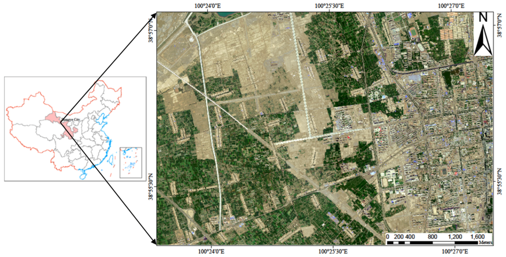
Figure 1.
Location of the study area in Zhangye City in Gansu Province, China. The image is a true color composite of the Compact Airborne Spectrographic Imager (CASI) hyperspectral image with 1 m resolution, which will be used in this study.
Figure 1.
Location of the study area in Zhangye City in Gansu Province, China. The image is a true color composite of the Compact Airborne Spectrographic Imager (CASI) hyperspectral image with 1 m resolution, which will be used in this study.

2.2. Field Measurements
Fieldwork was performed from the 10 to 17 of July 2012 across the study area to collect training samples for the supervised classification. Altogether 2086 points for the training and accuracy assessment data of supervised classification. The selection principle of the sampled points is that the identical object is required within a radius of 3 m around the sample points. The sample point coordinates were recorded by a high-accuracy Real Time Kinematic differential Global Position System (RTK dGPS) with a 1-cm survey accuracy. However, for the training samples of buildings and water bodies, we directly selected the training data from remotely sensed images because we did not determine the locations of the plot centers of buildings and water bodies with a GPS. In total, 240 buildings and 66 water bodies were selected based on a CASI image. Therefore, a total of 2392 samples were used for the land cover classification.
2.3. Remotely Sensed Data Acquisition and Processing
2.3.1. Hyperspectral Data
Airborne hyperspectral data were obtained using the Compact Airborne Spectrographic Imager (CASI-1500). The CASI-1500 sensor was on board a Harbin Y-12 aircraft on 29 June 2012. The CASI-1500 is developed by Itres Research of Canada and is a two-dimensional charge coupled device (CCD) pushbroom imager designed to acquire the visible to near infrared hyperspectral images. The CASI data have a 1 m spatial resolution covering the wavelength range from 380 nm to 1050 nm. The specific characteristics of the CASI dataset used in this study are shown in Table 1. To reduce atmospheric effects related to particulate and molecular scattering, CASI images were atmospherically corrected using the FLAASH (Fast-Line-of-sight Atmospheric Analysis of Spectral Hypercube) [45], an atmospheric correction module in the commercial software ENVI. Subsequently the hyperspectral data were orthorectified using a digital terrain model (DTM) derived from LiDAR data. To retain the original pixel values, the nearest neighbor resampling method was used [39,51]. To obtain the entire study area, CASI images were mosaicked using the mosaicking function in the ENVI software.

Table 1.
Specification of the CASI dataset used.
| Parameter | Specification |
|---|---|
| Flight height | 2000 m |
| Swath width | 1500 m |
| Number of spectral bands | 48 |
| Spatial resolution | 1.0 m |
| Spectral resolution | 7.2 nm |
| Field of view | 40° |
| Wavelength range | 380–1050 nm |
2.3.2. LiDAR Data
LiDAR point clouds were collected in July 2012 using the laser scanner of a Leica ALS70 system. The LiDAR data used were provide by the HiWATER [52]. In this study, the laser wavelength was 1064 nm with an average footprint size of 22.5 cm. The scan angle was ±18° with a 60% flight line side overlap. The average flying altitude was 1300 m. To acquire consistent point density data across the study area, we removed LiDAR point clouds in overlapping strips. After the removal of overlapping points, the average point density was 2.9 points/m2 with an average point spacing of 0.59 m, and the average point density of first echoes was 2.1 points/m2. Raw LiDAR point clouds were processed using the TerraScan software (TerraSolid, Ltd., Finland), and vegetation and ground returns were separated using the progressive triangulated irregular network (TIN) densification method proposed in the TerraScan software.
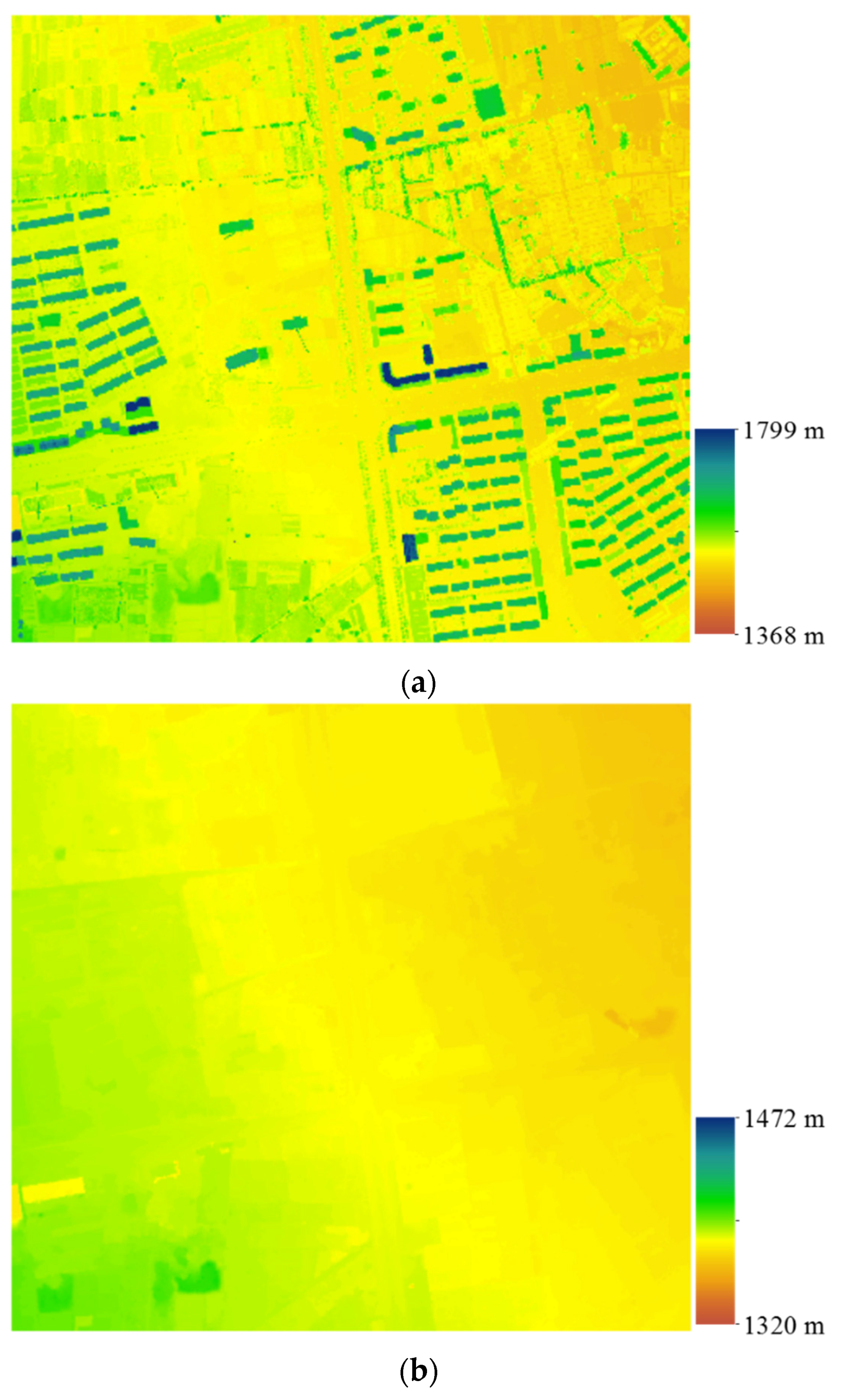
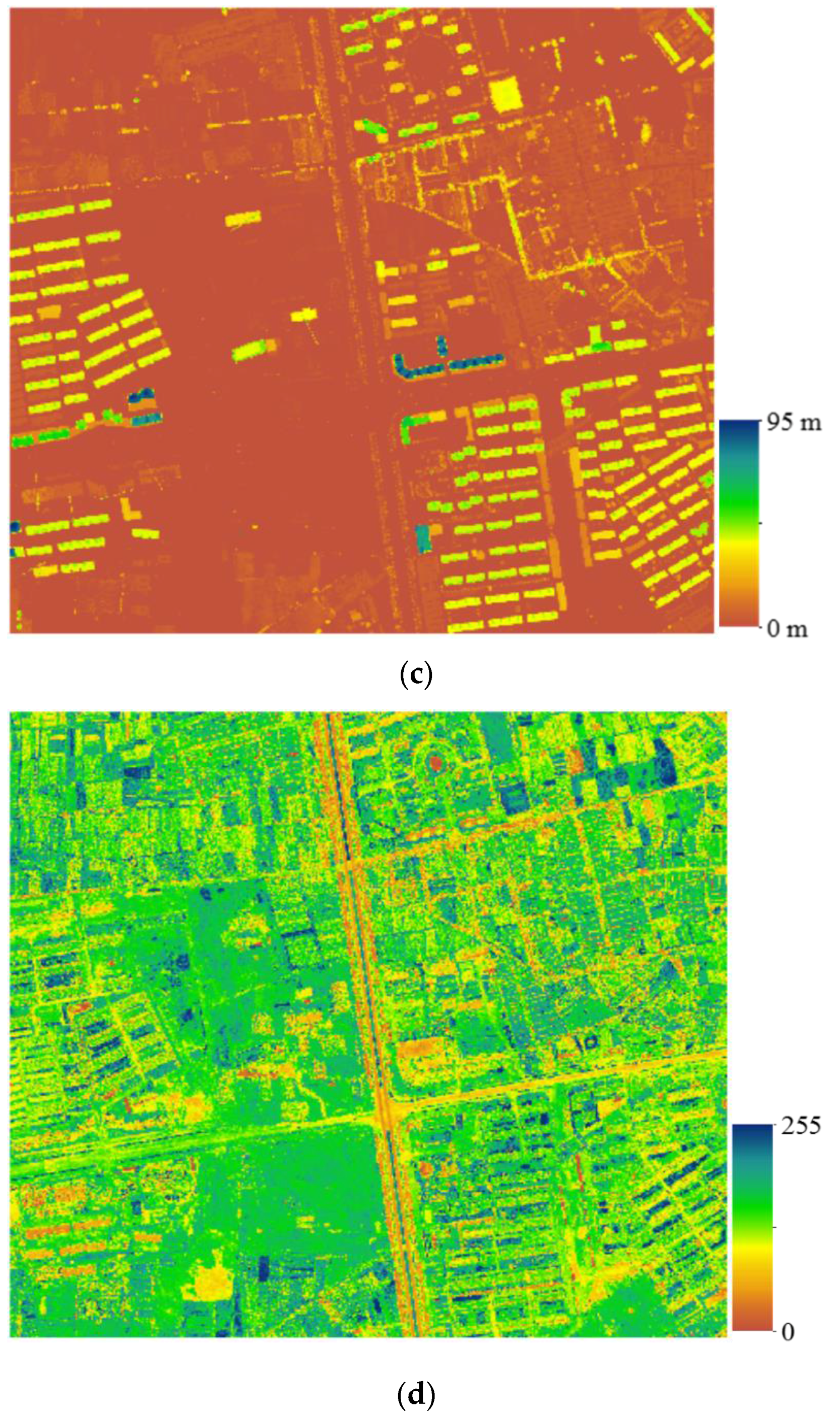
The digital surface model (DSM) (a grid size of 1.0 m) was created using the maximum height to each grid cell (Figure 2a). Empty cells were assigned elevation values by a nearest neighbor interpolation from neighboring pixels to avoid introducing new elevation values into the generated DTM [53]. The DTM was produced by computing the mean elevation value of the ground returns within each 1.0 m × 1.0 m grid cell (Figure 2b). The normalized DSM (nDSM) was then computed by subtracting the DTM from the DSM to obtain relative object height above the ground level (Figure 2c).
LiDAR intensity values are the amount of energy backscattered from features to the LiDAR sensor; these values are increasingly used [54,55,56,57]. The LiDAR intensity is closely related to laser power, incidence angle, object reflectivity and range of the LiDAR sensor to the object [43]. All these factors might cause LiDAR intensity differences for the identical type of object. Therefore, the LiDAR intensity must be corrected before they are applied to obtain a better comparison among different strips, flights and regions. Previous studies showed that normalized LiDAR intensity values can improve the accuracy of classification [58]. Consequently, to improve the classification accuracy of the land cover in our study, LiDAR intensity values were normalized by Equation (1) [59].
where Inormalized is normalized intensity, I is raw intensity, R is sensor to object distance, Rs is reference distance or average flying altitude (in this study Rs was 1300 m) and a is incidence angle.
After normalization of the LiDAR intensity, the LiDAR intensity image with a 1.0 m spatial resolution was created using the intensity field of the LiDAR points (Figure 2d). To alleviate the variation in intensity values for the identical feature, only the first echoes from the LiDAR data were used to create the intensity image [55]. When more than one laser point fell within the same pixel, the mean value of the LiDAR intensity was assigned to that pixel [60].

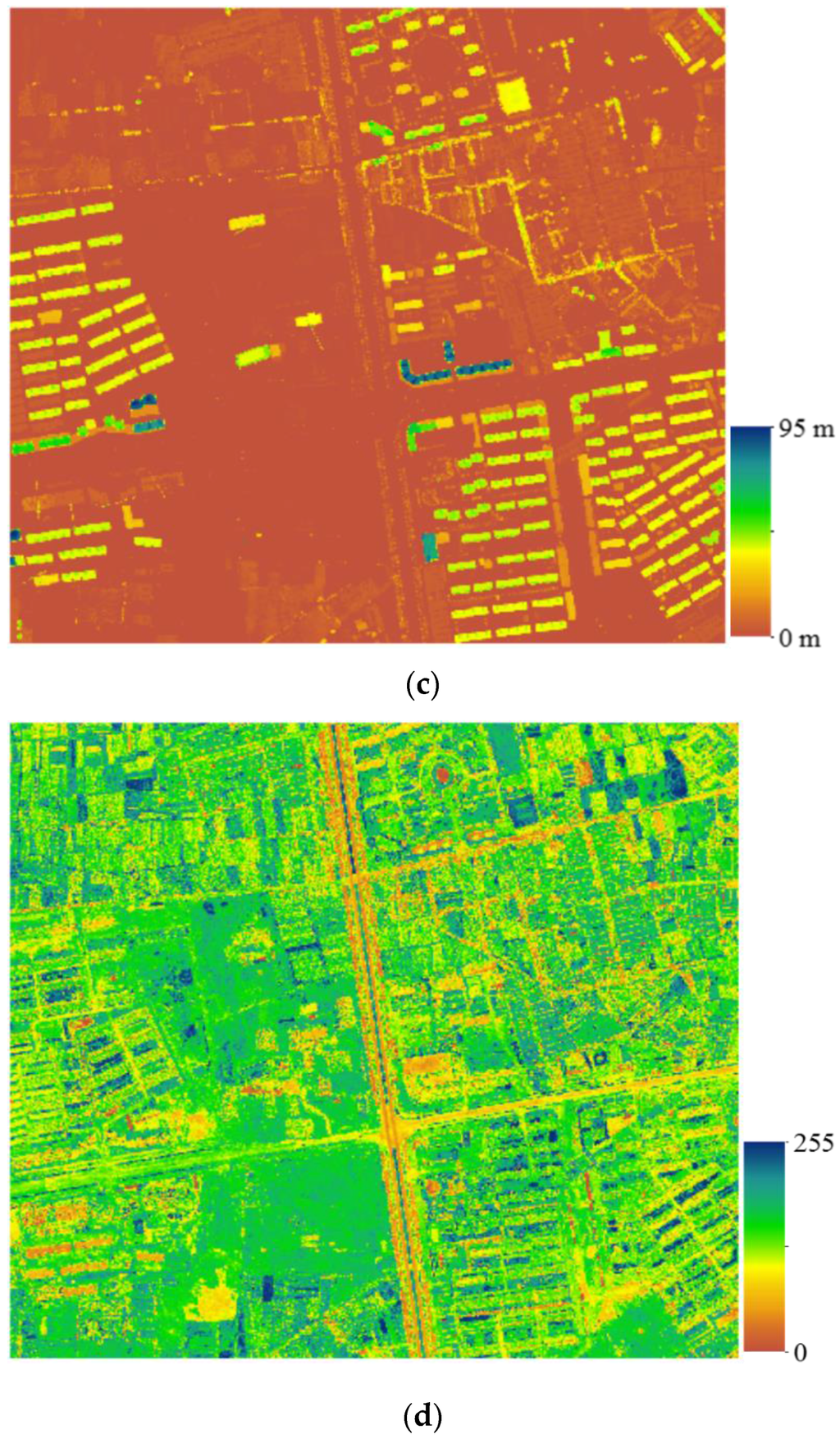
Figure 2.
Four LiDAR-derived raster images with 1 m spatial resolution: (a) digital surface model (DSM); (b) digital terrain model (DTM); (c) normalized digital surface model (nDSM); and (d) normalized LiDAR intensity image.
Figure 2.
Four LiDAR-derived raster images with 1 m spatial resolution: (a) digital surface model (DSM); (b) digital terrain model (DTM); (c) normalized digital surface model (nDSM); and (d) normalized LiDAR intensity image.
3. Methodology
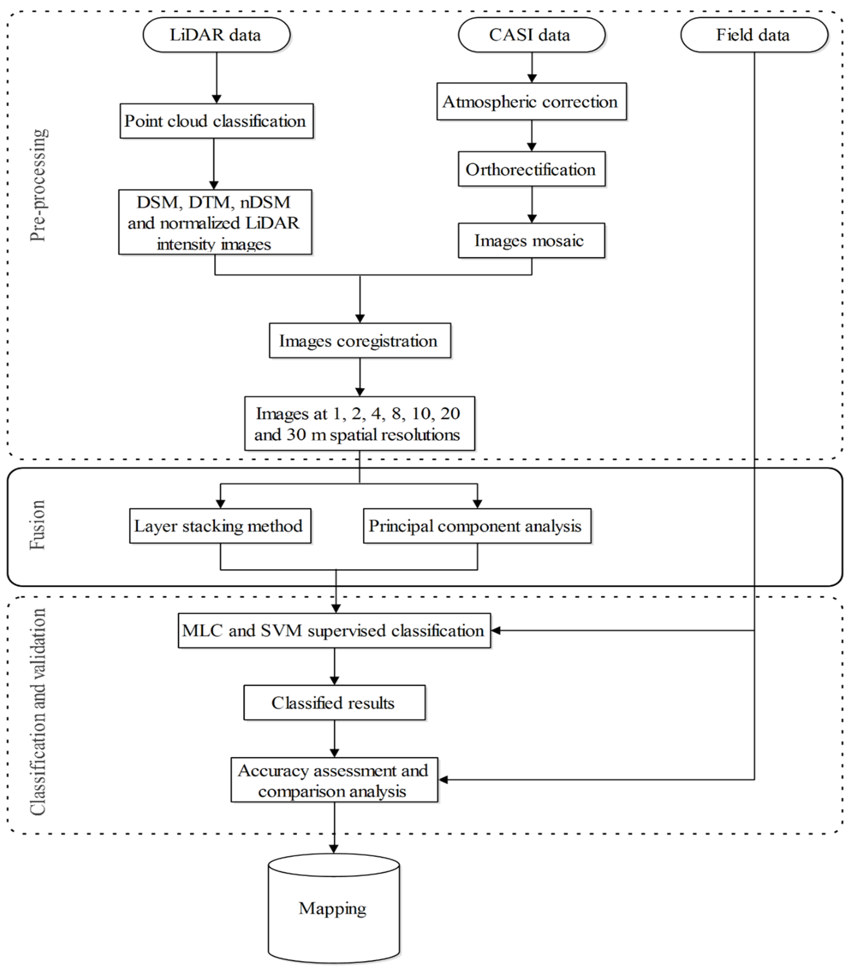
The flowchart for the data processing and land cover classification is presented in Figure 3. This figure summarizes the steps of the land cover classification using LiDAR and CASI data. Four main steps were performed including (1) pre-processing of the LiDAR and CASI data; (2) the fusion of the LiDAR and CASI data; (3) classification of the LiDAR data alone, the CASI data alone and the fused data, and (4) analyzing the classification results and assessing the accuracy. First of all, the data pre-processing was performed (see Section 2.3).

Figure 3.
Flowchart for the land cover classification using LiDAR and hyperspectral data.
Figure 3.
Flowchart for the land cover classification using LiDAR and hyperspectral data.
3.1. Fusion of the LiDAR and CASI Data
Before the data were fused, the cell values of the four LiDAR-derived raster images were linearly stretched to the 10 bit data range from 0 to 1023. In this study, the CASI data and LiDAR data were collected at different times, along with differences between the data types, flight conditions and paths produced inconsistencies in registration between the images [61]. As depicted in Figure 3a prerequisite for all fusion approaches is the accurate geometric alignment of two different data sources. Therefore, image-to-image registration of two data sources was necessary. To produce the best possible overlap between the hyperspectral CASI and LiDAR data, we coregistered the hyperspectral to the LiDAR data. The manual coregistration of these datasets was performed using the ENVI software by selecting tie points. The coregistration accuracy resulted in a root mean square error (RMSE) of less than 1 pixel (1 m).
To investigate the effect of the spatial resolution on classification accuracy, we fused LiDAR-derived images and CASI data at a range of spatial scales. Therefore, LiDAR-derived and CASI data with 1 m spatial resolution were spatially resampled to 2, 4, 8, 10, 20 and 30 m resolutions using a nearest neighbor resampling method before data fusion.
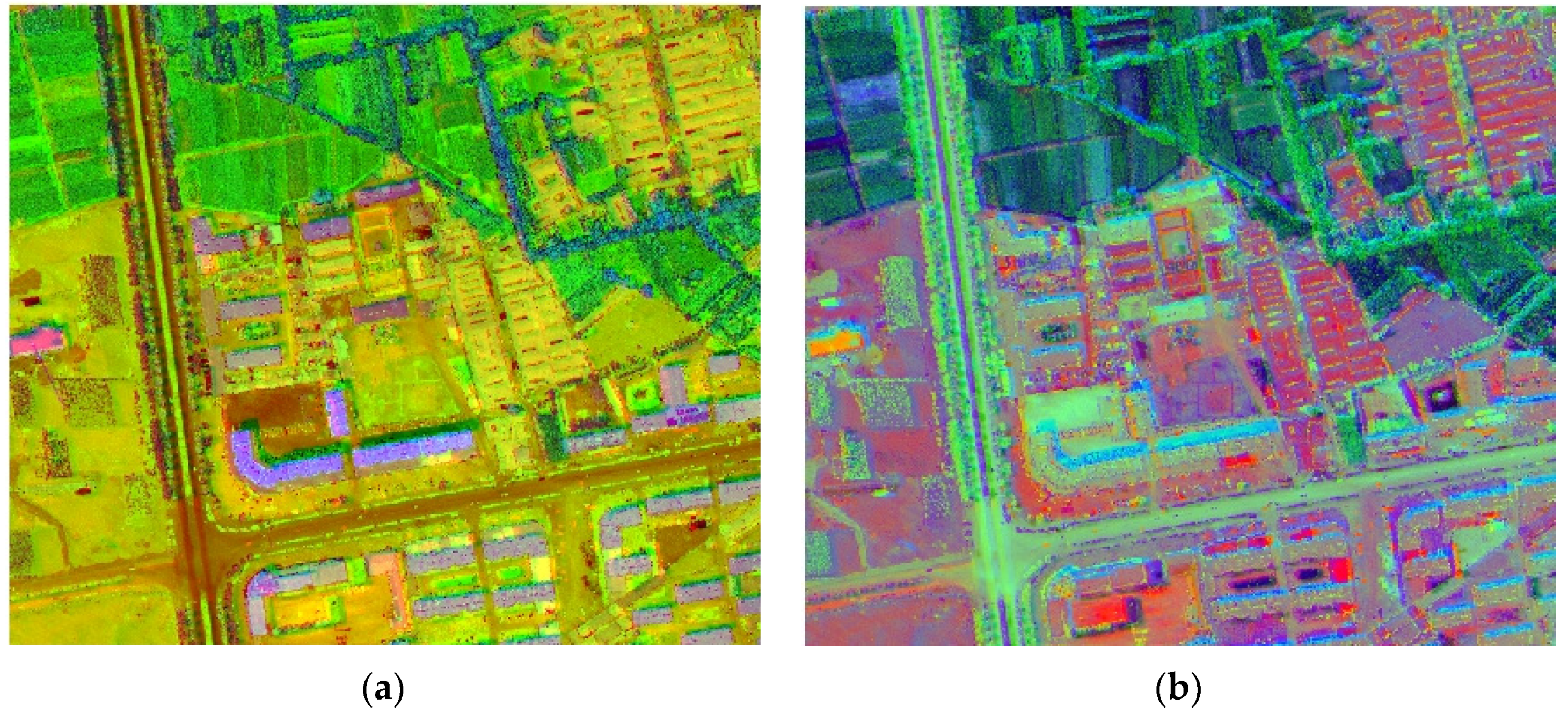
Data fusion is the integration of two or more different datasets to form a new data utilizing a certain algorithm. It can be implemented at different levels: at the decision level, feature level, and pixel level [62]. The goal of data fusion is to integrate complementary data to acquire high quality data with more abundant information. This process has been extensively used in the field of remote sensing [63]. Data fusion of LiDAR and other remote sensing data is a critical part of this study. The selection of data fusion methods between LiDAR and CASI data could have an influence on the land cover classification results. Therefore, to obtain the best fusion method for different data sources and applications, a trial and error method is necessary. In this study, to obtain the optimal fusion method of LiDAR and CASI data for land classification, both layer stacking and principal component analysis (PCA) fusion methods were tested. PCA is an orthogonal linear transformation, which transforms the data to a new coordinate system to reduce the multidimensional datasets into lower dimensions [64]. PCA transformations will produce some uncorrelated variables called principal components, and only the first few principal components may account for meaningful amounts of variance in the original data [65]. We used the layer stacking method to combine four LiDAR-derived images (DTM, DSM, nDSM, and intensity) and CASI data (48 bands) into one multiband image at the pixel level. This new multiband image includes a total of 52 bands. Figure 4a shows the 3 band image (near infrared image of CASI, the intensity image and nDSM) of the LiDAR-CASI stacked image with 52 bands. For the stacked image, we used two methods to process the image. The first method was directly classifying the stacked image with 52 bands. The second method was transforming the stacked image using a PCA algorithm, and then the first few principal components derived from the PCA were used as the data for the land cover classification. The PCA transformation could reduce data redundancy and retain the uncorrelated variables (i.e., independent principal components). In this study, we found that the first five principal components account for 98.93% of the total variance in the whole LiDAR and CASI data. Therefore, the first five principal components were used to replace the stacked image (52 bands), and the redundancy, noise, and size of the dataset were significantly reduced [44]. Figure 4b illustrates the image of the first three principal components image in the principal component analysis of the LiDAR-CASI stacked image with 52 bands.
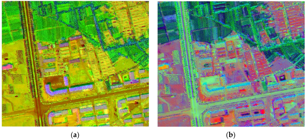
Figure 4.
LiDAR-CASI fusion images with 1 m spatial resolution: (a) LiDAR-CASI stacked image (near infrared image of CASI, intensity image and nDSM); and (b) principal component analysis (first three principal components).
Figure 4.
LiDAR-CASI fusion images with 1 m spatial resolution: (a) LiDAR-CASI stacked image (near infrared image of CASI, intensity image and nDSM); and (b) principal component analysis (first three principal components).
3.2. Classification Methods
Generally, remote sensing classification methods are divided into two broad types: parametric and non-parametric methods [66]. Parametric methods are based on the assumption that the data of each class are normally distributed [7,49,67]; however, non-parametric techniques do not assume specific data class distributions [11,41]. Supervised classification is one of the most commonly used techniques for the classification of remotely sensed data. In this study, two supervised classification methods were performed: (1) maximum likelihood classification (MLC) method; (2) support vector machine (SVM) classification.
The MLC method is a simple, yet robust, classifier [39,51]. The MLC is a parametric classifier based on the Bayesian decision theory and is the most popular conventional supervised classification technique [68,69]. However, for the MLC method, it is difficult to satisfy the assumption of a normally distributed dataset. Another disadvantage of conventional parametric classification approaches is that they are limited in their ability to classify multisource and high dimensional data [67]. However, the SVM classifier is a non-parametric classifier for supervised classification [45,70], which is able to handle non-normal distributed datasets [11,30]. The primary advantage of the SVM method is that it requires no assumptions in terms of the distribution of the data and can achieve a good result with relatively limited training sample data [5,67]. In addition, the SVM method is not sensitive to high data dimensionality [11,41,71], and is especially suited to classify data with high dimensionality and multiple sources [9,67]. In general, previous studies have shown that the SVM is more accurate than the MLC method, e.g., [66,72]. To validate the better performance of the SVM classifier compared with other parametric approaches in our study, the MLC was performed and the results were compared with those produced from the SVM classifier.
In this study, we performed a land cover classification at seven different spatial scales (1, 2, 4, 8, 10, 20 and 30 m) to determine an optimal spatial scale for the classification using different datasets. In addition, to compare the classification accuracies of the fusion data with those of a single data source, single source LiDAR and CASI data were also classified. Therefore, four different remotely sensed datasets were trained: (a) LiDAR-derived images alone; (b) the CASI images alone (48 bands); (c) the layer stacking image with 52 bands (CASI: 48 bands, LiDAR: four images); and (d) the first five principal components derived from the PCA transformation. Finally, twenty-eight datasets were classified using the MLC and SVM supervised classifiers.
The land cover category was classified into seven classes, i.e., buildings, road, water bodies, forests, grassland, cropland and barren land. For each land cover category, about two-thirds of the samples were randomly selected as training data, with the remaining samples used to assess the classification accuracies. Table 2 lists the per-class numbers for the classification training and validation data (a total of 2392 samples).
Table 2.
The number of classification training and validation data per class.
| Class | Number of Training Sample (Points) | Number of Validation Sample (Points) |
|---|---|---|
| Buildings | 160 | 80 |
| Road | 225 | 113 |
| Water bodies | 44 | 22 |
| Forests | 397 | 198 |
| Grassland | 278 | 139 |
| Cropland | 307 | 154 |
| Barren land | 183 | 92 |
| 1594 | 798 |
3.3. Accuracy Assessment
The number of validation samples per class based on separate test data is shown in Table 2. A total of 798 samples were applied to assess the classification accuracies. Classification accuracies were assessed based on confusion matrices (also called the error matrixes), which is the most standard method for remote sensing classification accuracy assessments [72]. The accuracy metrics include the overall accuracy (OA), the producer’s accuracy (PA), the error of omission (i.e., 1-PA), the user’s accuracy (UA), the error of commission (i.e., 1-UA) and the kappa coefficient (K). These accuracy metrics can be acquired from the confusion matrixes; these matrixes are widely used in classification accuracy assessment of remote sensing [13]. We assessed and compared the classification accuracies of 56 classification maps produced by the MLC and SVM classifiers.
4. Results and Discussion
Supervised classifications were performed on four datasets with seven different spatial resolutions using the MLC and SVM classifiers. Each classifier produced 28 classification results, and a total of 56 classification results were obtained. The classification accuracies were evaluated using one-third of the samples collected which were not used in the supervised classification. The classification accuracies of the 56 classification maps produced by the MLC and SVM classifiers are shown in Table 3.
Table 3.
Classification accuracies of the maximum likelihood classification (MLC) and support vector machine (SVM) classifiers using four types of datasets with different spatial resolutions. The accuracy metrics included the overall accuracy (OA) and kappa coefficient (K).
| Resolution (meters) | Accuracy Metrics | LiDAR and CASI Data Alone | Fused Data of LiDAR and CASI | |||||||||
|---|---|---|---|---|---|---|---|---|---|---|---|---|
| LiDAR Data | CASI Data | PCA | Layer stacking | |||||||||
| MLC | SVM | MLC | SVM | MLC | SVM | MLC | SVM | |||||
| 1 | OA (%) | 25 | 75.6 | 84.7 | 88.7 | 91.9 | 95.3 | 92.9 | 97.8 | |||
| K | 0.181 | 0.582 | 0.758 | 0.836 | 0.868 | 0.923 | 0.888 | 0.964 | ||||
| 2 | OA (%) | 27.8 | 78.2 | 82.8 | 87.1 | 90.7 | 96.5 | 92.1 | 97.7 | |||
| K | 0.203 | 0.654 | 0.743 | 0.825 | 0.862 | 0.943 | 0.884 | 0.963 | ||||
| 4 | OA (%) | 34.1 | 74.5 | 80.2 | 85.6 | 89.9 | 94.5 | 91.2 | 96.3 | |||
| K | 0.262 | 0.626 | 0.726 | 0.803 | 0.86 | 0.922 | 0.878 | 0.948 | ||||
| 8 | OA (%) | 37.8 | 69.5 | 76.6 | 81.1 | 87.1 | 88.9 | 89 | 92.8 | |||
| K | 0.292 | 0.579 | 0.694 | 0.757 | 0.829 | 0.849 | 0.855 | 0.904 | ||||
| 10 | OA (%) | 39.3 | 68.2 | 75.6 | 80.5 | 85.9 | 87.9 | 87.7 | 91.2 | |||
| K | 0.302 | 0.561 | 0.692 | 0.746 | 0.814 | 0.836 | 0.84 | 0.883 | ||||
| 20 | OA (%) | 53.5 | 62.6 | 74.8 | 77.3 | 81.5 | 81.2 | 84.5 | 86.5 | |||
| K | 0.401 | 0.445 | 0.679 | 0.692 | 0.741 | 0.723 | 0.783 | 0.805 | ||||
| 30 | OA (%) | 48.7 | 60.3 | 73.1 | 71.2 | 81.4 | 79.7 | 83.3 | 82 | |||
| K | 0.298 | 0.401 | 0.619 | 0.589 | 0.696 | 0.644 | 0.727 | 0.686 | ||||
| Mean | OA (%) | 38 | 69.8 | 78.3 | 81.6 | 86.9 | 89.1 | 88.7 | 92 | |||
| K | 0.277 | 0.55 | 0.702 | 0.75 | 0.81 | 0.834 | 0.836 | 0.879 | ||||
4.1. Comparison of Classification Results with Different Datasets
Data fusion has been extensively used in the remote sensing field. Data fusion can implement data compression, image enhancement and complementary information for multiple data sources. To determine the performance of different fused methods for land cover classification, the PCA and the layer stacking were applied to fuse LiDAR and CASI data. For the four types of datasets (i.e., LiDAR data, CASI data, PCA data and layer stacking images), the LiDAR data alone produced the worst classification result; the lowest overall classification accuracy (OA = 25.0%, K = 0.181) was produced using the MLC classifier at 1 m resolution, and the highest accuracy was only 78.2% with a kappa of 0.654 at 2 m spatial resolution. This poor classification accuracy could be explained by the lack spectral information in LiDAR data, which could provide useful information related to land cover. Therefore, it was difficult to obtain accurate land cover classification using only LiDAR data. The layer stacking fusion data obtained the best classification result, and the highest accuracy was 97.8% with a kappa of 0.964 at 1 m spatial resolution. The highest overall classification accuracies for the PCA fused data and CASI data alone were 96.5% and 88.7%, respectively. The results showed that the overall classification accuracies of LiDAR and CASI fusion data outperformed the LiDAR and CASI data alone (Table 3). This result was consistent with findings reported by Singh, et al. [39]. The increased accuracies could be attributed to complementary vertical and spectral information from the LiDAR and CASI data.

Figure 5.
Improvements in the land cover classification accuracies for the layer stacking data compared with three other datasets (PCA, CASI and LiDAR) using the SVM and MLC classifiers at seven spatial resolutions; (a) overall accuracy and (b) kappa coefficient.
Figure 5.
Improvements in the land cover classification accuracies for the layer stacking data compared with three other datasets (PCA, CASI and LiDAR) using the SVM and MLC classifiers at seven spatial resolutions; (a) overall accuracy and (b) kappa coefficient.
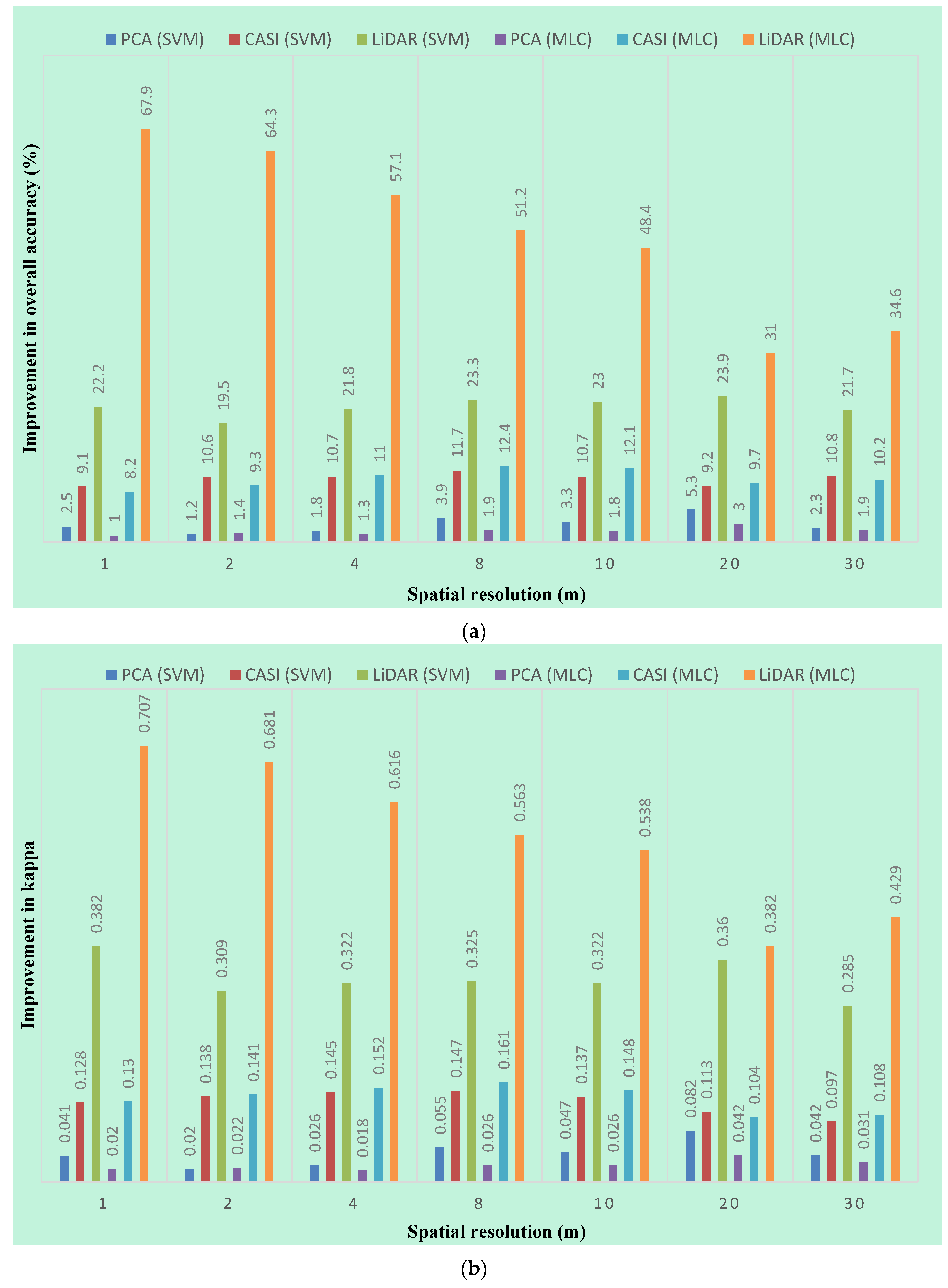
For the fused data, all overall classification accuracies for the seven spatial resolutions were greater than or equal to 79.7%. Moreover, the overall accuracies of fusion datasets exceeded 94% using the SVM classifier at the 1 m, 2 m and 4 m spatial resolutions. In our study, the overall classification accuracies of the CASI and LiDAR fusion data were 9.1% and 19.6% higher than the CASI and LiDAR data alone, respectively. Previous study has shown that different data fusion methods have an effect on the land cover classification accuracies [44]. In this study, we obtained similar results. Table 3 demonstrates that the stacking fusion data produced higher overall accuracies and kappa coefficients using both SVM and MLC classifiers than that of PCA fusion data. The average overall classification accuracies of the layer stacking fusion data based on the SVM and MLC classifier were 2.90% and 1.76% higher than that of the PCA fusion data, respectively. Figure 5 shows the improvements in the classification accuracies for the layer stacking data compared with three other datasets (PCA, CASI and LiDAR) using the SVM and MLC classifiers at seven spatial resolutions. In short, the fused data of LiDAR and CASI improved the classification accuracy, and we found that the layer stacking fusion method generally performed better than the PCA fusion method for land cover classification. However, these results do not indicate that the layer stacking method always performs better than the PCA method in all cases.
4.2. Classification Performance of the MLC and SVM Classifiers
Figure 6 illustrates the comparison of the classification results produced from the MLC and SVM classifiers with all four datasets at seven spatial resolutions. For the stacked image, the average overall accuracies for the SVM and MLC classifiers at all seven spatial resolutions were 92% and 88.7%, respectively. Comparison of the highest classification accuracies produced from the SVM and MLC classifier showed that the SVM classifier obtained a slightly higher accuracy, improving the overall accuracy of approximately 4.9%. The result indicated that the distribution-free SVM classifier generally performed better than the MLC classifier. This result was consistent with the findings presented by García et al. [67], who found that the SVM classifier could improve the overall accuracy of land cover classification. Therefore, the SVM is more suitable for a high dimensionality and multiple sources dataset than the parametric methods commonly used in remotely sensed image supervised classification [9,41]. However, the disadvantage of the SVM classifier is that it increases computational demands compared with the MLC classifier [73]. Consequently, the SVM classifier may be time consuming when classifying the land cover of a large data volume. We must acquire a good balance between the accuracy and efficiency of the classification according to the purposes and requirements of the work.
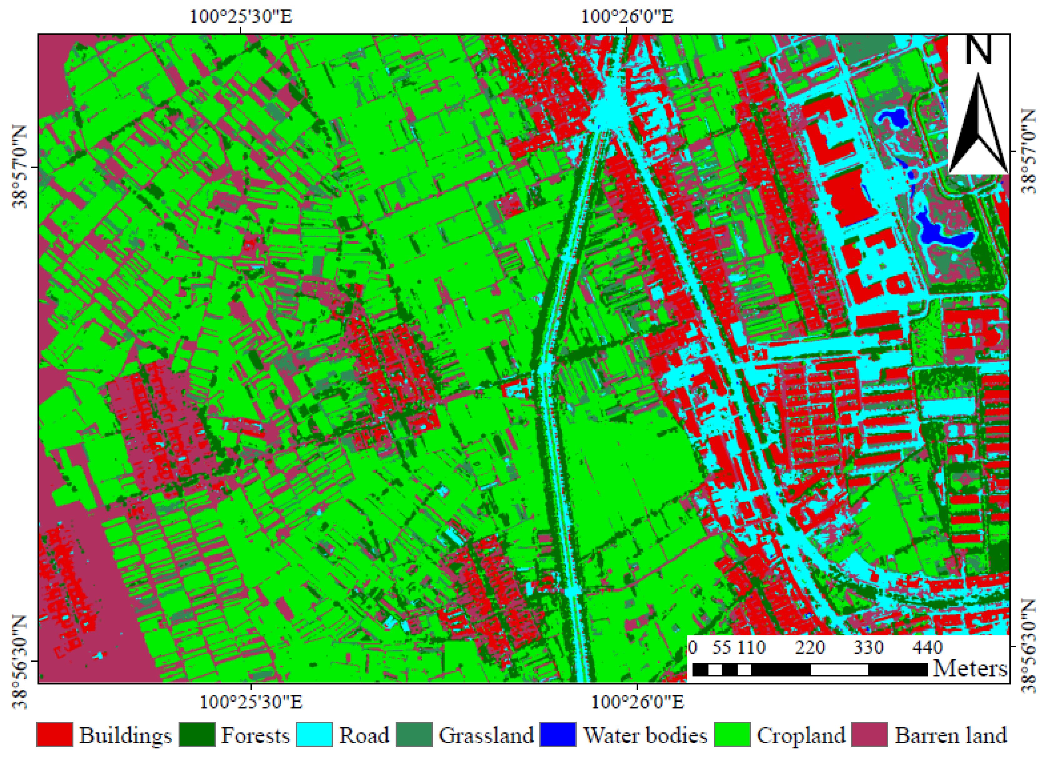
Table 4 shows the accuracy of each class from the confusion matrices of the highest overall classification accuracy produced by the SVM and MLC classifiers for layer stacking fusion data at 1 m spatial resolution. The results showed that the SVM classifier generally obtained higher user’s accuracy and producer’s accuracy than the MLC classifier. For the SVM classifier, the user’s accuracies and producer’s accuracies of all seven classes (i.e., buildings, road, water bodies, forests, grassland, cropland and barren land) exceed 80.1% and 84.5%, respectively. Although the overall accuracy of the MLC classifier was relatively high (OA = 92.9%, kappa = 0.888), the two largest errors of commission were observed for forests (63.67%) and grassland (43.99%), and the two largest errors of omission were road (29.85%) and forests (18.05%). Correspondingly, low errors were obtained using the SVM classification method, and the errors of commission were 1.93% (forests) and 19.87% (grassland), and the errors of omission were 8.85% (road) and 15.47% (forests). In general, compared with the MLC classifier, the SVM improved the user’s accuracies of forests and grassland and producer’s accuracies of road and forests in this study. Therefore, we produced a land cover classification map of the study area using the SVM classifier, obtaining the highest overall accuracy using the layer stacking fusion data at a 1 m spatial resolution. Following the supervised classification, a post-classification process based on a majority filter was used to remove isolated pixels [68]. Figure 7 is the subset of the study area classification map with an overall accuracy of 97.8% (kappa = 0.964).
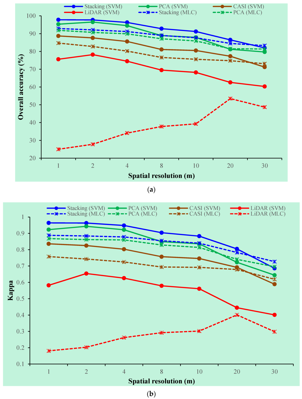
Figure 6.
Comparison of the classification accuracies using different classifiers, datasets and spatial resolutions; (a) overall accuracy and (b) kappa coefficient.
Figure 6.
Comparison of the classification accuracies using different classifiers, datasets and spatial resolutions; (a) overall accuracy and (b) kappa coefficient.

Table 4.
Per-class accuracies obtained with the highest overall accuracy produced by the support vector machine (SVM) and maximum likelihood (MLC) classifiers for layer stacking fusion data at a 1 m spatial resolution. The accuracies included the producer’s accuracy (PA), user’s accuracy (UA), error of commission (EC) and error of omission (EO).
| Class Name | SVM Classifier | MLC Classifier | |||||||
|---|---|---|---|---|---|---|---|---|---|
| PA (%) | UA(%) | EO (%) | EC (%) | PA (%) | UA (%) | EO (%) | EC (%) | ||
| Buildings | 94.78 | 99.58 | 5.22 | 0.42 | 94.73 | 97.85 | 5.27 | 2.15 | |
| Road | 91.15 | 94.58 | 8.85 | 5.42 | 70.15 | 88.42 | 29.85 | 11.58 | |
| Water bodies | 99.99 | 99.92 | 0.01 | 0.08 | 96.05 | 100 | 3.95 | 0 | |
| Forests | 84.53 | 98.07 | 15.47 | 1.93 | 81.95 | 36.33 | 18.05 | 63.67 | |
| Grassland | 93.44 | 80.13 | 6.56 | 19.87 | 89.55 | 56.01 | 10.45 | 43.99 | |
| Cropland | 99.8 | 95.42 | 0.2 | 4.58 | 99.53 | 94.2 | 0.47 | 5.8 | |
| Barren land | 94.7 | 94.48 | 5.3 | 5.52 | 89.76 | 99.4 | 10.24 | 0.6 | |
| OA (%) | 97.8 | 92.9 | |||||||
| K | 0.964 | 0.888 | |||||||

Figure 7.
Land cover classification map using the SVM classifier based on the layer stacking fusion method at a 1 m spatial resolution (OA = 97.8%, kappa = 0.964).
Figure 7.
Land cover classification map using the SVM classifier based on the layer stacking fusion method at a 1 m spatial resolution (OA = 97.8%, kappa = 0.964).
For the layer stacking fusion data and CASI data alone at a 30 m spatial resolution, the MLC classifier obtained better results (OA = 83.3% and 73.1%, respectively) than that of the SVM classifier (OA = 82% and 71.2%, respectively). For the PCA fusion data, the overall classification accuracies of the MLC classifier both at 20 m and 30 m were higher than that of the SVM classifier. Therefore, the SVM classifier was not always the optimal classifier at all seven resolutions. This result was consistent with the results observed by Ghosh, et al. [48], who claimed that none of the classifiers produced consistently higher accuracies at all spatial resolutions. For the LiDAR data alone, the SVM classifier displayed higher accuracies than the MLC classifiers at all seven spatial resolutions. In general, our results demonstrated that the classification accuracies were affected by the dataset types, spatial resolutions and classifiers.
4.3. Influence of the Spatial Resolution on the Classification Accuracy
Spatial resolution of remotely sensed data is one of the most critical factors that affects the classification accuracies [74]. In this study, therefore, the land cover was classified at seven spatial scales (1, 2, 4, 8, 10, 20 and 30 m) to obtain an optimal spatial resolution for the classification with four types of datasets. We analyzed the optimal resolutions for each datasets and classifier. Different optimal resolutions were found for the four datasets and two classification methods, and similar results were also presented by Ke, et al. [74]. For the PCA and LiDAR data using the SVM classifier, the highest classification accuracies were obtained at a 2 m spatial resolution (Figure 6). After that, the overall classification accuracy started to decrease. However, for the LiDAR data using the MLC classifier, the classification accuracies increased as spatial resolutions became coarser (from 1 m to 20 m), and the overall accuracy was the highest at a 20 m spatial resolution. Except for the above-mentioned results, the classification results showed that classification accuracy generally decreased as spatial resolution of the input datasets became coarser, and the highest classification accuracies were found at a 1 m spatial resolution (Figure 6). Therefore, the higher classification accuracy does not always occur for the higher spatial resolutions in the different datasets. In addition, although the classification accuracy is high for select datasets with a fine resolution, a substantial amount of data covers large areas for land cover classification. Thus, data management and processing will become a problem, and the classification performance will decrease. In conclusion, when classifying land cover, we should select the optimal spatial resolution based on the application and research purposes.
5. Conclusions
This study explored the potential for fusing airborne LiDAR and hyperspectral CASI data to classify land cover. We fused LiDAR and CASI data using layer stacking and PCA fusion methods, and successfully performed supervised image classification using the SVM and MLC classifiers. Overall, the use of fused data between LiDAR and CASI for land cover classification outperformed the classification accuracies produced from LiDAR and CASI data alone (Table 3). The highest overall accuracy (OA = 97.8% with a kappa of 0.964) was generated by the non-parametric SVM classifier when using layer stacking fusion data at 1 m spatial resolution. Compared with the best classification results of the CASI and LiDAR data alone, the overall classification accuracies improved by 9.1% and 19.6%, respectively. Moreover, we found that the classification accuracies based on the layer stacking data were higher than that based on a PCA for all spatial resolutions. In this study, therefore, the layer stacking fusion method was more suitable for the land cover classification compared to the PCA fusion method. Using the SVM classifier to classify the fused LiDAR and CASI data produced a higher accuracy than that of the MLC classifier. This result showed that the SVM classifier possesses a higher potential than the MLC for land cover classification using multisource fusion data from LiDAR and CASI data.
LiDAR and multi/hyperspectral remote sensing fusion data have provided complementary information that LiDAR and multi/hyperspectral data alone have not. Therefore, the fusion of LiDAR and multi/hyperspectral data has a great potential for highly accurate information extraction of objects and land cover mapping. Our future work will focus on fusing LiDAR and passive optical remotely sensed data to classify different vegetation types and land covers to estimate the vegetation biomass and to detect land cover changes.
Acknowledgments
This work was supported by the National Natural Science Foundation of China (Nos. 41371350 and 41271428); the International Postdoctoral Exchange Fellowship Program 2014 by the Office of China Postdoctoral Council (20140042); Beijing Natural Science Foundation (4144074). We are grateful to the four anonymous reviewers and associate editor Danielle Yao for their valuable comments and suggestions on the manuscript.
Author Contributions
Shezhou Luo and Cheng Wang contributed the main idea, designed the study method, and finished the manuscript. Xiaohuan Xi and Hongcheng Zeng processed LiDAR data. Dong Li, Shaobo Xia and Pinghua Wang processed CASI data. The manuscript was improved by the contributions of all of the co-authors.
Conflicts of Interest
The authors declare no conflict of interest.
References
- Foody, G.M. Assessing the accuracy of land cover change with imperfect ground reference data. Remote Sens. Environ. 2010, 114, 2271–2285. [Google Scholar] [CrossRef]
- Turner, B.L.; Lambin, E.F.; Reenberg, A. The emergence of land change science for global environmental change and sustainability. Proc. Natl. Acad. Sci. USA 2007, 104, 20666–20671. [Google Scholar] [CrossRef] [PubMed]
- Gong, P.; Wang, J.; Yu, L.; Zhao, Y.; Zhao, Y.; Liang, L.; Niu, Z.; Huang, X.; Fu, H.; Liu, S.; et al. Finer resolution observation and monitoring of global land cover: First mapping results with Landsat TM and ETM+ data. Int. J. Remote Sens. 2012, 34, 2607–2654. [Google Scholar] [CrossRef]
- Liu, Y.; Zhang, B.; Wang, L.-M.; Wang, N. A self-trained semisupervised svm approach to the remote sensing land cover classification. Comput. Geosci. 2013, 59, 98–107. [Google Scholar] [CrossRef]
- Fieber, K.D.; Davenport, I.J.; Ferryman, J.M.; Gurney, R.J.; Walker, J.P.; Hacker, J.M. Analysis of full-waveform LiDAR data for classification of an orange orchard scene. ISPRS J. Photogramm. Remote Sens. 2013, 82, 63–82. [Google Scholar] [CrossRef]
- Chasmer, L.; Hopkinson, C.; Veness, T.; Quinton, W.; Baltzer, J. A decision-tree classification for low-lying complex land cover types within the zone of discontinuous permafrost. Remote Sens. Environ. 2014, 143, 73–84. [Google Scholar] [CrossRef]
- Pal, M.; Mather, P.M. Assessment of the effectiveness of support vector machines for hyperspectral data. Future Gener. Comput. Syst. 2004, 20, 1215–1225. [Google Scholar] [CrossRef]
- Szuster, B.W.; Chen, Q.; Borger, M. A comparison of classification techniques to support land cover and land use analysis in tropical coastal zones. Appl. Geogr. 2011, 31, 525–532. [Google Scholar] [CrossRef]
- Waske, B.; Benediktsson, J.A. Fusion of support vector machines for classification of multisensor data. IEEE Trans. Geosci. Remote Sens. 2007, 45, 3858–3866. [Google Scholar] [CrossRef]
- Berger, C.; Voltersen, M.; Hese, O.; Walde, I.; Schmullius, C. Robust extraction of urban land cover information from HSR multi-spectral and LiDAR data. IEEE J. Sel. Topics Appl. Earth Obs. Remote Sens. 2013, 6, 2196–2211. [Google Scholar] [CrossRef]
- Klein, I.; Gessner, U.; Kuenzer, C. Regional land cover mapping and change detection in central asia using MODIS time-series. Appl. Geogr. 2012, 35, 219–234. [Google Scholar] [CrossRef]
- Adam, E.; Mutanga, O.; Odindi, J.; Abdel-Rahman, E.M. Land-use/cover classification in a heterogeneous coastal landscape using Rapideye imagery: Evaluating the performance of random forest and support vector machines classifiers. Int. J. Remote Sens. 2014, 3440–3458. [Google Scholar] [CrossRef]
- Puertas, O.L.; Brenning, A.; Meza, F.J. Balancing misclassification errors of land cover classification maps using support vector machines and Landsat imagery in the Maipo River Basin (Central Chile, 1975–2010). Remote Sens. Environ. 2013, 137, 112–123. [Google Scholar] [CrossRef]
- Lu, D.; Chen, Q.; Wang, G.; Moran, E.; Batistella, M.; Zhang, M.; Vaglio Laurin, G.; Saah, D. Aboveground forest biomass estimation with Landsat and LiDAR data and uncertainty analysis of the estimates. Int. J. For. Res. 2012, 2012, 1–16. [Google Scholar] [CrossRef]
- Edenius, L.; Vencatasawmy, C.P.; Sandström, P.; Dahlberg, U. Combining satellite imagery and ancillary data to map snowbed vegetation important to Reindeer rangifer tarandus. Arct. Antarct. Alp. Res. 2003, 35, 150–157. [Google Scholar] [CrossRef]
- Amarsaikhan, D.; Blotevogel, H.H.; van Genderen, J.L.; Ganzorig, M.; Gantuya, R.; Nergui, B. Fusing high-resolution sar and optical imagery for improved urban land cover study and classification. Int. J. Image Data Fusion 2010, 1, 83–97. [Google Scholar] [CrossRef]
- Dong, P. LiDAR data for characterizing linear and planar geomorphic markers in tectonic geomorphology. J. Geophys. Remote Sens. 2015. [Google Scholar] [CrossRef]
- Richardson, J.J.; Moskal, L.M.; Kim, S.-H. Modeling approaches to estimate effective leaf area index from aerial discrete-return LiDAR. Agric. For. Meteorol. 2009, 149, 1152–1160. [Google Scholar] [CrossRef]
- Lee, H.; Slatton, K.C.; Roth, B.E.; Cropper, W.P. Prediction of forest canopy light interception using three-dimensional airborne LiDAR data. Int. J. Remote Sens. 2009, 30, 189–207. [Google Scholar] [CrossRef]
- Brennan, R.; Webster, T.L. Object-oriented land cover classification of LiDAR-derived surfaces. Can. J. Remote Sens. 2006, 32, 162–172. [Google Scholar] [CrossRef]
- Ko, C.; Sohn, G.; Remmel, T.; Miller, J. Hybrid ensemble classification of tree genera using airborne LiDAR data. Remote Sens. 2014, 6, 11225–11243. [Google Scholar] [CrossRef]
- Luo, S.; Wang, C.; Pan, F.; Xi, X.; Li, G.; Nie, S.; Xia, S. Estimation of wetland vegetation height and leaf area index using airborne laser scanning data. Ecol. Indicators 2015, 48, 550–559. [Google Scholar] [CrossRef]
- Tang, H.; Brolly, M.; Zhao, F.; Strahler, A.H.; Schaaf, C.L.; Ganguly, S.; Zhang, G.; Dubayah, R. Deriving and validating leaf area index (LAI) at multiple spatial scales through LiDAR remote sensing: A case study in Sierra National Forest. Remote Sens. Environ. 2014, 143, 131–141. [Google Scholar] [CrossRef]
- Hopkinson, C.; Chasmer, L. Testing LiDAR models of fractional cover across multiple forest EcoZones. Remote Sens. Environ. 2009, 113, 275–288. [Google Scholar] [CrossRef]
- Glenn, N.F.; Spaete, L.P.; Sankey, T.T.; Derryberry, D.R.; Hardegree, S.P.; Mitchell, J.J. Errors in LiDAR-derived shrub height and crown area on sloped terrain. J. Arid Environ. 2011, 75, 377–382. [Google Scholar] [CrossRef]
- Zhao, K.; Popescu, S.; Nelson, R. LiDAR remote sensing of forest biomass: A scale-invariant estimation approach using airborne lasers. Remote Sens. Environ. 2009, 113, 182–196. [Google Scholar] [CrossRef]
- Antonarakis, A.S.; Richards, K.S.; Brasington, J. Object-based land cover classification using airborne LiDAR. Remote Sens. Environ. 2008, 112, 2988–2998. [Google Scholar] [CrossRef]
- Qin, Y.; Li, S.; Vu, T.-T.; Niu, Z.; Ban, Y. Synergistic application of geometric and radiometric features of LiDAR data for urban land cover mapping. Opt. Express 2015, 23, 13761–13775. [Google Scholar] [CrossRef] [PubMed]
- Sherba, J.; Blesius, L.; Davis, J. Object-based classification of abandoned logging roads under heavy canopy using LiDAR. Remote Sens. 2014, 6, 4043–4060. [Google Scholar] [CrossRef]
- Mallet, C.; Bretar, F.; Roux, M.; Soergel, U.; Heipke, C. Relevance assessment of full-waveform LiDAR data for urban area classification. ISPRS J. Photogramm. Remote Sens. 2011, 66, S71–S84. [Google Scholar] [CrossRef]
- Hellesen, T.; Matikainen, L. An object-based approach for mapping shrub and tree cover on grassland habitats by use of LiDAR and CIR orthoimages. Remote Sens. 2013, 5, 558–583. [Google Scholar] [CrossRef]
- Stojanova, D.; Panov, P.; Gjorgjioski, V.; Kobler, A.; Džeroski, S. Estimating vegetation height and canopy cover from remotely sensed data with machine learning. Ecol. Inf. 2010, 5, 256–266. [Google Scholar] [CrossRef]
- Debes, C.; Merentitis, A.; Heremans, R.; Hahn, J.; Frangiadakis, N.; van Kasteren, T.; Wenzhi, L.; Bellens, R.; Pizurica, A.; Gautama, S.; et al. Hyperspectral and LiDAR data fusion: Outcome of the 2013 GRSS data fusion contest. IEEE J. Sel. Topics Appl. Earth Obs. Remote Sens. 2014, 7, 2405–2418. [Google Scholar] [CrossRef]
- Reese, H.; Nyström, M.; Nordkvist, K.; Olsson, H. Combining airborne laser scanning data and optical satellite data for classification of alpine vegetation. Int. J. Appl. Earth Obs. Geoinf. 2014, 27, 81–90. [Google Scholar] [CrossRef]
- Wulder, M.A.; Han, T.; White, J.C.; Sweda, T.; Tsuzuki, H. Integrating profiling LiDAR with Landsat data for regional boreal forest canopy attribute estimation and change characterization. Remote Sens. Environ. 2007, 110, 123–137. [Google Scholar] [CrossRef]
- Buddenbaum, H.; Seeling, S.; Hill, J. Fusion of full-waveform LiDAR and imaging spectroscopy remote sensing data for the characterization of forest stands. Int. J. Remote Sens. 2013, 34, 4511–4524. [Google Scholar] [CrossRef]
- Kim, Y. Improved classification accuracy based on the output-level fusion of high-resolution satellite images and airborne LiDAR data in urban area. IEEE Geosci. Remote Sens. Lett. 2014, 11, 636–640. [Google Scholar]
- Hartfield, K.A.; Landau, K.I.; Leeuwen, W.J.D. Fusion of high resolution aerial multispectral and LiDAR data: Land cover in the context of urban mosquito habitat. Remote Sens. 2011, 3, 2364–2383. [Google Scholar] [CrossRef]
- Singh, K.K.; Vogler, J.B.; Shoemaker, D.A.; Meentemeyer, R.K. LiDAR-Landsat data fusion for large-area assessment of urban land cover: Balancing spatial resolution, data volume and mapping accuracy. ISPRS J. Photogramm. Remote Sens. 2012, 74, 110–121. [Google Scholar] [CrossRef]
- Bork, E.W.; Su, J.G. Integrating LiDAR data and multispectral imagery for enhanced classification of rangeland vegetation: A meta analysis. Remote Sens. Environ. 2007, 111, 11–24. [Google Scholar] [CrossRef]
- Koetz, B.; Morsdorf, F.; Linden, S.; Curt, T.; Allgöwer, B. Multi-source land cover classification for forest fire management based on imaging spectrometry and LiDAR data. For. Ecol. Manag. 2008, 256, 263–271. [Google Scholar] [CrossRef]
- Liu, X.; Bo, Y. Object-based crop species classification based on the combination of airborne hyperspectral images and LiDAR data. Remote Sens. 2015, 7, 922–950. [Google Scholar] [CrossRef]
- Mesas-Carrascosa, F.J.; Castillejo-González, I.L.; de la Orden, M.S.; Porras, A.G.-F. Combining LiDAR intensity with aerial camera data to discriminate agricultural land uses. Comput. Electron. Agric. 2012, 84, 36–46. [Google Scholar] [CrossRef]
- Mutlu, M.; Popescu, S.; Stripling, C.; Spencer, T. Mapping surface fuel models using LiDAR and multispectral data fusion for fire behavior. Remote Sens. Environ. 2008, 112, 274–285. [Google Scholar] [CrossRef]
- Jones, T.G.; Coops, N.C.; Sharma, T. Assessing the utility of airborne hyperspectral and LiDAR data for species distribution mapping in the coastal Pacific Northwest, Canada. Remote Sens. Environ. 2010, 114, 2841–2852. [Google Scholar] [CrossRef]
- Holmgren, J.; Persson, Å.; Söderman, U. Species identification of individual trees by combining high resolution LiDAR data with multi-spectral images. Int. J. Remote Sens. 2008, 29, 1537–1552. [Google Scholar] [CrossRef]
- Vaglio Laurin, G.; del Frate, F.; Pasolli, L.; Notarnicola, C.; Guerriero, L.; Valentini, R. Discrimination of vegetation types in Alpine sites with alos palsar-, radarsat-2-, and LiDAR-derived information. Int. J. Remote Sens. 2013, 34, 6898–6913. [Google Scholar] [CrossRef]
- Ghosh, A.; Fassnacht, F.E.; Joshi, P.K.; Koch, B. A framework for mapping tree species combining hyperspectral and LiDAR data: Role of selected classifiers and sensor across three spatial scales. Int. J. Appl. Earth Obs. Geoinf. 2014, 26, 49–63. [Google Scholar] [CrossRef]
- Dalponte, M.; Orka, H.O.; Gobakken, T.; Gianelle, D.; Naesset, E. Tree species classification in boreal forests with hyperspectral data. IEEE Trans. Geosci. Remote Sens. 2013, 51, 2632–2645. [Google Scholar] [CrossRef]
- Li, X.; Cheng, G.; Liu, S.; Xiao, Q.; Ma, M.; Jin, R.; Che, T.; Liu, Q.; Wang, W.; Qi, Y.; et al. Heihe watershed allied telemetry experimental research (HiWATER): Scientific objectives and experimental design. B. Am. Meteorol. Soc. 2013, 94, 1145–1160. [Google Scholar] [CrossRef]
- Geerling, G.W.; Labrador-Garcia, M.; Clevers, J.G.P.W.; Ragas, A.M.J.; Smits, A.J.M. Classification of floodplain vegetation by data fusion of spectral (CASI) and LiDAR data. Int. J. Remote Sens. 2007, 28, 4263–4284. [Google Scholar] [CrossRef]
- Xiao, Q.; Wen, J. HiWATER: Airborne LiDAR raw data in the middle reaches of the Heihe River Basin. Inst. Remote Sens. Digi. Earth Chin. Aca. Sci. 2014. [Google Scholar] [CrossRef]
- Salah, M.; Trinder, J.C.; Shaker, A. Performance evaluation of classification trees for building detection from aerial images and LiDAR data: A comparison of classification trees models. Int. J. Remote Sens. 2011, 32, 5757–5783. [Google Scholar] [CrossRef]
- Luo, S.; Wang, C.; Xi, X.; Pan, F. Estimating fpar of maize canopy using airborne discrete-return LiDAR data. Opt. Express 2014, 22, 5106–5117. [Google Scholar] [CrossRef]
- Donoghue, D.; Watt, P.; Cox, N.; Wilson, J. Remote sensing of species mixtures in conifer plantations using LiDAR height and intensity data. Remote Sens. Environ. 2007, 110, 509–522. [Google Scholar] [CrossRef]
- Kwak, D.-A.; Cui, G.; Lee, W.-K.; Cho, H.-K.; Jeon, S.W.; Lee, S.-H. Estimating plot volume using LiDAR height and intensity distributional parameters. Int. J. Remote Sens. 2014, 35, 4601–4629. [Google Scholar] [CrossRef]
- Wang, C.; Glenn, N.F. Integrating LiDAR intensity and elevation data for terrain characterization in a forested area. IEEE Geosci. Remote Sens. Lett. 2009, 6, 463–466. [Google Scholar] [CrossRef]
- Yan, W.Y.; Shaker, A.; Habib, A.; Kersting, A.P. Improving classification accuracy of airborne LiDAR intensity data by geometric calibration and radiometric correction. ISPRS J. Photogramm. Remote Sens. 2012, 67, 35–44. [Google Scholar] [CrossRef]
- Höfle, B.; Pfeifer, N. Correction of laser scanning intensity data: Data and model-driven approaches. ISPRS J. Photogramm. Remote Sens. 2007, 62, 415–433. [Google Scholar] [CrossRef]
- Chust, G.; Galparsoro, I.; Borja, Á.; Franco, J.; Uriarte, A. Coastal and estuarine habitat mapping, using LiDAR height and intensity and multi-spectral imagery. Estuar. Coast. Shelf Sci. 2008, 78, 633–643. [Google Scholar] [CrossRef]
- Lucas, R.M.; Lee, A.C.; Bunting, P.J. Retrieving forest biomass through integration of CASI and LiDAR data. Int. J. Remote Sens. 2008, 29, 1553–1577. [Google Scholar] [CrossRef]
- Pohl, C.; Van Genderen, J.L. Review article multisensor image fusion in remote sensing: Concepts, methods and applications. Int. J. Remote Sens. 1998, 19, 823–854. [Google Scholar] [CrossRef]
- Zhang, J. Multi-source remote sensing data fusion: Status and trends. Int. J. Image Data Fusion 2010, 1, 5–24. [Google Scholar] [CrossRef]
- Dópido, I.; Villa, A.; Plaza, A.; Gamba, P. A quantitative and comparative assessment of unmixing-based feature extraction techniques for hyperspectral image classification. IEEE J. Sel. Topics Appl. Earth Obs. Remote Sens. 2012, 5, 421–435. [Google Scholar] [CrossRef]
- Huang, B.; Zhang, H.; Yu, L. Improving Landsat ETM+ urban area mapping via spatial and angular fusion with misr multi-angle observations. IEEE J. Sel. Top. Appl. Earth Obs. Remote Sens. 2012, 5, 101–109. [Google Scholar] [CrossRef]
- Srivastava, P.K.; Han, D.; Rico-Ramirez, M.A.; Bray, M.; Islam, T. Selection of classification techniques for land use/land cover change investigation. Adv. Space Res. 2012, 50, 1250–1265. [Google Scholar] [CrossRef]
- García, M.; Riaño, D.; Chuvieco, E.; Salas, J.; Danson, F.M. Multispectral and LiDAR data fusion for fuel type mapping using support vector machine and decision rules. Remote Sens. Environ. 2011, 115, 1369–1379. [Google Scholar] [CrossRef]
- Hladik, C.; Schalles, J.; Alber, M. Salt marsh elevation and habitat mapping using hyperspectral and LiDAR data. Remote Sens. Environ. 2013, 139, 318–330. [Google Scholar] [CrossRef]
- Oommen, T.; Misra, D.; Twarakavi, N.K.C.; Prakash, A.; Sahoo, B.; Bandopadhyay, S. An objective analysis of support vector machine based classification for remote sensing. Math. Geosci. 2008, 40, 409–424. [Google Scholar] [CrossRef]
- Huang, C.; Davis, L.S.; Townshend, J.R.G. An assessment of support vector machines for land cover classification. Int. J. Remote Sens. 2002, 23, 725–749. [Google Scholar] [CrossRef]
- Pal, M.; Mather, P.M. Some issues in the classification of dais hyperspectral data. Int. J. Remote Sens. 2006, 27, 2895–2916. [Google Scholar] [CrossRef]
- Paneque-Gálvez, J.; Mas, J.-F.; Moré, G.; Cristóbal, J.; Orta-Martínez, M.; Luz, A.C.; Guèze, M.; Macía, M.J.; Reyes-García, V. Enhanced land use/cover classification of heterogeneous tropical landscapes using support vector machines and textural homogeneity. Int. J. Appl. Earth Obs. Geoinf. 2013, 23, 372–383. [Google Scholar] [CrossRef]
- Mountrakis, G.; Im, J.; Ogole, C. Support vector machines in remote sensing: A review. ISPRS J. Photogramm. Remote Sens. 2011, 66, 247–259. [Google Scholar] [CrossRef]
- Ke, Y.; Quackenbush, L.J.; Im, J. Synergistic use of quickbird multispectral imagery and LiDAR data for object-based forest species classification. Remote Sens. Environ. 2010, 114, 1141–1154. [Google Scholar] [CrossRef]
© 2015 by the authors; licensee MDPI, Basel, Switzerland. This article is an open access article distributed under the terms and conditions of the Creative Commons by Attribution (CC-BY) license (http://creativecommons.org/licenses/by/4.0/).