Comparison of the Continuity of Vegetation Indices Derived from Landsat 8 OLI and Landsat 7 ETM+ Data among Different Vegetation Types

Abstract

Landsat 8, the most recently launched satellite of the series, promises to maintain the continuity of Landsat 7. However, in addition to subtle differences in sensor characteristics and vegetation index (VI) generation algorithms, VIs respond differently to the seasonality of the various types of vegetation cover. The purpose of this study was to elucidate the effects of these variations on VIs between Operational Land Imager (OLI) and Enhanced Thematic Mapper Plus (ETM+). Ground spectral data for vegetation were used to simulate the Landsat at-senor broadband reflectance, with consideration of sensor band-pass differences. Three band-geometric VIs (Normalized Difference Vegetation Index (NDVI), Soil-Adjusted Vegetation Index (SAVI), Enhanced Vegetation Index (EVI)) and two band-transformation VIs (Vegetation Index based on the Universal Pattern Decomposition method (VIUPD), Tasseled Cap Transformation Greenness (TCG)) were tested to evaluate the performance of various VI generation algorithms in relation to multi-sensor continuity. Six vegetation types were included to evaluate the continuity in different vegetation types. Four pairs of data during four seasons were selected to evaluate continuity with respect to seasonal variation. The simulated data showed that OLI largely inherits the band-pass characteristics of ETM+. Overall, the continuity of band-transformation derived VIs was higher than band-geometry derived VIs. VI continuity was higher in the three forest types and the shrubs in the relatively rapid growth periods of summer and autumn, but lower for the other two non-forest types (grassland and crops) during the same periods.

1. Introduction

As the primary producer in ecosystems, vegetation plays an important role in earth system and global change science. Long-term Earth Observation utilizing numerous satellite sensors is an effective way to monitor and characterize variations in land surface [1,2,3,4,5,6]. Vegetation indices (VIs) derived from satellite data have been widely used to assess variations in the physiological state and biophysical properties of vegetation [7,8,9]. However, due to the various sensor characteristics, there are differences among VIs derived from multiple sensors for the same target [10,11,12,13,14]. Therefore, multi-sensor VI continuity and compatibility are critical but complicated issues in the application of multi-sensor vegetation observations [11,15,16,17,18,19,20,21,22,23].

Landsat data are widely used for regional, continental, and global vegetation research, with over four decades of consistent observations at a relatively fine spectral resolution [24,25,26,27]. The recently launched Landsat 8 has two instruments on board: Operational Land Imager (OLI) and Thermal Infrared Sensor (TIRS), includes the mission to provide Landsat data continuity. Since the orbit of Landsat 8 is 8 days apart from that of Landsat 7, it will be valuable that these two sensors together provide the 8-day repeatable observation as long as the data obtained from these two different sensors maintains its continuity.

Advancements in particular series of satellites, such as Landsat, the National Oceanic and Atmospheric Administration (NOAA) satellites, and Satellite Pour l’Observation de la Terre (SPOT) have made within the past decade. It is important to study continuity among sensors from the same series of satellites by considering of the important parameters including sensor characteristics, over-pass time, scanning system, angular affect and etc. A few studies related to the continuity of Landsat 8 have been conducted, including preflight and post-launch calibrations [28,29,30,31,32,33]. Most of these studies have shown that the continuity between the Landsat-8 OLI and Landsat-7 ETM+ is good. Markham conducted a pre-launch and on-orbit radiometric characterization and calibration of Landsat 8 and found that the uncertainty of radiance calibration performance was within 2%, while for the reflectance calibration it was within 3% [29]. Li compared the consistency of four spectral indices for four land cover types in southeast Asia and found the correlation coefficients (R²) to be a maximum of 0.96 for measurements over a two-day period [33]. However, few comparison of the continuity of various VIs for Landsat series data has been addressed. VIs derived from band transformation which are based on physical mechanisms have been proven to reduce the differences between multi-sensors, but have not been involved in the long-term data observation. For example, the VI based on the Universal Pattern Decomposition method (VIUPD) has been proven to have less sensor dependency than other Vis [34]. Furthermore, different vegetation types in various temporal images result in different responses in the generation of a VI. Studies to date have explored only the major land cover types over a single time period [28,33,35].

Considering the above issues, this study focused on the consistency of VIs between Landsat OLI and ETM + calculated for different vegetation classes in different seasons. Specifically, the objectives of this study were as follows: (1) to evaluate the variation of different VI generation methods on the consistency between Landsat OLI and ETM+ data; five VIs were selected, including three geometry-computing VIs (Normalized Difference Vegetation Index (NDVI) [9], Soil-Adjusted Vegetation Index (SAVI) [36], Enhanced Vegetation Index (EVI) [37]) and two transformation-operation vegetation indices (VIUPD [38] and Tasseled Cap Transformation Greenness (TCG) [39]); (2) to analyze the influence of subtle differences in spectral responses between ETM+ and OLI on the VI results of two sensors; ground experiment data covering four vegetation classes were simulated using at-sensor reflectance according to the OLI and ETM+ Spectral Response Function (SRF), respectively, and were used to verify the continuity between OLI and ETM+; (3) to explore the response of VIs among vegetation types; and (4) to analyze the continuity of VIs using multi-temporal data during the four seasons.

2. Data

2.1. Ground Experimental Data

The ground experimental spectral data used in this study were measured outdoors with a Field Spec FR (Analytical Spectral Devices Inc.: Boulder, CO, USA) or a PSR 3500 (Spectral Evolution Inc.: Lawrence, MA, USA) radio-spectrometer. Both Field Spec FR and PSR 3500 cover the full 350–2500 nm vegetation absorption wavelength. The spectral resolutions of the two radio-spectrometers are similar but slight differences. The spectral resolutions for Field Spec FR are 3 nm @ 700 nm, 10 nm @ 1500 nm, and 10 nm @ 2100 nm. While, spectral resolutions for PSR 3500 are 3 nm @ 700 nm, 8 nm @ 1500 nm and 6 nm @ 2100 nm. All measurements were conducted according to the standard protocols for field spectra acquisition. The radiance of target on the canopy, the irradiance of a standard reference panel and the resulting reflectance were all recorded for later processing. A total of 393 samples (including forests, shrubs, grasslands, and crops) were collected to conduct spectral convolution for the target sensors broadband and to evaluate the data continuity between ETM+ and OLI only under the consideration of band pass differences.

2.2. Satellite Data

Two Landsat scan areas which were 45/32 and 35/38 (Path/Row) with the Worldwide Reference System (WRS)-2 were selected for this study (Figure 1). In order to discuss the results for different land cover types, particularly the vegetation classes, this study adopted the National Land Cover Database (NLCD 2011 http://www.mrlc.gov/nlcd2011.php) in the conterminous United States of America. NLCD 2011 is well known because of 30-m spatial resolution, fine classification classes (20 classes) and continuous classification works from 2001 to 2011 in every five years. These two areas met the requirements of this study because six typical land cover types including deciduous forest, mixed forest, and evergreen forest covered 45/32 area, while shrub, grassland and cultivated crops covered 35/38 area. Towards to the target areas, two respective datasets containing 40 scenes for 45/32 area and 44 scenes for 35/38 area with less than 10% cloud coverage observation from Landsat 8 achieved operational orbit in April 2013 to November 2014 have been considered (see Appendix

Table 5. Satellite data used in the time series analysis.

Path/Row: 45/32		Path/Row: 35/38
Landsat 8 OLI	Landsat 7 ETM+	Landsat 8 OLI	Landsat 7 ETM+
LC82013113	LE72013121	LC82013123	LE72013115
LC82013145	LE72013153	LC82013139	LE72013163
LC82013193	LE72013185	LC82013155	LE72013195
LC82013209	LE72013201	LC82013171	LE72013227
LC82013225	LE72013217	LC82013187	LE72013243
LC82013241	LE72013233	LC82013267	LE72013259
LC82013257	LE72013249	LC82013299	LE72013275
LC82013305	LE72013297	LC82013315	LE72013291
LC82013321	LE72013313	LC82013347	LE72014006
LC82013337	LE72013329	LC82013363	LE72014038
LC82013353	LE72014076	LC82014014	LE72014070
LC82014004	LE72014156	LC82014046	LE72014086
LC82014020	LE72014172	LC82014078	LE72014118
LC82014052	LE72014188	LC82014094	LE72014134
LC82014100	LE72014220	LC82014110	LE72014150
LC82014132	LE72014236	LC82014126	LE72014166
LC82014148	LE72014284	LC82014142	LE72014182
LC82014164	--	LC82014158	LE72014278
LC82014180	--	LC82014174	LE72014326
LC82014212	--	LC82014190	--
LC82014228	--	LC82014206	--
LC82014244	--	LC82014254	--
LC82014276	--	LC82014286	--
--	--	LC82014302	--
--	--	LC82014334	--
40 scenes in total		44 scenes in total

).

Figure 1. Landsat data areas used in this study based on the NLCD 2011 in the conterminous United States.

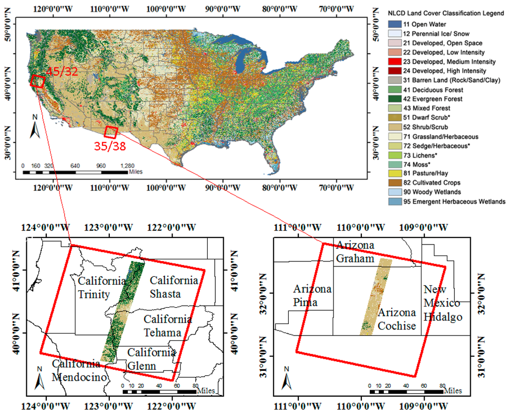
Figure 1. Landsat data areas used in this study based on the NLCD 2011 in the conterminous United States.

Table 1. Data acquired in Day of Year (DOY) format for two regions during four seasons.

Seasons	Path/Row: 45/32		Path/Row: 35/38
	Landsat 7 ETM+	Landsat 8 OLI	Landsat 7 ETM+	Landsat 8 OLI
Spring	LE72013121 (1 May 2013)	LC8 2013113 (24 April 2013)	LE7 2014070 (11 March 2014)	LC8 2014078 (19 March 2014)
Summer	LE7 2013201 (20 July 2013)	LC8 2013193 (12 July 2013)	LE7 2014182 (1 July 2014)	LC8 2014174 (23 June 2014)
Autumn	LE7 2013249 (6 September 2013)	LC8 2013257 (12 September 2013)	LE7 2013275 (2 October 2013)	LC8 2013267 (24 September 2013)
Winter	LE7 2013329 (25 November 2013)	LC8 2013337 (3 December 2013)	LE7 2014006 (6 January 2014)	LC8 2014014 (14 January 2014)

Table 1. Data acquired in Day of Year (DOY) format for two regions during four seasons.

Seasons	Path/Row: 45/32		Path/Row: 35/38
	Landsat 7 ETM+	Landsat 8 OLI	Landsat 7 ETM+	Landsat 8 OLI
Spring	LE72013121 (1 May 2013)	LC8 2013113 (24 April 2013)	LE7 2014070 (11 March 2014)	LC8 2014078 (19 March 2014)
Summer	LE7 2013201 (20 July 2013)	LC8 2013193 (12 July 2013)	LE7 2014182 (1 July 2014)	LC8 2014174 (23 June 2014)
Autumn	LE7 2013249 (6 September 2013)	LC8 2013257 (12 September 2013)	LE7 2013275 (2 October 2013)	LC8 2013267 (24 September 2013)
Winter	LE7 2013329 (25 November 2013)	LC8 2013337 (3 December 2013)	LE7 2014006 (6 January 2014)	LC8 2014014 (14 January 2014)

All Landsat images used in this study were provided by the U.S. Geological Survey (USGS) (http://earthexplorer.usgs.gov/) and downloaded as Surface Reflectance (SR) products. SR products are applications-ready data sets that have been post-production processed and include geometric rectification, atmospheric correction and other modifications (see the Landsat surface reflectance products: http://landsat.usgs.gov/CDR_LSR.php). The Landsat images include not only all the spectral bands but also the Quality Assessment (QA) band of cloud, water, shadow, snow, or filled values. The data acquired for ETM+ and OLI were 8 days apart due to the orbit of Landsat 8.

To analyze the continuity of VIs based on Landsat on-orbit data, four sets of Landsat data (both ETM+ and OLI) for two regions among the two area time series datasets were chosen to represent the four seasons (see Table 1).

3. Methodology

A comparison of the continuity of VIs derived from Landsat 8 OLI and Landsat 7 ETM+ data among vegetation types was undertaken using ground spectral data and satellite data (Figure 2). For the satellite data in the figure, pink represents OLI data while red represents ETM+ data. The letters a–f represents the six land cover types. The cells in the lower right corner, describing R² values, range from blue to red (small to large). The cells form into four pictures representing the four seasons, respectively. For each picture, the vertical axis indicates the six land cover classes while the horizontal axis indicates the five VIs.

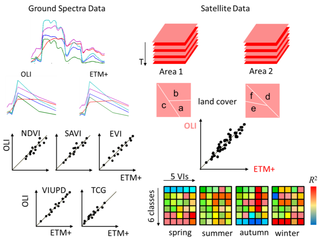
Figure 2. Our method of evaluating the continuity of VIs derived from simulated data (left) and satellite data (right).

Figure 2. Our method of evaluating the continuity of VIs derived from simulated data (left) and satellite data (right).

3.1. Simulated Data Process

The purpose of ground measured hyperspectral data is to assess the effect of sensor band pass settings with spectral convolution on the target sensors [40]. For the purpose of simulation, it was assumed that the atmosphere has no effect on radiance transfer, i.e., it is a vacuum environment. Spectral convolution is the process of spectra resampling (see [18]). Because the spectral response of each sensor has minor differences (Figure 3), the SRF measured by the sensors' calibration laboratory describes resampling as in the following equation.

$$R_{simulate}(i)=\frac{{\displaystyle {\int }_{{\lambda }_s(i)}^{{\lambda }_e(i)}{S}_i(\lambda )R(\lambda )d\lambda }}{{\displaystyle {\int }_{{\lambda }_s(i)}^{{\lambda }_e(i)}{S}_i(\lambda )I(\lambda )d\lambda }}$$

(1)

where R_simulate(i) is the reflectance of band i that will be simulated, λ_s (i) and λ_e (i) are the start and end wavelength of sensor band i, respectively. S_i (λ) is the SRF of sensor band i with wavelength λ, R(λ) is the measured reflected radiation at the top of the canopy as a function of wavelength of λ, and I(λ)is the corresponding incident radiance measured on an ideal reference panel.

The SRFs for ETM+ and OLI sensors were downloaded through the USGS (http://landsat.usgs.gov/instructions.php) and are shown in Figure 3. In general, the bandwidths of OLI are narrower than the corresponding bandwidths of ETM+. Our study focused on vegetation. A major difference was apparent in the OLI near-infrared band (NIR: 0.845–0.885 μm), which excluded a water vapor absorption feature at 0.825 μm that was obtained in the ETM+ NIR band (0.775–0.900 μm). As a reference to clarify the wavelength of the Landsat sensors corresponding to the vegetation spectra, a vegetation spectra (a deciduous forest spectra with a 2 nm spectral sampling interval) was selected from the ENVI spectral library (the Johns Hopkins University (JHU) vegetation spectral library). As soon as the at-sensor simulated reflectance was achieved through the spectral convolution of 393 ground spectral samples, the five VIs were calculated to quantitatively evaluate the continuity between OLI and ETM+ (Figure 2).

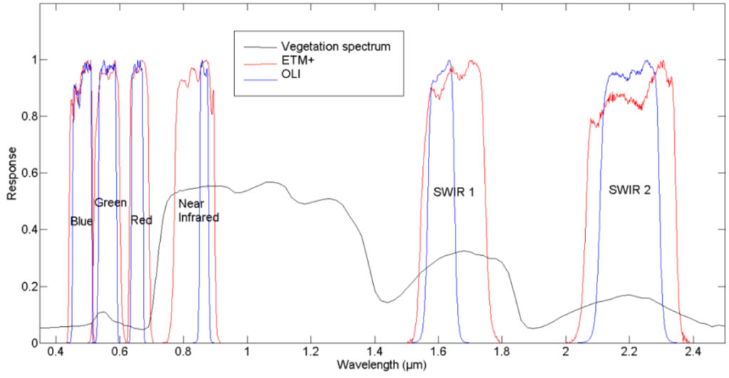
Figure 3. Spectral response function (SRF) associated with the visible, near-infrared (NIR) and shortwave infrared (SWIR) bands of the ETM+ and OLI. Red lines indicate the ETM+ sensor and blue lines indicate the OLI sensor. The black line indicates a deciduous forest spectrum as a reference.

Figure 3. Spectral response function (SRF) associated with the visible, near-infrared (NIR) and shortwave infrared (SWIR) bands of the ETM+ and OLI. Red lines indicate the ETM+ sensor and blue lines indicate the OLI sensor. The black line indicates a deciduous forest spectrum as a reference.

3.2. Satellite Data Process

The objective of satellite data used is to evaluate the response of the different VIs among different vegetation types to the data continuity between OLI and ETM+, and also to analyze the continuity of VIs with multi-temporal data during the four seasons. Landsat satellite datasets containing the current on-orbit ETM+ and OLI data were acquired (Figure 2).

All Landsat images were downloaded as surface reflectance products via the USGS. A flow chart of the processing methods is shown in Figure 4. To improve the reliability of the results, cloud cover had to be removed from both the ETM+ and OLI images. When the cfmask band is used for quality/feature classification driven by the Landsat Cloud Cover Assessment (CCA) algorithm, clouds, snow, shadow, and the filled values can be classified, thus, the cfmask file was used during the quality control process to achieve cloud-free images. Because the ETM+ data had been degraded by the Scan Line Corrector (SLC)-off gaps since 2003, the gap-clear central parts of the images were used as a subset for this study (as shown in Figure 1). All scenes of the same sites were placed in a subset of the same size, which produced two series datasets. Combined with the NLCD 2011 classification, six vegetation cover types were extracted as regions of interest (ROIs) for each dataset, and we randomly selected 1000 samples from each ROI type by ENVI for later analysis of the relationship between OLI and ETM+ images for different land cover types during various time periods. The number of the selected samples for regression analysis was determined as 1000 based on the fact that the minimum amount of the pixel of the specified 6 land cover types is less than 2000. The statistical regression relationship (first-order linear polynomials) was calculated for all five VIs (NDVI, SAVI, EVI, VIUPD, and TCG) based on the 1000 samples of the six classes. A total of 120 records derived from five VIs of six vegetation classes and four seasons for OLI and ETM+ data (5 × 6 × 4 = 120) were analyzed in this study.

Figure 4. Flow diagram of the satellite data processing performed in this study.

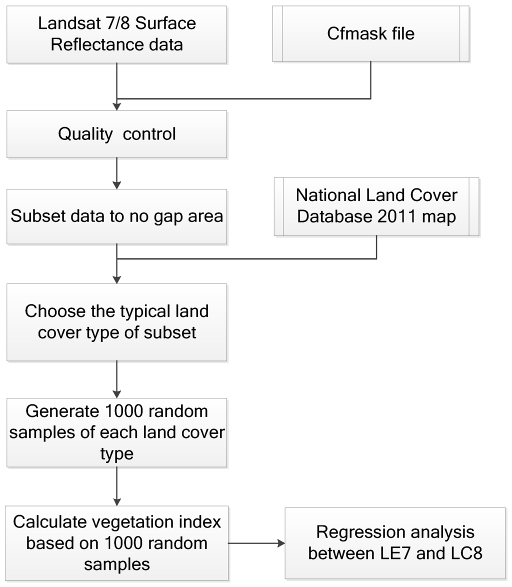
Figure 4. Flow diagram of the satellite data processing performed in this study.

3.3. Vegetation Indices

The computation rules for a VI allow two methods: band geometric computing and band transformation. In this study, we used three band-geometric-computing VIs (NDVI, SAVI, and EVI) and two band-transformation VIs (VIUPD and TCG), as shown in Table 2 [9,36,37,38,39].

VIUPD is based on the Universal Pattern Decomposition Method (UPDM) [41]. The coefficients of VIUPD can be determined using Equation (2).

$$R(i)\to C_w\cdot P_w(i)+C_v\cdot P_v(i)+C_s\cdot P_s(i)+C_4\cdot P_4(i)$$

(2)

where R(i) is the reflectance of band i for each pixel and C_W, C_V, and C_S are the decomposition coefficients (or abundance of elements). P_k(i) (k = w, v, s, 4) indicates for the universal spectra of patterns [38].

The transformation coefficients for VIUPD, P_k(i), and TCG were slightly different. VIUPD coefficients were reported for OLI in [42] and for ETM+ in [34]. TCG parameters for Landsat ETM+ and OLI followed [43,44] and are displayed in Table 2.

Table 2. Vegetation indices tested in this study.

Index	Formulation	References
NDVI	$NDVI=({\rho }_{NIR}-{\rho }_R)/({\rho }_{NIR}+{\rho }_R)$	[9]
SAVI	$SAVI=(1+L)\frac{{\rho }_{NIR}-{\rho }_{\mathrm{Re}d}}{{\rho }_{NIR}+{\rho }_{\mathrm{Re}d}+L},whereL=0.5$	[36]
EVI	$\begin{array}{l}EVI=G\times \frac{{\rho }_{NIR}-{\rho }_{\mathrm{R}}}{{\rho }_{NIR}+a\times {\rho }_{\mathrm{R}}-b\times {\rho }_B+L},\\ whereG=2.5,a=6,b=7.5,L=1\end{array}$	[37]
VIUPD	$VIUPD=\frac{C_V-a{C}_S-C_4}{C_W+C_V+C_S},wherea=0.1$	[38]
TCG	$\begin{array}{l}{\text{TCG}}_{\text{ETM\_SR}}=\text{-0.2971}\times {\rho }_{\text{blue}}\text{-0.2425}\times {\rho }_{\text{green}}\text{-0.5411}\times {\rho }_{\text{red}}\\ +\text{0.7263}\times {\rho }_{\text{NIR}}+\text{0.0718}\times {\rho }_{\text{SWIR1}}\text{-0.1658}\times {\rho }_{\text{SWIR2}}\end{array}$ $\begin{array}{l}{\text{TCG}}_{\text{OLI\_SR}}=\text{-0.2939}\times {\rho }_{\text{blue}}\text{-0.2491}\times {\rho }_{\text{green}}\text{-0.5482}\times {\rho }_{\text{red}}\\ +\text{0.7184}\times {\rho }_{\text{NIR}}+\text{0.0707 }\times {\rho }_{\text{SWIR1}}\text{-0.1729}\times {\rho }_{\text{SWIR2}}\end{array}$	[39]

Table 2. Vegetation indices tested in this study.

Index	Formulation	References
NDVI	$NDVI=({\rho }_{NIR}-{\rho }_R)/({\rho }_{NIR}+{\rho }_R)$	[9]
SAVI	$SAVI=(1+L)\frac{{\rho }_{NIR}-{\rho }_{\mathrm{Re}d}}{{\rho }_{NIR}+{\rho }_{\mathrm{Re}d}+L},whereL=0.5$	[36]
EVI	$\begin{array}{l}EVI=G\times \frac{{\rho }_{NIR}-{\rho }_{\mathrm{R}}}{{\rho }_{NIR}+a\times {\rho }_{\mathrm{R}}-b\times {\rho }_B+L},\\ whereG=2.5,a=6,b=7.5,L=1\end{array}$	[37]
VIUPD	$VIUPD=\frac{C_V-a{C}_S-C_4}{C_W+C_V+C_S},wherea=0.1$	[38]
TCG	$\begin{array}{l}{\text{TCG}}_{\text{ETM\_SR}}=\text{-0.2971}\times {\rho }_{\text{blue}}\text{-0.2425}\times {\rho }_{\text{green}}\text{-0.5411}\times {\rho }_{\text{red}}\\ +\text{0.7263}\times {\rho }_{\text{NIR}}+\text{0.0718}\times {\rho }_{\text{SWIR1}}\text{-0.1658}\times {\rho }_{\text{SWIR2}}\end{array}$ $\begin{array}{l}{\text{TCG}}_{\text{OLI\_SR}}=\text{-0.2939}\times {\rho }_{\text{blue}}\text{-0.2491}\times {\rho }_{\text{green}}\text{-0.5482}\times {\rho }_{\text{red}}\\ +\text{0.7184}\times {\rho }_{\text{NIR}}+\text{0.0707 }\times {\rho }_{\text{SWIR1}}\text{-0.1729}\times {\rho }_{\text{SWIR2}}\end{array}$	[39]

4. Results

4.1. Continuity of VIs Derived from Simulated Data

A total of 393 ground measured spectral samples were simulated to the Landsat ETM+ and OLI at-sensor reflectance value according to the SRF of the target sensor. VIs derived from the simulated broad bands were analyzed by linear regression between OLI and ETM+ (Figure 5).

VIs derived from OLI and ETM+ had a strong linear relationship, as is evident in Figure 5. Based on the simulated data, the coefficients of determination (R²) between OLI and ETM+ ranged from 0.99767 (TCG) to 0.99971 (VIUPD). As a result, the continuity of VIs in OLI and its predecessor was shown to be high in the simulated situation. The ground data simulation experiment accounted for only the impact of the band-pass settings of the sensors, which reflects the fact that OLI largely inherited the design of its predecessor Landsat sensor in the field of VI calculation. This provided a theoretical basis for the following satellite data analysis.

4.2. Continuity of VIs Derived from Satellite Data

As mentioned in the Data section, 40 scenes for Landsat WRS-2 45/32 (path/row) and 44 scenes for 35/38 (path/row) were chosen. Using NDVI as an example, the time series profiles for six vegetation cover types (evergreen forest, deciduous forest and mixed forest in the 45/32 area; shrub, grassland and cultivated crops in the 35/38 area) are displayed in Figure 6. OLI data are linked by solid lines and ETM+ data are linked by dash lines. Since data collection by ETM+ and OLI was 8 days apart, we selected a relatively steady period from each season to minimize the impact of the 8-day offset on the results. The dates of the four pairs images from both Landsat 8 OLI and Landsat 7 ETM+ data are given in Table 1.

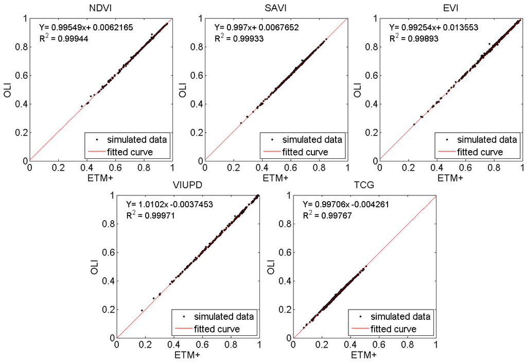
Figure 5. Correlations among vegetation indices (NDVI, SAVI, EVI, VIUPD, and TCG,) determined using ETM+-derived data (x-axis)- and OLI-derived data (y-axis). Data was spectrally convoluted from ground measured spectra (number of samples = 393) to at-sensor reflectance.

Figure 5. Correlations among vegetation indices (NDVI, SAVI, EVI, VIUPD, and TCG,) determined using ETM+-derived data (x-axis)- and OLI-derived data (y-axis). Data was spectrally convoluted from ground measured spectra (number of samples = 393) to at-sensor reflectance.

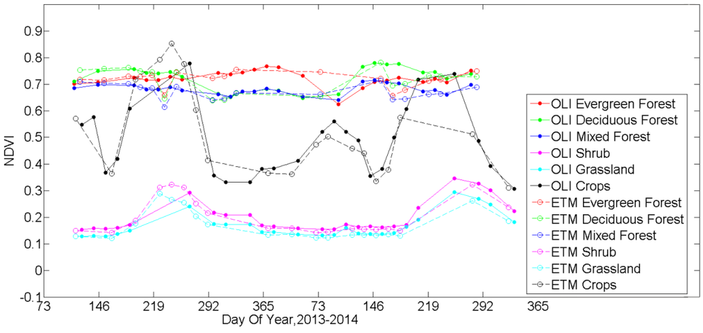
Figure 6. NDVI time series profiles calculated by Landsat OLI (solid lines with circles) and ETM+ (dash lines with hollow circles) data for the six vegetation classes used in this study in different colors. Each profile was averaged from 1000 samples extracted from each class.

Figure 6. NDVI time series profiles calculated by Landsat OLI (solid lines with circles) and ETM+ (dash lines with hollow circles) data for the six vegetation classes used in this study in different colors. Each profile was averaged from 1000 samples extracted from each class.

The scatterplots of the five VIs derived from ETM+ (x-axis) and OLI (y-axis) for three forest areas and three non-forest areas are shown in Figure 7 and Figure 8, respectively. Six vegetation cover types in four seasons for five VIs resulted in 120 records in total. Because each record contained 1000 random samples, which are too crowd to plot, data displayed on the scatterplots were selected in five step lengths (one sample from every five samples). The step length was determined after several tests trying not only to maintain the samples’ integrity but to ensure the aesthetics of the scatterplots at the same time. As a result, the data size was reduced from 1000 to 200 for each record. The reduced 200 samples was only used for viewing, with all 1000 random samples used for the statistical analysis.

Figure 7. Scatterplots showing the correlational relationships among five VIs as derived from Landsat 7 ETM+ and Landsat 8 OLI data for three forest types during the four seasons. Among the 12 scatterplots, deciduous forest, evergreen forest, and mixed forest are shown on the vertical axis, with spring, summer, autumn, and winter on the horizontal axis.

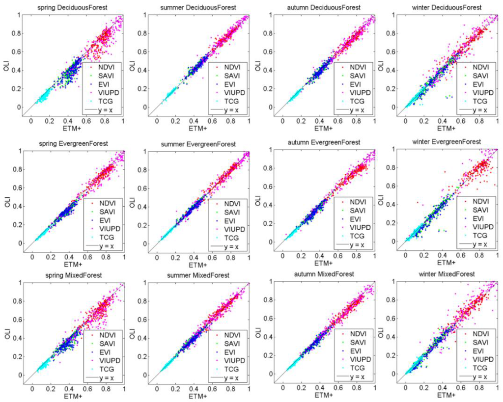
Figure 7. Scatterplots showing the correlational relationships among five VIs as derived from Landsat 7 ETM+ and Landsat 8 OLI data for three forest types during the four seasons. Among the 12 scatterplots, deciduous forest, evergreen forest, and mixed forest are shown on the vertical axis, with spring, summer, autumn, and winter on the horizontal axis.

The VIs of the three forest types were markedly higher than for the non-forest land cover types, with the exception of crops. For clarity, the X- and Y-axis maxima for forests were set to 1, while those of the non-forests were set to 0.5. The linear relationship equations for each VI derived from every 1000 random samples for each vegetation class in each season are displayed in Table 3. The determination coefficients (R²) based on the linear correlations of the five VIs derived from ETM+ and OLI data for the four seasons are shown in Table 4. The red color indicates the highest correlation, and green indicates the lowest correlation. For each record, 1000 random samples were used in the regression evaluation.

Figure 8. Scatterplots showing the correlational relationships among five VIs as derived from Landsat 7 ETM+ and Landsat 8 OLI data for three non-forest types during the four seasons. Among the 12 scatterplots, shrub, grassland, crops are shown on the vertical axis, with spring, summer, autumn, and winter on the horizontal axis.

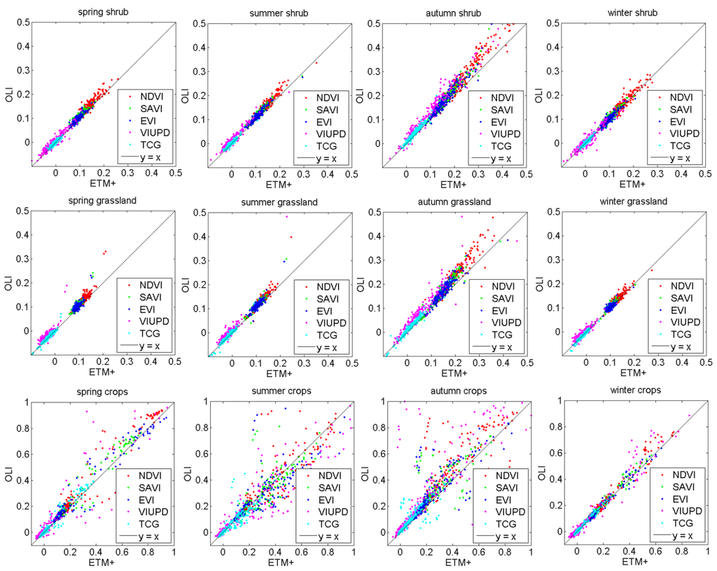
Figure 8. Scatterplots showing the correlational relationships among five VIs as derived from Landsat 7 ETM+ and Landsat 8 OLI data for three non-forest types during the four seasons. Among the 12 scatterplots, shrub, grassland, crops are shown on the vertical axis, with spring, summer, autumn, and winter on the horizontal axis.

4.2.1. Analysis of the Generation Algorithm for VIs

Among the four seasons and six land cover classes (24 records), VIUPD had the highest coefficient of determination (R²) (13/24). TCG was also very consistent between ETM+ and OLI (9/24). Overall, band-transformation-derived VIs (VIUPD and TCG) displayed greater consistency between the ETM+ and OLI sensors (higher R²), and had a greater consistency than the geometric-computation VIs (NDVI, SAVI, and EVI).

VI distributions differed markedly among the different vegetation classes. This is qualitatively demonstrated in Figure 7 and Figure 8. Moreover, Figure 9 shows the distributions of the five VIs in each vegetation class by using quantitative boxplots. The boxplot contains multi-variations, including the first quartile (bottom of the box), the second quartile (the median), the third quartile (top of the box), and the ends of the whiskers (minima and maxima). Each vegetation type had unique growth characteristics that affected the VI response. In the three forest types, VIUPD and NDVI medians distributions were similar, ranging from 0.6 to 0.8, and were considerably higher than for the other VIs (Figure 9a–c). For both the forest and non-forest land cover types, SAVI and EVI had a similar performance, as seen in Figure 9. TCG had the lowest values among the five VIs (Figure 9).

Table 3. Linear regression equations (Y = a x + b) of the VIs derived from ETM+ and OLI data for six vegetation classes in four seasons. Y is the OLI data and x is the ETM+ data.

--		NDVI	SAVI	EVI	VIUPD	TCG
Spring	Deciduous Forest	Y = 0.97 x − 0.017	Y = 0.98 x − 0.027	Y = 0.95 x − 0.024	Y = 1.03 x − 0.095	Y = 0.91 x − 0.015
	Evergreen Forest	Y = 0.93 x + 0.029	Y = 0.94 x + 0.003	Y = 0.92 x + 0.005	Y = 0.96 x + 0.004	Y = 0.88 x − 0.003
	Mixed Forest	Y = 0.89 x + 0.052	Y = 0.91 x + 0.010	Y = 0.89 x + 0.009	Y = 0.94 x − 0.003	Y = 0.85 x − 0.0003
	Shrub	Y = 0.96 x + 0.015	Y = 0.95 x + 0.014	Y = 0.94 x + 0.012	Y = 0.92 x + 0.007	Y = 0.98 x − 0.008
	Grassland	Y = 1.12 x − 0.001	Y = 1.10 x + 0.001	Y = 1.05 x + 0.004	Y = 1.10 x + 0.014	Y = 1.17 x − 0.013
	Crops	Y = 1.06 x + 0.017	Y = 1.10 x + 0.014	Y = 0.98 x + 0.021	Y = 1.07 x + 0.025	Y = 1.03 x − 0.004
Summer	Deciduous Forest	Y = 0.95 x + 0.047	Y = 0.996 x + 0.01	Y = 0.98 x + 0.011	Y = 0.99 x + 0.018	Y = 0.96 x + 0.001
	Evergreen Forest	Y = 0.98 x + 0.011	Y = 1.01 x − 0.002	Y = 0.99 x − 0.003	Y = 0.995 x − 0.008	Y = 0.97 x − 0.004
	Mixed Forest	Y = 0.92 x + 0.060	Y = 0.97 x + 0.018	Y = 0.97 x + 0.011	Y = 0.97 x + 0.020	Y = 0.93 x + 0.003
	Shrub	Y = 1.06 x + 0.006	Y = 1.05 x + 0.005	Y = 1.03 x + 0.005	Y = 1.03 x + 0.013	Y = 1.02 x − 0.008
	Grassland	Y = 0.87 x + 0.030	Y = 0.82 x + 0.030	Y = 0.73 x + 0.04	Y = 0.79 x + 0.010	Y = 0.99 x − 0.013
	Crops	Y = 0.85 x + 0.053	Y = 0.81 x + 0.051	Y = 0.72 x + 0.06	Y = 0.75 x + 0.044	Y = 0.79 x + 0.005
Autumn	Deciduous Forest	Y = 0.93 x + 0.035	Y = 1.00 x − 0.012	Y = 0.997 x − 0.01	Y = 0.95 x + 0.020	Y = 0.94 x − 0.008
	Evergreen Forest	Y = 0.89 x + 0.056	Y = 1.02 x − 0.022	Y = 1.01 x − 0.021	Y = 0.93 x + 0.032	Y = 0.96 x − 0.011
	Mixed Forest	Y = 0.90 x + 0.055	Y = 0.97 x + 0.001	Y = 0.98 x − 0.005	Y = 0.94 x + 0.027	Y = 0.91 x − 0.002
	Shrub	Y = 1.18 x − 0.004	Y = 1.19 x − 0.006	Y = 1.16 x − 0.005	Y = 1.17 x + 0.017	Y = 1.17 x − 0.008
	Grassland	Y = 1.17 x + 0.003	Y = 1.10 x + 0.010	Y = 1.02 x + 0.019	Y = 1.09 x + 0.028	Y = 1.20 x − 0.011
	Crops	Y = 0.87 x + 0.125	Y = 0.81 x + 0.094	Y = 0.75 x + 0.105	Y = 0.84 x + 0.124	Y = 0.78 x + 0.030
Winter	Deciduous Forest	Y = 0.90 x + 0.072	Y = 1.07 x − 0.023	Y = 1.03 x − 0.021	Y = 0.98 x + 0.037	Y = 0.995 x − 0.006
	Evergreen Forest	Y = 0.79 x + 0.157	Y = 1.09 x − 0.034	Y = 1.06 x − 0.032	Y = 0.92 x + 0.102	Y = 1.01 x − 0.010
	Mixed Forest	Y = 0.88 x + 0.086	Y = 1.08 x − 0.024	Y = 1.05 x − 0.024	Y = 0.98 x + 0.036	Y = 1.00 x − 0.006
	Shrub	Y = 1.00 x + 0.008	Y = 0.99 x + 0.006	Y = 0.94 x + 0.008	Y = 0.92 x + 0.004	Y = 1.01 x − 0.009
	Grassland	Y = 0.97 x + 0.012	Y = 0.95 x + 0.011	Y = 0.89 x + 0.014	Y = 0.96 x + 0.007	Y = 1.08 x − 0.014
	Crops	Y = 1.06 x + 0.002	Y = 1.04 x + 0.005	Y = 0.98 x + 0.009	Y = 1.07 x + 0.008	Y = 1.03 x − 0.009

Table 3. Linear regression equations (Y = a x + b) of the VIs derived from ETM+ and OLI data for six vegetation classes in four seasons. Y is the OLI data and x is the ETM+ data.

--		NDVI	SAVI	EVI	VIUPD	TCG
Spring	Deciduous Forest	Y = 0.97 x − 0.017	Y = 0.98 x − 0.027	Y = 0.95 x − 0.024	Y = 1.03 x − 0.095	Y = 0.91 x − 0.015
	Evergreen Forest	Y = 0.93 x + 0.029	Y = 0.94 x + 0.003	Y = 0.92 x + 0.005	Y = 0.96 x + 0.004	Y = 0.88 x − 0.003
	Mixed Forest	Y = 0.89 x + 0.052	Y = 0.91 x + 0.010	Y = 0.89 x + 0.009	Y = 0.94 x − 0.003	Y = 0.85 x − 0.0003
	Shrub	Y = 0.96 x + 0.015	Y = 0.95 x + 0.014	Y = 0.94 x + 0.012	Y = 0.92 x + 0.007	Y = 0.98 x − 0.008
	Grassland	Y = 1.12 x − 0.001	Y = 1.10 x + 0.001	Y = 1.05 x + 0.004	Y = 1.10 x + 0.014	Y = 1.17 x − 0.013
	Crops	Y = 1.06 x + 0.017	Y = 1.10 x + 0.014	Y = 0.98 x + 0.021	Y = 1.07 x + 0.025	Y = 1.03 x − 0.004
Summer	Deciduous Forest	Y = 0.95 x + 0.047	Y = 0.996 x + 0.01	Y = 0.98 x + 0.011	Y = 0.99 x + 0.018	Y = 0.96 x + 0.001
	Evergreen Forest	Y = 0.98 x + 0.011	Y = 1.01 x − 0.002	Y = 0.99 x − 0.003	Y = 0.995 x − 0.008	Y = 0.97 x − 0.004
	Mixed Forest	Y = 0.92 x + 0.060	Y = 0.97 x + 0.018	Y = 0.97 x + 0.011	Y = 0.97 x + 0.020	Y = 0.93 x + 0.003
	Shrub	Y = 1.06 x + 0.006	Y = 1.05 x + 0.005	Y = 1.03 x + 0.005	Y = 1.03 x + 0.013	Y = 1.02 x − 0.008
	Grassland	Y = 0.87 x + 0.030	Y = 0.82 x + 0.030	Y = 0.73 x + 0.04	Y = 0.79 x + 0.010	Y = 0.99 x − 0.013
	Crops	Y = 0.85 x + 0.053	Y = 0.81 x + 0.051	Y = 0.72 x + 0.06	Y = 0.75 x + 0.044	Y = 0.79 x + 0.005
Autumn	Deciduous Forest	Y = 0.93 x + 0.035	Y = 1.00 x − 0.012	Y = 0.997 x − 0.01	Y = 0.95 x + 0.020	Y = 0.94 x − 0.008
	Evergreen Forest	Y = 0.89 x + 0.056	Y = 1.02 x − 0.022	Y = 1.01 x − 0.021	Y = 0.93 x + 0.032	Y = 0.96 x − 0.011
	Mixed Forest	Y = 0.90 x + 0.055	Y = 0.97 x + 0.001	Y = 0.98 x − 0.005	Y = 0.94 x + 0.027	Y = 0.91 x − 0.002
	Shrub	Y = 1.18 x − 0.004	Y = 1.19 x − 0.006	Y = 1.16 x − 0.005	Y = 1.17 x + 0.017	Y = 1.17 x − 0.008
	Grassland	Y = 1.17 x + 0.003	Y = 1.10 x + 0.010	Y = 1.02 x + 0.019	Y = 1.09 x + 0.028	Y = 1.20 x − 0.011
	Crops	Y = 0.87 x + 0.125	Y = 0.81 x + 0.094	Y = 0.75 x + 0.105	Y = 0.84 x + 0.124	Y = 0.78 x + 0.030
Winter	Deciduous Forest	Y = 0.90 x + 0.072	Y = 1.07 x − 0.023	Y = 1.03 x − 0.021	Y = 0.98 x + 0.037	Y = 0.995 x − 0.006
	Evergreen Forest	Y = 0.79 x + 0.157	Y = 1.09 x − 0.034	Y = 1.06 x − 0.032	Y = 0.92 x + 0.102	Y = 1.01 x − 0.010
	Mixed Forest	Y = 0.88 x + 0.086	Y = 1.08 x − 0.024	Y = 1.05 x − 0.024	Y = 0.98 x + 0.036	Y = 1.00 x − 0.006
	Shrub	Y = 1.00 x + 0.008	Y = 0.99 x + 0.006	Y = 0.94 x + 0.008	Y = 0.92 x + 0.004	Y = 1.01 x − 0.009
	Grassland	Y = 0.97 x + 0.012	Y = 0.95 x + 0.011	Y = 0.89 x + 0.014	Y = 0.96 x + 0.007	Y = 1.08 x − 0.014
	Crops	Y = 1.06 x + 0.002	Y = 1.04 x + 0.005	Y = 0.98 x + 0.009	Y = 1.07 x + 0.008	Y = 1.03 x − 0.009

Table 4. Coefficient of determination (R²) of the regression relationships for the VIs as derived from ETM+ and OLI data for six vegetation classes for the four seasons. A three-color gradient (green-yellow-red) is used to colorize the R² value in each cell from small to large.

Seasons	Vegetation Types	NDVI	SAVI	EVI	VIUPD	TCG
Spring	Deciduous Forest	0.7421	0.7364	0.734	0.7968	0.7609
	Evergreen Forest	0.9314	0.9117	0.9015	0.9502	0.9201
	Mixed Forest	0.8031	0.8234	0.8263	0.8616	0.8376
	Shrub	0.8898	0.8299	0.8312	0.9199	0.883
	Grassland	0.9411	0.9406	0.9362	0.9486	0.9616
	crops	0.9442	0.9487	0.9503	0.9518	0.9512
Summer	Deciduous Forest	0.9272	0.9326	0.9187	0.9584	0.936
	Evergreen Forest	0.9606	0.9623	0.9527	0.9736	0.9643
	Mixed Forest	0.9294	0.9498	0.9444	0.9621	0.9561
	Shrub	0.9155	0.9008	0.9004	0.9339	0.9176
	Grassland	0.8659	0.8694	0.8596	0.8692	0.9333
	crops	0.7475	0.6799	0.6277	0.6675	0.657
Autumn	Deciduous Forest	0.9252	0.937	0.9247	0.9564	0.9441
	Evergreen Forest	0.9403	0.9402	0.9347	0.9642	0.9492
	Mixed Forest	0.9453	0.9561	0.9501	0.9685	0.96
	Shrub	0.9503	0.9425	0.9376	0.9615	0.9468
	Grassland	0.8847	0.839	0.7692	0.8201	0.9217
	crops	0.6376	0.6038	0.5847	0.5768	0.6103
Winter	Deciduous Forest	0.8317	0.9311	0.9266	0.9072	0.9407
	Evergreen Forest	0.6968	0.9446	0.9407	0.8408	0.9552
	Mixed Forest	0.8016	0.9622	0.9564	0.886	0.9652
	Shrub	0.8768	0.841	0.8184	0.8818	0.899
	Grassland	0.9215	0.9171	0.9164	0.9535	0.9589
	crops	0.9716	0.9773	0.9771	0.957	0.9773

Table 4. Coefficient of determination (R²) of the regression relationships for the VIs as derived from ETM+ and OLI data for six vegetation classes for the four seasons. A three-color gradient (green-yellow-red) is used to colorize the R² value in each cell from small to large.

Seasons	Vegetation Types	NDVI	SAVI	EVI	VIUPD	TCG
Spring	Deciduous Forest	0.7421	0.7364	0.734	0.7968	0.7609
	Evergreen Forest	0.9314	0.9117	0.9015	0.9502	0.9201
	Mixed Forest	0.8031	0.8234	0.8263	0.8616	0.8376
	Shrub	0.8898	0.8299	0.8312	0.9199	0.883
	Grassland	0.9411	0.9406	0.9362	0.9486	0.9616
	crops	0.9442	0.9487	0.9503	0.9518	0.9512
Summer	Deciduous Forest	0.9272	0.9326	0.9187	0.9584	0.936
	Evergreen Forest	0.9606	0.9623	0.9527	0.9736	0.9643
	Mixed Forest	0.9294	0.9498	0.9444	0.9621	0.9561
	Shrub	0.9155	0.9008	0.9004	0.9339	0.9176
	Grassland	0.8659	0.8694	0.8596	0.8692	0.9333
	crops	0.7475	0.6799	0.6277	0.6675	0.657
Autumn	Deciduous Forest	0.9252	0.937	0.9247	0.9564	0.9441
	Evergreen Forest	0.9403	0.9402	0.9347	0.9642	0.9492
	Mixed Forest	0.9453	0.9561	0.9501	0.9685	0.96
	Shrub	0.9503	0.9425	0.9376	0.9615	0.9468
	Grassland	0.8847	0.839	0.7692	0.8201	0.9217
	crops	0.6376	0.6038	0.5847	0.5768	0.6103
Winter	Deciduous Forest	0.8317	0.9311	0.9266	0.9072	0.9407
	Evergreen Forest	0.6968	0.9446	0.9407	0.8408	0.9552
	Mixed Forest	0.8016	0.9622	0.9564	0.886	0.9652
	Shrub	0.8768	0.841	0.8184	0.8818	0.899
	Grassland	0.9215	0.9171	0.9164	0.9535	0.9589
	crops	0.9716	0.9773	0.9771	0.957	0.9773

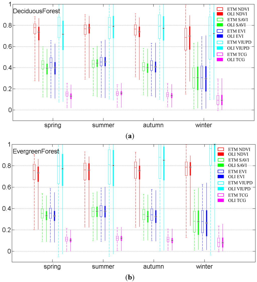
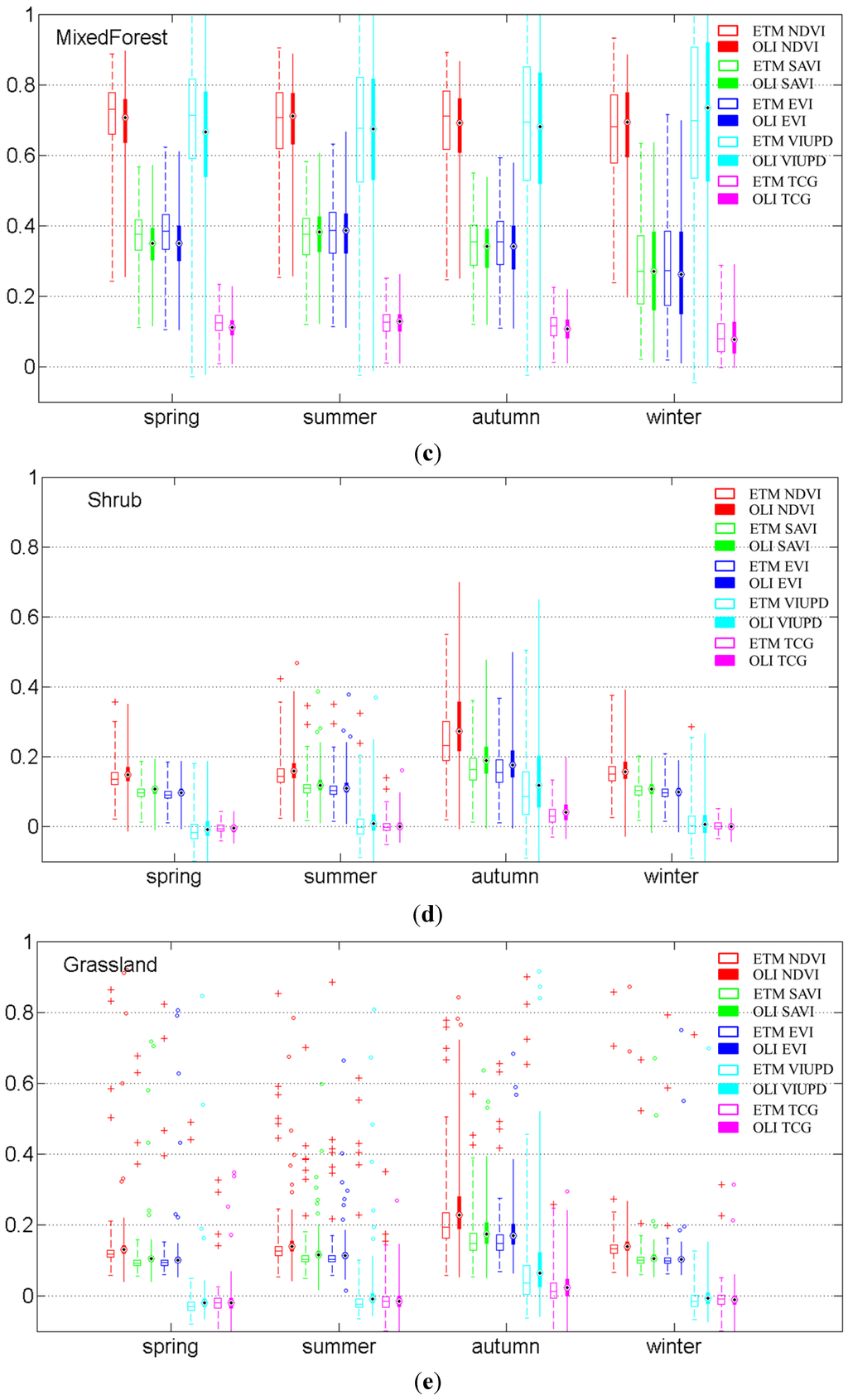
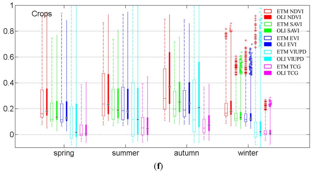
Figure 9. The VIs of various vegetation types during the four seasons based on ETM+ and OLI data. The hollow boxes indicate ETM+ -derived VIs and the solid boxes indicate OLI-derived VIs. The five VIs are shown in red, green, blue, cyan and magenta. (a) Deciduous forest; (b) Evergreen forest; (c) Mixed forest; (d) Shrub; (e) Grassland; (f) Crops.

Figure 9. The VIs of various vegetation types during the four seasons based on ETM+ and OLI data. The hollow boxes indicate ETM+ -derived VIs and the solid boxes indicate OLI-derived VIs. The five VIs are shown in red, green, blue, cyan and magenta. (a) Deciduous forest; (b) Evergreen forest; (c) Mixed forest; (d) Shrub; (e) Grassland; (f) Crops.

4.2.2. The Response of VIs to Growth Variation

For each vegetation cover type, the results of the VIs varied between the different seasons. For the three forest types, VI continuity between the two sensors was higher in summer and autumn (average R² > 0.93) than in winter or spring. Forests in the Northern Hemisphere experience moderate growth in summer and autumn. Figure 6 shows that deciduous forest exhibited a slight seasonal response (growth started from 12 April 2013 and ended at 1 November 2013). The time series profiles show that evergreen and mixed forests were less variable compared with deciduous forest. However, the date of initiation or cessation of the growth period varied according to the tree variety, especially for deciduous forests. This can be seen in Figure 9a–c, which shows the VI distribution at various times. For deciduous forest in spring (24 April and 1 May 2013), the average VI values displayed a relatively large difference between OLI and ETM+ (Figure 9a) values. The R² values were relatively low (mean R² = 0.7540). During winter (25 November and 3 December 2013), when the photosynthetic capacity of trees gradually begins to weaken, VI variation was more significant than during the other seasons in all three forest types (Figure 9a–c). The consistency of VIs was lower in winter (mean R² = 0.9075 for deciduous forest, mean R² = 0.8756 for evergreen forest, mean R² = 0.9143 for mixed forest). In summary, VI consistency was lower during periods of relatively slow growth (winter and spring) than in periods of relatively rapid growth (summer and autumn) for all tree species.

For shrubs, R² was 0.8708 in spring, 0.9136 in summer, 0.9477 in autumn, and 0.8634 in winter. The trends in consistency were similar to those of forests, although the vegetation density was much lower than in forests, as shown in Figure 6 and Figure 9d. In addition to the factors that influenced the forests, the soil background also influenced the results for shrub. For the shrubs, this factor had a less-marked influence on VI continuity when growth was most rapid.

In contrast to the forests and shrub land cover types, VI continuity in summer and autumn was lower than in winter and spring for grassland (mean R² = 0.9456 in spring, mean R² = 0.9335 in winter) and crops (mean R² = 0.9492 in spring, mean R² = 0.9721 in winter). For grassland, VI values were very low (mostly below 0.2) as shown in Figure 9e. Therefore, the vegetation cover ratio was extremely low and the soil background strongly affected the VIs. Consequently, the VI correlation relationship was high when green grass became dry grass, which has spectral characteristics similar to those of soil. Cultivated-crop-area-derived VIs varied with the phenology (Figure 6), except in winter following the harvesting of crops or replanting with new crops. The most remarkable fluctuations were found for cultivated crops (final row in Figure 8). In Figure 9f, there are many outliers for crop VIs during the winter period, which indicates that the growth state of some crops changed considerably. Figure 6 shows that crops experienced two growth peaks during a single year: a small peak in spring and a large peak in autumn. Since the 35/38 area was located in the Great Plains region of the U.S., it contained crops of several classes [45], which have different phenologies.

5. Discussion

Landsat 8, a recently launched satellite, aims to provide the data continuity for the Landsat and has attracted the interests of land surface time series researchers. The purpose of this study was to evaluate the continuity of band-geometric and band-transformation derived VIs from Landsat 7 ETM+ and Landsat 8 OLI across seasons and different vegetation cover types with respect to differences in band-pass, VI algorithms, and sensor characteristics.

The results from ground measured data showed that the difference in VIs due to the band-pass differences between OLI and ETM+ can be neglected under ideal circumstance. Furthermore, the satellite data showed that the continuity of VIs derived by band-transformation (VIUPD and TCG) was greater than that of VIs derived by band-geometric algorithms (NDVI, SAVI, and EVI). There have been few previous studies that have compared the continuity of multi-sensors with a consideration of VI algorithms. And therefore, this study could become a useful reference. VIUPD produced the best R² values, indicating that it was less sensor dependent. Previous studies of VIUPD consistency between Hyperion and the Compact High Resolution Imaging Spectrometer (CHRIS), and between the Moderate Resolution Imaging Spectrometer (MODIS) and thematic mapper (TM) have been reported [21,34]. Both studies reported that VIUPD had a high consistency among the different platform sensors, which is consistent with our results. VIUPD has been applied more commonly for hyperspectral data than multispectral data, and this study has extended its use to series multispectral datasets, such as Landsat. Furthermore, VIUPD also functions well using different sensors in the same mission series--Landsat, as indicated by the subtle differences detected.

The five VIs responded differently towards the vegetation cover types. VIUPD and NDVI values were considerably higher than the other VIs in the area with high vegetation density such as forests (Figure 9a–c). Due to the scaling problem, NDVI is easily saturated in areas with high vegetation cover [7]. It was assumed that VIUPD was equal to 1 when the target was covered by green vegetation which explains the high values [38]. The distributions of VIUPD values among the three non-forest types were different from the three forest types. It turned out that VIUPD can also characterize the growing status information of target in conditions with low vegetation cover (Figure 9d–f). This is because VIUPD contains the standard soil pattern, which enables the effect of the soil background to be eliminated. The wide range of VIUPD allows this metric to provide more information on the states of vegetation. All of the bands used to derive VIUPD were selected to reduce atmospheric effects and be more sensitive to water content. In conclusion, VIUPD is sensitive to both high and low-density vegetation cover. The EVI and SAVI values were similar and were intermediate among the five VIs. EVI is modified on the basis of SAVI to eliminate atmospheric effects by combining the blue and red bands instead of using only the red band and it shares the same value domains as SAVI. TCG produced the lowest value. Among the ETM+ and OLI surface reflectance parameters for TCG, there were a number of negative values, which led to the relatively low result for the value domain.

It should be noted that there are other possible sources of variation between the paired images of OLI and ETM+ used here including over-pass time, scanning system, angular affect, and etc. [20]. On one hand, the ratio concept used in VIs makes it possible to reduce many forms of multiplicative noise (illumination differences, atmospheric attenuation, topographic variations to a certain degree). On the other hand, the acquisition times of OLI and ETM+ images in pairs are a few minutes apart, and the solar angles are nearly the same according to the metadata. We used the central part of each scene to reduce the ETM+ SLC-off impacts and also the angular affects. Roy et al. (2008) stated that the Landsat sensors are not as severely affected by the effects of viewing angle variations as MODIS because of its comparatively narrow field of view [46].

In this study, the effect of 8-day gap between OLI and ETM+ data on the comparison was assumed to be negligible. In general, the values acquired by sensors can vary during 8 days interval because the land cover type changed or the growth status of covered vegetation changed. As shown in Figure 6, the growth of forests, shrubs and grasslands were extremely slow that we assumed the effects of the 8 days on the results to be negligible. Although the growth of cultivated crops changed more rapidly than other vegetation types, as can be seen from the divergent scatterplots in Figure 8 or the corresponding R² in Table 4, the 8-day timing factor together with other factors mentioned above influencing the results for crops. Thus it is hardly to assess the 8-day timing influence separately, let alone the phonological variation. To reduce the 8 days influences possible, this study selected the steady growth periods in four seasons (Table 1) for the six land cover types.

The difference between the data from NLCD 2011 as classification reference and the satellite data from 2013 and 2014 are negligible in this study. It is for sure that land cover might have changed from 2011 to 2014 more or less. But unlike the urban changes annually, our study focused on areas with vegetation coverages which are almost unchanged. As a result, the small influence of these parameters in this study can be neglected.

6. Conclusions

In this study, three band-geometric VIs (NDVI, SAVI, and EVI) and two band-transformation VIs (VIUPD, and TCG) were used to evaluate the continuity of VIs derived from Landsat-8 OLI and Landsat 7 ETM+ data in six different vegetation classes and during four seasons. The results and conclusions of this study could be a salutary reference to studies using VIs derived from both Landsat-8 OLI and Landsat-7 ETM+.

The consistency between the on-orbit ETM+ and OLI, as represented by the VIs (NDVI, SAVI, EVI, VIUPD, and TCG) derived from simulation data, was high (R² maximum value = 0.9997), which suggests that differences in the sensor characteristics of OLI and ETM+ have little impact on Landsat data continuity. Therefore, OLI largely achieves its Landsat data continuity mission.

The band-transformation-derived VIs VIUPD and TCG, which comprehensively utilize all spectral bands, produced higher R² values for the relation between OLI and ETM+ compared with the band-geometric-computation-derived VIs, as assessed using various vegetation cover classes. Thus, VIUPD and TCG can be used as prior VIs in time series studies that make use of data from different sensors.

There were different correlational relationships between OLI and ETM+ for the different vegetation cover types in different seasons. VI continuity was higher in the three forest types and the shrubs during the relatively rapid growth periods, i.e., summer and autumn (average R² was 0.947 for three forest types in summer and autumn, while the average R² was 0.931 for shrubs in summer and autumn). In contrast, two non-forest types, grassland and crops, had less continuity during the rapid growth periods, when growth was highly variable.

References

- Hansen, M.C.; Potapov, P.V.; Moore, R.; Hancher, M.; Turubanova, S.A.; Tyukavina, A.; Thau, D.; Stehman, S.V.; Goetz, S.J.; Loveland, T.R.; et al. High-resolution global maps of 21st-century forest cover change. Science 2013, 342, 850–853. [Google Scholar] [CrossRef] [PubMed]
- Main-Knorn, M.; Cohen, W.B.; Kennedy, R.E.; Grodzki, W.; Pflugmacher, D.; Griffiths, P.; Hostert, P. Monitoring coniferous forest biomass change using a Landsat trajectory-based approach. Remote Sens. Environ. 2013, 139, 277–290. [Google Scholar] [CrossRef]
- Fraser, R.H.; Olthof, I.; Carrière, M.; Deschamps, A.; Pouliot, D. Detecting long-term changes to vegetation in northern Canada using the Landsat satellite image archive. Environ. Res. Lett. 2011, 6. Available online: http://iopscience.iop.org/article/10.1088/1748-9326/6/4/045502/meta;jsessionid=A6AAB78709ADF04988163217D910E3DD.c1 (accessed on 10 June 2015). [Google Scholar] [CrossRef]
- Melaas, E.K.; Friedl, M.A.; Zhu, Z. Detecting interannual variation in deciduous broadleaf forest phenology using Landsat TM/ETM+ data. Remote Sens. Environ. 2013, 132, 176–185. [Google Scholar] [CrossRef]
- Hostert, P.; Röder, A.; Hill, J. Coupling spectral unmixing and trend analysis for monitoring of long-term vegetation dynamics in Mediterranean rangelands. Remote Sens. Environ. 2003, 87, 183–197. [Google Scholar] [CrossRef]
- Verbesselt, J.; Hyndman, R.; Newnham, G.; Culvenor, D. Detecting trend and seasonal changes in satellite image time series. Remote Sens. Environ. 2010, 114, 106–115. [Google Scholar] [CrossRef]
- Huete, A.; Didan, K.; Miura, T.; Rodriguez, E.P.; Gao, X.; Ferreira, L.G. Overview of the radiometric and biophysical performance of the MODIS vegetation indices. Remote Sens. Environ. 2002, 83, 195–213. [Google Scholar] [CrossRef]
- Jackson, R.D.; Huete, A.R. Interpreting vegetation indices. Prev. Vet. Med. 1991, 11, 185–200. [Google Scholar] [CrossRef]
- Tucker, C.J. Red and photographic infrared linear combinations for monitoring vegetation. Remote Sens. Environ. 1979, 8, 127–150. [Google Scholar] [CrossRef]
- Trishchenko, A.P. Effects of spectral response function on surface reflectance and NDVI measured with moderate resolution satellite sensors: Extension to AVHRR NOAA-17, 18 and METOP-A. Remote Sens. Environ. 2009, 113, 335–341. [Google Scholar] [CrossRef]
- Gallo, K.; Ji, L.; Reed, B.; Eidenshink, J.; Dwyer, J. Multi-platform comparisons of MODIS and AVHRR normalized difference vegetation index data. Remote Sens. Environ. 2005, 99, 221–231. [Google Scholar] [CrossRef]
- Teillet, P.M.; Barker, J.L.; Markham, B.L.; Irish, R.R.; Fedosejevs, G.; Storey, J.C. Radiometric cross-calibration of the Landsat-7 ETM+ and Landsat-5 TM sensors based on tandem data sets. Remote Sens. Environ. 2001, 78, 39–54. [Google Scholar] [CrossRef]
- Chander, G.; Markham, B.L.; Helder, D.L. Summary of current radiometric calibration coefficients for Landsat MSS, TM, ETM+, and EO-1 ALI sensors. Remote Sens. Environ. 2009, 113, 893–903. [Google Scholar] [CrossRef]
- Miura, T.; Huete, A.R.; Yoshioka, H. Evaluation of sensor calibration uncertainties on vegetation indices for MODIS. IEEE Trans. Geosci. Remote Sens. 2000, 38, 1399–1409. [Google Scholar] [CrossRef]
- Brown, M.E.; Pinzón, J.E.; Didan, K.; Tucker, J.T.M.C.J. Evaluation of the consistency of long-term NDVI time series derived from AVHRR,SPOT-vegetation, SeaWiFS, MODIS, and Landsat ETM+ sensors. IEEE Trans. Geosci. Remote Sens. 2006, 44, 1787–1793. [Google Scholar] [CrossRef]
- Hill, J.; Aifadopoulou, D. Comparative analysis of Landsat-5 TM and spot HRV-1 data for use in multiple sensor approaches. Remote Sens. Environ. 1990, 34, 55–70. [Google Scholar] [CrossRef]
- Gallo, K. Comparison of MODIS and AVHRR 16-day normalized difference vegetation index composite data. Geophys. Res. Lett. 2004, 31, 455–467. [Google Scholar] [CrossRef]
- Steven, M.D.; Malthus, T.J.; Baret, F.; Xu, H.; Chopping, M.J. Intercalibration of vegetation indices from different sensor systems. Remote Sens. Environ. 2003, 88, 412–422. [Google Scholar] [CrossRef]
- Tarnavsky, E.; Garrigues, S.; Brown, M.E. Multiscale geostatistical analysis of AVHRR, SPOT-VGT, and MODIS global NDVI products. Remote Sens. Environ. 2008, 112, 535–549. [Google Scholar] [CrossRef]
- Swinnen, E.; Veroustraete, F. Extending the SPOT-VEGETATION NDVI time series (1998–2006) back in time with NOAA-AVHRR data (1985–1998) for southern Africa. IEEE Trans. Geosci. Remote Sens. 2008, 46, 558–572. [Google Scholar] [CrossRef]
- Chen, X.; Zhang, L.; Zhang, X.; Liu, B. Comparison of the sensor dependence of vegetation indices based on Hyperion and CHRIS hyperspectral data. Int. J. Remote Sens. 2013, 34, 2200–2215. [Google Scholar] [CrossRef]
- Thenkabail, P.S.; Lyon, J.G.; Huete, A. Hyperspectral Remote Sensing of Vegetation; CRC Press: New York, NY, USA, 2011. [Google Scholar]
- Meroni, M.; Atzberger, C.; Vancutsem, C.; Gobron, N.; Baret, F.; Lacaze, R.; Eerens, H.; Leo, O. Evaluation of agreement between space remote sensing SPOT-VEGETATION fAPAR time series. IEEE Trans. Geosci. Remote Sens. 2013, 51, 1951–1961. [Google Scholar] [CrossRef]
- Arvidsona, T.; Gaschb, J.; Gowardc, S.N. Landsat 7’s long-term acquisition plan—An innovative approach to building a global imagery archive. Remote Sens. Environ. 2001, 78, 13–26. [Google Scholar] [CrossRef]
- Irons, J.R.; Dwyer, J.L.; Barsi, J.A. The next Landsat satellite: The Landsat data continuity mission. Remote Sens. Environ. 2012, 122, 11–21. [Google Scholar] [CrossRef]
- Williams, D.L.; Goward, S.; Arvidson, T. Landsat yesterday, today, and tomorrow. Photogramm. Eng. Remote Sens. 2006, 72, 1171–1178. [Google Scholar] [CrossRef]
- Markham, B.L.; Storey, J.C.; Williams, D.L.; Irons, J.R. Landsat sensor performance: History and current status. IEEE Trans. Geosci. Remote Sens. 2004, 42, 2691–2694. [Google Scholar] [CrossRef]
- Flood, N. Continuity of Reflectance Data between Landsat-7 ETM+ and Landsat-8 OLI, for both top-of-atmosphere and surface reflectance: A Study in the Australian landscape. Remote Sens. 2014, 6, 7952–7970. [Google Scholar] [CrossRef]
- Markham, B.; Barsi, J.; Kvaran, G.; Ong, L.; Kaita, E.; Biggar, S.; Czapla-Myers, J.; Mishra, N.; Helder, D. Landsat-8 operational land imager radiometric calibration and stability. Remote Sens. 2014, 6, 12275–12308. [Google Scholar] [CrossRef]
- Czapla-Myers, J.; McCorkel, J.; Anderson, N.; Thome, K.; Biggar, S.; Helder, D.; Aaron, D.; Leigh, L.; Mishra, N. The ground-based absolute radiometric calibration of Landsat 8 OLI. Remote Sens. 2015, 7, 600–626. [Google Scholar] [CrossRef]
- Morfitt, R.; Barsi, J.; Levy, R.; Markham, B.; Micijevic, E.; Ong, L.; Scaramuzza, P.; Vanderwerff, K. Landsat-8 Operational Land Imager (OLI) radiometric performance on-orbit. Remote Sens. 2015, 7, 2208–2237. [Google Scholar] [CrossRef]
- Knight, E.; Kvaran, G. Landsat-8 operational land imager design, characterization and performance. Remote Sens. 2014, 6, 10286–10305. [Google Scholar] [CrossRef]
- Li, P.; Jiang, L.; Feng, Z. Cross-Comparison of Vegetation Indices Derived from Landsat-7 Enhanced Thematic Mapper Plus (ETM+) and Landsat-8 Operational Land Imager (OLI) sensors. Remote Sens. 2013, 6, 310–329. [Google Scholar] [CrossRef]
- Zhang, L.; Fujiwara, N.; Furumi, S.; Muramatsu, K.; Daigo, M.; Zhang, L. Assessment of the universal pattern decomposition method using MODIS and ETM+ data. Int. J. Remote Sens. 2007, 28, 125–142. [Google Scholar] [CrossRef]
- Ke, Y.; Im, J.; Lee, J.; Gong, H.; Ryu, Y. Characteristics of Landsat 8 OLI-derived NDVI by comparison with multiple satellite sensors and in-situ observations. Remote Sens. Environ. 2015, 164, 298–313. [Google Scholar] [CrossRef]
- Huete, A.R. A Soil-Adjusted Vegetation Index (SAVI). Remote Sens. Environ. 1988, 25, 295–309. [Google Scholar] [CrossRef]
- Liu, H.Q.; Huete, A. A feedback based modification of the NDV I to minimize canopy background and atmospheric noise. IEEE Trans. Geosci. Remote Sens. 1995, 33, 457–465. [Google Scholar]
- Zhang, L.; Furumi, S.; Muramatsu, K.; Fujiwara, N.; Daigo, M.; Zhang, L. A new vegetation index based on the universal pattern decomposition method. Int. J. Remote Sens. 2007, 28, 107–124. [Google Scholar] [CrossRef]
- Kauth, R.J.; Thomas, G.S. The Tasselled Cap—A graphic description of the spectral-temporal development of agricultural crops as seen by Landsat. In Proceedings of the Laboratory for Applications of Remote Sensing Symposia, Nashua, NH, USA, 29 June–1 July 1976.
- Miura, T.; Huete, A.; Yoshioka, H. An empirical investigation of cross-sensor relationships of NDVI and red/near-infrared reflectance using EO-1 Hyperion data. Remote Sens. Environ. 2006, 100, 223–236. [Google Scholar] [CrossRef]
- Zhang, L.; Furumi, S.; Muramatsu, K.; Fujiwara, N.; Daigo, M.; Zhang, L. Sensor-independent analysis method for hyperspectral data based on the pattern decomposition method. Int. J. Remote Sens. 2006, 27, 4899–4910. [Google Scholar] [CrossRef]
- She, X.; Zhang, L.; Baig, M.H.A.; Li, Y. Calculating vegetation index based on the universal pattern decomposition method (VIUPD) using Landsat 8. In Proceedings of the 2014 IEEE International Geoscience and Remote Sensing Symposium (IGARSS), Quebec City, QC, Canada, 13–18 July 2014; pp. 4734–4737.
- Huang, C.; Wylie, B.; Yang, L.; Homer, C.; Zylstra, G. Derivation of a tasselled cap transformation based on Landsat 7 at-satellite reflectance. Int. J. Remote Sens. 2002, 23, 1741–1748. [Google Scholar] [CrossRef]
- Baig, M.H.A.; Zhang, L.; Shuai, T.; Tong, Q. Derivation of a tasselled cap transformation based on Landsat 8 at-satellite reflectance. Remote Sens. Lett. 2014, 5, 423–431. [Google Scholar] [CrossRef]
- Wardlow, B.; Egbert, S.; Kastens, J. Analysis of time-series MODIS 250 m vegetation index data for crop classification in the U.S. Central Great Plains. Remote Sens. Environ. 2007, 108, 290–310. [Google Scholar] [CrossRef]
- Roy, D.P.; Ju, J.; Lewis, P.; Schaaf, C.; Gao, F.; Hansen, M.; Lindquist, E. Multi-temporal MODIS–Landsat data fusion for relative radiometric normalization, gap filling, and prediction of Landsat data. Remote Sens. Environ. 2008, 112, 3112–3130. [Google Scholar] [CrossRef]
© 2015 by the authors; licensee MDPI, Basel, Switzerland. This article is an open access article distributed under the terms and conditions of the Creative Commons Attribution license (http://creativecommons.org/licenses/by/4.0/).