Abstract
Landsat 8 is the first satellite in the Landsat mission to acquire spectral imagery of the Earth using pushbroom sensor instruments. As a result, there are almost 70,000 unique detectors on the Operational Land Imager (OLI) alone to monitor. Due to minute variations in manufacturing and temporal degradation, every detector will exhibit a different behavior when exposed to uniform radiance, causing a noticeable striping artifact in collected imagery. Solar collects using the OLI’s on-board solar diffuser panels are the primary method of characterizing detector level non-uniformity. This paper reports on an approach for using a side-slither maneuver to estimate relative detector gains within each individual focal plane module (FPM) in the OLI. A method to characterize cirrus band detector-level non-uniformity using deep convective clouds (DCCs) is also presented. These approaches are discussed, and then, correction results are compared with the diffuser-based method. Detector relative gain stability is assessed using the side-slither technique. Side-slither relative gains were found to correct streaking in test imagery with quality comparable to diffuser-based gains (within 0.005% for VNIR/PAN; 0.01% for SWIR) and identified a 0.5% temporal drift over a year. The DCC technique provided relative gains that visually decreased striping over the operational calibration in many images.
1. Introduction
1.1. Relative Radiometric Calibration
Radiometric calibration is the process of converting at-sensor intensity into meaningful physical units of energy for analysis in the remote sensing field. For imaging sensors, this encompasses several different challenges. One of these challenges is the removal of detector-level artifacts due to variations in detector response, known as relative radiometric calibration. Non-uniformity present in detectors comes from various sources, such as small differences in spectral and linear responses and gain and offset variations dependent on detector material. As recent advances in satellite imaging technology favor more detectors in a static array over a few detectors with a mechanical mirror to scan the field of view, relative calibration has become increasingly important. Several methods exist for characterizing detector-level non-uniformity in satellite imaging sensors. Before launch, sensors can be characterized in a simulated space environment using an integrating sphere or a blackbody radiator, depending on the spectral band. In orbit, many Earth-observing satellites employ on-board calibrators, such as lamps or diffuser panels, to provide a uniform radiance source for accurate detector non-uniformity characterization. Some satellites (e.g., the Project for On-Board Autonomy—Vegetation (PROBA-V) [1] and the RapidEye constellation [2]) contain no on-board calibrators, completely relying on Earth imagery-based methods for characterization. The purpose of this paper is to demonstrate the use of two Earth imagery-based relative radiometric calibration methods for use on Landsat 8’s Operational Land Imager (OLI).
1.2. Landsat 8 and the Operational Land Imager (OLI)
Landsat 8 is the newest Earth-observing satellite in the Landsat mission. It was launched on 11 February 2013, from Vandenberg Air Force Base and officially began its mission on 30 May 2013, after an on-orbit initial validation period. Landsat 8 carries two pushbroom imaging sensors—the Operational Land Imager (OLI) and the Thermal Infrared Sensor (TIRS). OLI and TIRS were designed, built and tested by Ball Aerospace and Technology Corp and the NASA Goddard Space Flight Center, respectively. As a data continuity mission, both instruments cover similar spectral regions as previous generations of Landsat, and the OLI has the same spatial resolution as Landsat 7. Refer to Table 1 for OLI’s spectral coverage and ground spatial distance (GSD).

Table 1.
Description of the required OLI spectral bands.
| Band Number | Name | Bandwidth (nm) | GSD (m) |
|---|---|---|---|
| 1 | Coastal/Aerosol | 433–453 | 30 |
| 2 | Blue | 450–515 | 30 |
| 3 | Green | 525–600 | 30 |
| 4 | Red | 630–680 | 30 |
| 5 | NIR | 845–885 | 30 |
| 6 | SWIR 1 | 1560–1660 | 30 |
| 7 | SWIR 2 | 2100–2300 | 30 |
| 8 | Panchromatic | 500–680 | 15 |
| 9 | Cirrus | 1360–1390 | 30 |
Bands 2 through 8 cover similar spectral regions as previous Landsat missions. In addition, the OLI introduces two new bands to the Landsat mission—a blue/violet band (Band 1) for observing coastal ocean color and a short-wave infrared (SWIR) band in the middle of a strong water vapor absorption region (Band 9) for detecting cirrus clouds. The OLI focal plane consists of 14 individual focal plane modules (FPMs), each with arrays of 494 (988 in Band 8) detectors per band. Within the focal plane array, the 14 FPMs are staggered, as illustrated in Figure 1a. The visible/near-infrared (VNIR) and panchromatic (PAN) bands (1–5 and 8) utilize silicon p-intrinsic-n (SiPIN) detectors, while the SWIR bands (6, 7, 9) use mercury-cadmium-telluride (HgCdTe) detectors for imaging [3]. Single and double backup detector arrays are present in each FPM for each SiPIN and HgCdTe band, respectively [4,5]. In addition to FPM-level staggering, the detectors in each FPM are staggered in even-odd sets, as shown in Figure 1b. These features must be considered when working with the relative calibration techniques described herein.
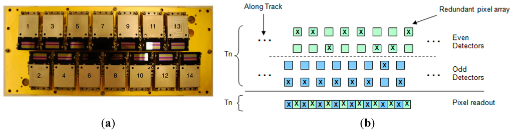
Figure 1.
(a) OLI focal plane array, showing focal plane module (FPM)-level staggering [5]; (b) example of even-odd detector staggering within a VNIR band in an FPM [4]
The OLI has three on-board radiometric calibration devices—lamps, a shutter and solar diffuser panels [6]. For this paper, the solar diffuser panels are the most important to consider. The OLI contains two different space-grade Spectralon® diffuser panels for radiometric characterization. They work by reflecting sunlight from the solar port of the OLI into the telescope. The first panel, known as the “working” panel, is deployed about every eight days to characterize OLI’s detectors. The second panel, known as the “pristine” panel, is deployed approximately bi-yearly to track changes in the working panel due to UV degradation from solar exposure [5].
2. Review of Earth Imagery-Based Relative Calibration Methods
Much work has gone into the successful development of vicarious methods for flat-fielding satellite imagery [7,8,9,10]. These methods are especially necessary for those satellite instruments that carry no on-board calibrators. In this section, an optimized version of the side-slither maneuver for OLI is presented. In addition, the background for a new method based on the use of deep convective clouds (DCCs) is also established.
2.1. Side-Slither Maneuver
With the emergence of pushbroom imaging, the side-slither maneuver has become an attractive solution for relative calibration. In a linear pushbroom array, an image is formed one row (frame) at a time as the array is “pushed” along the velocity vector. A side-slither maneuver rotates the array 90 degrees on its yaw axis, meaning that every detector is aligned to image the same target as it moves along the velocity vector [7]. However, when considering this maneuver for instruments like OLI with detector-level staggering, there are some key differences to note. First, since the FPMs are staggered within the focal array, the even and odd FPMs will image along disjoint paths in side-slither mode. Second, detectors within an FPM are also staggered. Refer to Figure 2 for an illustration of the side-slither maneuver over a staggered detector set over a target. Thus, in a side-slither maneuver with ideal focal plane alignment, there are four unique image paths at the detector level. However, perfect alignment of FPMs over a “uniform” target is impractical to expect, so corrective measures should be considered within even/odd detector sets at the FPM level.
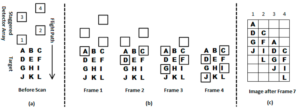
Figure 2.
(a) Setup of a yawed, staggered detector array about to scan a target; (b) execution of the side-slither maneuver over the target; (c) image of the collect.
Note that Figure 2 provides a very simplified view of the maneuver using one FPM, neglecting several practical design (e.g., optical distortions, detector look angles) and execution (e.g., Earth rotation, atmospheric path, use of backup detectors) considerations for the sake of clearly illustrating how the collect data is gathered.
Target selection is a key component for accurate side-slither characterization. As with other Earth imagery-based calibration methods, target spatial uniformity is a must. Assuming detector response linearity, the spectral radiance of a site should be maximized to allow for characterization with the best possible signal-to-noise ratio. For polar regions in particular, this occurs when the Sun elevation angle is maximized. For the VNIR bands on OLI, side-slither sites with the highest spectral radiance are those over snow-covered arctic regions, such as Greenland and Dome C of Antarctica. For SWIR wavelengths, Saharan desert sites provide high enough spectral radiance for accurate characterization. One advantage of using this method over spatially-uniform regions is that it produces very flat fields for optimal analysis [2,7]. The notable disadvantages of side-slither are that: (1) the maneuver must be carried out in place of normal Earth imaging, meaning a loss of valuable data depending on the region imaged; and (2) the “uniform” sites used are not really spatially uniform and, so, add additionally variability to detector relative gain estimates.
2.2. Lifetime Image Statistics
Another approach for the detector-level characterization of pushbroom sensors involves gathering statistics from multiple images over the course of the sensor’s life span. This is also known as the lifetime statistics approach. In this method, each detector output is represented as an independent random variable. Given enough samples, it is reasonable to assume that each detector has viewed roughly the same radiance field in a statistical sense across segments of the focal plane where view angle variation is small, e.g., within an FPM. This approach was first developed to calibrate OLI’s experimental predecessor on-board the EO-1 satellite: the Advanced Land Imager (ALI) [8]. Basic statistics were calculated for each detector in each scene by the ALI Image Assessment System (ALIAS) and stored in a characterization database. Similarly, whenever a Landsat 8 Earth scene is processed through the Level 1 Product Generation System (LPGS), image statistics are calculated and stored in the Landsat 8 radiometric characterization database, readily allowing the implementation of calibration methods based on lifetime statistics. Initially, all available data were used to characterize relative gains [8], but as more data were collected, the approach was refined to use subsets of lifetime data based on date range, image mean and image standard deviation. Results from this approach have shown that relative gains derived from around 400 binned high mean, high standard deviation images provide acceptable corrective results [9,10]. Since only 400 binned scenes were required for gain estimates to converge, one advantage of using this method is that it allowed for frequent relative gain characterization, providing valuable insight into how fast detectors are degrading. The main disadvantage of this method for an instrument like OLI is the sheer amount of data being stored. With almost 70,000 detectors to characterize and 675 Earth images collected daily, querying for scene statistics can take considerable time.
3. Methodology
This section details the radiometric characterization procedure used for each method. Assuming linear detector response, the initial quantized radiance from a detector can be expressed as:
where Lλ is the true spectral radiance measured by the detector, B is the digital count due to electronic bias and G is the product of relative and absolute gain coefficients to correct for detector-level non-uniformity and convert counts to spectral radiance, respectively. Since this paper solely focuses on relative correction within an FPM, (1) can instead be considered as:
where grel is the detector’s gain relative to the mean in the FPM and is the digital representation of the “true” radiance measured by the detector.
After Earth data are collected for Landsat 8, they are downlinked to a ground station and undergo some minor corrections and reformatting into an L0Ra (Level 0 Reflectance a) product [4]. This product is then sent through the Landsat 8 Image Assessment System (IAS), where it is radiometrically and geometrically processed into a finished data product. A brief overview of IAS radiometric processing steps begins with the characterization of certain artifacts (dropped frames, impulse noise, saturated pixels), then electronic bias determination and removal and detector response linearization before gain application (relative and absolute) and data conversion from electronic counts to reflectance. At this point, the data is a Level 1 Reflectance (L1R) product. For a full description of the individual IAS algorithms, see [11]. For the work done in this paper, there are two benefits to utilizing the IAS. First, each processing algorithm can be toggled, allowing the user to process scenes or calibration collects to a certain, predefined point. This is particularly useful for the side-slither data, which can be radiometrically processed to the point where relative gains can be characterized. Second, custom calibration parameter files (CPFs) can be specified for each work order, making the IAS an ideal tool for evaluating relative gain performance.
3.1. Side-Slither
To estimate relative gains for OLI from side-slither data, the data need to be radiometrically processed (bias removed, response linearized) before gains can be derived. This is done using the IAS, as mentioned above. As detailed below, for each FPM in each band, the data are then adjusted to align samples taken over the same target, suitable flat-field data are selected and then the gains are derived after compensating for even/odd detector alignment within the FPM. Using suitable flat-field regions of data, a relative gain coefficient for the i-th detector in a set j frames long is derived using first-order statistical data from the selected flat-field region,
where and denote the i-th detector mean and the FPM flat-field image mean, respectively. If no flat-field region meets selection criteria, then no relative gains are derived for that band.
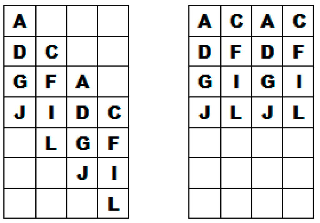
Figure 3.
Side-slither collect before and after frame shift correction. Note how even/odd start frames are lined up.
3.1.1. Frame Shift Correction
As demonstrated in Figure 2, each detector set within an FPM will image the same target over the course of the collect. Due to temporal lag, the same target viewed by each detector in even/odd sets is shifted two frames up or down, depending on the yaw direction, from its set neighbor, as shown in Figure 2c. Thus, to line up detector sets in a target sense rather than a temporal one, each successive detector’s data are shifted two more frames up/down than its predecessor. An alternate solution that lines up set target frames and start frames between even/odd sets is to shift the successive detector’s data in the FPM one additional frame up/down. Refer to Figure 3 for an illustration of the latter.
3.1.2. Flat-Field Data Selection
Due to interval coverage beyond the intended uniform target and clouds, the entirety of a side-slither collect (up to several hundred kilometers) is not uniform enough to use as a flat-field. Thus, the appropriate flat-field data regions need to be selected for each even/odd detector set for every band and FPM if they exist. Since this needs to be done for over 200 unique sets for each side-slither collect (8 bands, 14 FPMs/band and even/odd detectors), an automated selection approach is necessary.
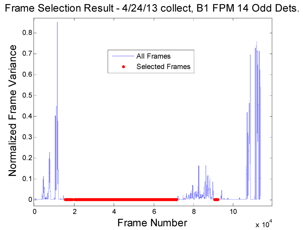
Figure 4.
Example of frame selection algorithm output.
The method developed for flat-field data selection involves thresholding and analyzing the rate of change of each frame’s index of dispersion (ratio of variance to the mean for a set of data). Thus, the following procedure is used to find sufficient flat-fields in each unique set of side-slither data:
- (1)
- After frame shift correction, the squared coefficient of variation (SCV) is calculated for each frame. This provides a basis for inter-frame comparison.
- (2)
- The SCVs are run through a length-101 maximum filter to put more of a buffer between uniform and non-uniform regions in the base data.
- (3)
- To ensure estimate integrity, the minimum number of contiguous frames for multispectral bands is set to 1000. Slight errors in detector alignment can be compensated for by ensuring that a large region (>10 km) of imagery is obtained, and this is also necessary for even/odd detector normalization. For Band 8, to cover the same ground as the multispectral bands, the minimum is 2000.
- (4)
- First thresholding attempt: Select indices of all continuous regions of at least the minimum length where the absolute difference between SCVs is less than or equal to 0.0001. This value was selected to be an order of magnitude better than the streaking threshold necessary to ensure that no images stripes can be observed visually.
- (5)
- If no regions are selected in the first attempt and the mean absolute difference between SCVs is greater than the first threshold, try Step 4 again using the mean absolute difference between SCVs as the threshold. If no regions are selected after the second threshold (i.e., Step 5), then relative gains are not derived for this band.
The frame indices selected using the above filtering contain sufficiently flat regions for relative gain derivation, should they exist. Figure 4 provides a visual example of the frame selection algorithm.
3.1.3. Even/Odd Detector Artifact Removal
Since even/odd detector staggering results in two disjoint datasets per FPM, even and odd detector relative gains should typically be derived separately. This results in the mean of each individual set equaling one. However, the mean for the combined sets of detectors should also be one, meaning that individual even/odd sets are not necessarily equal to one when derived together. If the set means are different, this will become apparent in the form of even/odd streaking when the gains are applied to an image. Thus, even and odd detector relative gain sets for each FPM require some form of normalization, so that they do not introduce additional artifacts into the imagery. This can be done using the side-slither data itself. Intuitively, even and odd sets for each FPM are unique, so one would expect at-sensor radiance to differ enough between them to prohibit comparison. However, since sites for the side-slither maneuver are specifically selected for their radiometric and spatial uniformity, it is reasonable to assume that at-sensor radiance (at least in a statistical sense over large regions) for each set is equal. Thanks to the second frame shift correction method established above, a viable frame-by-frame comparison of common even/odd detector flat-fields is possible using the procedure below:
- (1)
- Using the output from the flat-field selection algorithm, select common flat-field frames between even/odd sets.
- (2)
- Calculate the frame means for even/odd sets
- (3)
- Normalize each set of means to the overall (even and odd combined) mean. This accounts for differences in radiance due solely to even/odd detector characteristics.
- (4)
- Use a two-sample Kolmogorov–Smirnov test on the two detector mean sets to determine if they are similarly distributed with the following hypotheses at the 95% level:Ho: Even/odd detector sets are sampled from the same population and should be considered together;Ha: Even/odd detectors should not be considered as one set.
If the null hypothesis is upheld, then relative gains are derived using the combined even/odd flat-field data; no extra normalization is necessary. If the null hypothesis is rejected, then the relative gains are derived as two separate sets, requiring normalization through an alternative method.
3.2. DCC Image Statistics for the Cirrus Band
The cirrus band on OLI provides a special challenge for Earth imagery-based relative calibration techniques, since virtually no ground signal in this band is transmitted through the atmosphere. As a result, side-slither data for this band contains a very small signal and the cumulative scene statistics are too heavily weighted at the low-signal end using the same binning techniques as other bands. One possible solution is to bin scenes containing deep convective clouds (DCCs). DCCs are very cold and highly reflective clouds, extending into the tropopause layer of the atmosphere and reaching heights of 14–19 km. At this height, the effect of atmospheric water vapor absorption is minimal. At a small Sun zenith angle (less than 30°), DCCs can be considered as an isotropic, near-Lambertian solar reflector. Previously, Doelling et al. have shown that DCCs are ideal absolute visible band calibration targets with a high signal-to-noise ratio and easy to identify using an infrared threshold [12,13]. If only DCC image statistics are considered, then a lifetime statistics approach is applicable for calibrating OLI’s cirrus band.
Finding DCC scenes in the OLI image archive was done making use of several thresholds utilizing scene statistics stored in the Landsat 8 radiometric characterization database during LPGS processing. Starting with the criteria mentioned in [12] and [13], a list of conditions was refined for the selection of scenes in the characterization database with the most DCC coverage. A scene was selected for use if it met each of the criteria below.
- (1)
- The scene is between ±30° latitude;
- (2)
- The solar zenith angle for the scene is less than 30°;
- (3)
- In the red band, the scene mean radiance is greater than 220 W/m2/sr/µm;
- (4)
- In the cirrus band, the scene mean radiance is greater than 10 W/m2/sr/µm;
- (5)
- In the first TIRS band (Band 10 in Landsat 8 imagery), the scene mean brightness temperature is less than 220 K.
For scenes meeting the criteria, detector means and scene means were extracted from the radiometric characterization database. Relative gains were then derived on an FPM level, using a method very similar to criterion (3), but instead utilizing means from the characterization database rather than calculating them individually.
4. Results and Analysis
Since the methods in this paper are backups to on-board diffuser-based relative gain characterization, comparing the performance of secondary methods with the primary one is paramount. Because the foremost goal of relative gain calibration is to eradicate detector-to-detector non-uniformity (streaking), a streaking metric will be used as a primary means for comparison. In a uniform L1R data product, a detector is compared to its immediate neighbors using the equation:
where is the mean digital count of the i-th detector over every frame. For edge detectors in each FPM, only the immediate neighbor is considered. For reference, note that a streaking metric around 0.25% is roughly where streaks become visibly apparent in homogeneous unaltered imagery. Note that although the streaking metric helps explain high-frequency differences between diffuser and side-slither gains, lower frequency differences could be present and, thus, avoid explanation with this metric.
4.1. Side-Slither
At the time this paper was written, there were 19 total side-slither collects available to analyze. Thirteen of these were suitable for OLI relative gain characterization. Out of these, 11 complete sets of relative gains were derived for analysis. Table 2 provides a breakdown of the side-slither collects used in this paper. Intervals were collected over Egypt (EGY), Libya (LBY), Niger (NER), Greenland (GRL) and Antarctica (ATA).
Table 2.
List of side-slither collects analyzed with WRS-2 path/row coverage.
| Date of Collect | Location | Path | Rows |
|---|---|---|---|
| 3-26-2013 | Niger | 189 | 45–48 |
| 4-5-2013 | Libya/Niger | 187 | 38–49 |
| 4-20-2013 | Egypt | 177 | 36–47 |
| 4-24-2013 | Greenland | 4 | 3–22 |
| 5-6-2013 | Egypt | 177 | 33–47 |
| 5-12-2013 | Greenland | 2 | 4–25 |
| 7-13-2013 | Greenland | 4 | 5–21 |
| 11-30-2013 | Antarctica | 88 | 103–117 |
| 12-16-2013 | Antarctica | 88 | 103–117 |
| 1-1-2014 | Antarctica | 88 | 103–117 |
| 4-11-2014 | Niger | 189 | 44–51 |
To accurately characterize streaking and to compare to diffuser-based relative gain correction, the relative gains were applied to spatially-uniform imagery and compared. The bands that exhibit the most detector non-uniformity are the coastal/aerosol and the SWIRs, so analysis hereafter will primarily focus on these bands.
Because there is no single optimal site for every spectral band in OLI, two different sites were utilized—Greenland, at WRS-2 Path/Row 11/7 for the VNIR/PAN bands, and Niger, at WRS-2 Path/Row 188/46 for the SWIR bands. Because the former is so uniform, streaking artifacts in the visible bands are apparent without any linear stretching. Finding suitable images to test the SWIR bands is more of a challenge, since high-radiance scenes in these bands are over regions that are not as spatially uniform, but some exist within the Sahara Desert. To get an initial sense of how side-slither relative gains visually perform compared to diffuser-based gains, a Greenland scene from 16 June 2013, was processed using the most current diffuser-based gains for the quarter this scene was acquired and gains from three side-slither collects near this scene acquisition date. In addition to evaluating side-slither relative gains, this visual comparison could suggest that operational relative gain parameters might need more frequent updating. Currently, the diffuser gains for each quarter are calculated by averaging estimates from each “working” diffuser collect that occurred during that quarter. The only changes in IAS processing between the four test sets are the relative gains in the CPFs for each work order. Figure 5 shows an example of how side-slither relative gains can aid in streaking reduction.
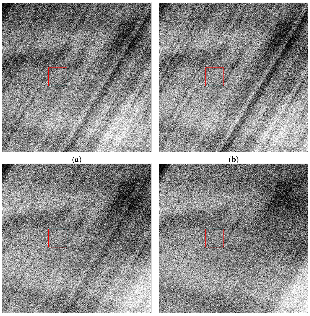
Figure 5.
Hard-stretched test image (WRS-2 11/7, 16 June 2013) of the coastal/aerosol band, zoomed in around FPM 8 with the following sets of relative gains applied: (a) diffuser-based; (b) first side-slither (3/26/13, Niger (NER)); (c) fourth side-slither (4/24/2013, Greenland (GRL)); (d) sixth side-slither (5/12/13, GRL).
To determine whether or not the relative gains are changing over time, a simple exercise was conducted: all complete sets of side-slither relative gains were applied to three images of the same Greenland site—on 16 June 2013, 16 September 2013, and 1 April 2014. Table 3 shows the mean streaking metric percentages for the complete set of side-slither relative gains across the three images. For comparison, the diffuser-based relative gains were also applied.
Table 3.
Mean streaking metric percentages for the 11/7 site acquired on the following dates: (a) 16 June 2013; (b) 16 September 2013; (c) 1 April 2014. Gray highlighting denotes collects closest to test image acquisition. Bolded numbers mark performance that is superior to the default processing parameters. CPF, calibration parameter file.
| Band | CPF | 3/26/13 (NER) | 4/5/13 (LBY) | 4/20/13 (EGY) | 4/24/13 (GRL) | 5/6/13 (EGY) | 5/12/13 (GRL) | 7/13/13 (GRL) | 11/30/13 (ATA) | 12/16/13 (ATA) | 1/1/14 (ATA) | 4/11/14 (NER) |
|---|---|---|---|---|---|---|---|---|---|---|---|---|
| C/A | 0.027 | 0.039 | 0.032 | 0.028 | 0.021 | 0.027 | 0.017 | 0.009 | 0.051 | 0.027 | 0.030 | 0.035 |
| Blue | 0.022 | 0.023 | 0.026 | 0.022 | 0.012 | 0.018 | 0.016 | 0.010 | 0.051 | 0.022 | 0.022 | 0.023 |
| Green | 0.012 | 0.017 | 0.016 | 0.026 | 0.008 | 0.044 | 0.007 | 0.006 | 0.028 | 0.012 | 0.012 | 0.017 |
| Red | 0.007 | 0.012 | 0.017 | 0.038 | 0.007 | 0.040 | 0.006 | 0.005 | 0.012 | 0.009 | 0.009 | 0.014 |
| NIR | 0.005 | 0.010 | 0.021 | 0.042 | 0.007 | 0.043 | 0.009 | 0.006 | 0.011 | 0.009 | 0.010 | 0.014 |
| PAN | 0.075 | 0.098 | 0.099 | 0.097 | 0.083 | 0.101 | 0.087 | 0.077 | 0.069 | 0.084 | 0.095 | 0.102 |
(a)
| Band | CPF | 3/26/13 (NER) | 4/5/13 (LBY) | 4/20/13 (EGY) | 4/24/13 (GRL) | 5/6/13 (EGY) | 5/12/13 (GRL) | 7/13/13 (GRL) | 11/30/13 (ATA) | 12/16/13 (ATA) | 1/1/14 (ATA) | 4/11/14 (NER) |
|---|---|---|---|---|---|---|---|---|---|---|---|---|
| C/A | 0.034 | 0.054 | 0.047 | 0.039 | 0.040 | 0.037 | 0.033 | 0.017 | 0.040 | 0.016 | 0.017 | 0.022 |
| Blue | 0.021 | 0.033 | 0.034 | 0.029 | 0.023 | 0.024 | 0.019 | 0.011 | 0.043 | 0.015 | 0.014 | 0.022 |
| Green | 0.010 | 0.024 | 0.022 | 0.027 | 0.016 | 0.046 | 0.012 | 0.011 | 0.022 | 0.011 | 0.012 | 0.019 |
| Red | 0.009 | 0.015 | 0.018 | 0.038 | 0.012 | 0.041 | 0.010 | 0.010 | 0.012 | 0.011 | 0.012 | 0.014 |
| NIR | 0.008 | 0.013 | 0.023 | 0.042 | 0.011 | 0.043 | 0.013 | 0.010 | 0.013 | 0.012 | 0.013 | 0.017 |
| PAN | 0.015 | 0.028 | 0.029 | 0.039 | 0.018 | 0.036 | 0.019 | 0.016 | 0.023 | 0.018 | 0.018 | 0.033 |
(b)
| Band | CPF | 3/26/13 (NER) | 4/5/13 (LBY) | 4/20/13 (EGY) | 4/24/13 (GRL) | 5/6/13 (EGY) | 5/12/13 (GRL) | 7/13/13 (GRL) | 11/30/13 (ATA) | 12/16/13 (ATA) | 1/1/14 (ATA) | 4/11/14 (NER) |
|---|---|---|---|---|---|---|---|---|---|---|---|---|
| C/A | 0.025 | 0.064 | 0.057 | 0.050 | 0.049 | 0.047 | 0.042 | 0.026 | 0.041 | 0.013 | 0.013 | 0.018 |
| Blue | 0.032 | 0.040 | 0.042 | 0.036 | 0.029 | 0.030 | 0.020 | 0.015 | 0.037 | 0.009 | 0.010 | 0.024 |
| Green | 0.017 | 0.025 | 0.025 | 0.030 | 0.018 | 0.049 | 0.013 | 0.011 | 0.020 | 0.007 | 0.007 | 0.015 |
| Red | 0.006 | 0.015 | 0.018 | 0.039 | 0.010 | 0.042 | 0.009 | 0.007 | 0.009 | 0.007 | 0.007 | 0.013 |
| NIR | 0.006 | 0.010 | 0.022 | 0.041 | 0.007 | 0.043 | 0.010 | 0.006 | 0.010 | 0.009 | 0.009 | 0.013 |
| PAN | 0.019 | 0.032 | 0.033 | 0.041 | 0.016 | 0.039 | 0.015 | 0.013 | 0.017 | 0.010 | 0.010 | 0.033 |
(c)
Table 3 shows that gains derived from side-slither collects closer to the image acquisition date indeed provide the most streaking improvement in the time series. In several cases, relative gains from side-slither collects over polar regions reduce visible band streaking more than current processing parameters. Although the diffuser-based gains showed the best streaking improvement in the red and NIR bands, side-slither gains still corrected streaking to within 0.005% of them. In typical Earth imagery, this means the difference in streaking reduction between sets will not be visually apparent. The relative gains applied to the Niger test set over three similarly different dates resulted in similar conclusions: gains derived from desert-based side-slither collects close to test image acquisition dates (particularly Niger and Libya) correct streaking to within 0.01% of current processing parameters. Since relative gains from side-slithers closer to the test image date consistently perform better, it appears that detector relative gains are changing over time. To gain a clearer sense of how fast relative gains are changing over time, the differences between the first set of side-slither relative gains with each subsequent set was calculated for each band and plotted. Due to the large temporal gap between some gain sets, they are plotted in the order they were collected, starting from the bottom, as shown in Figure 6.
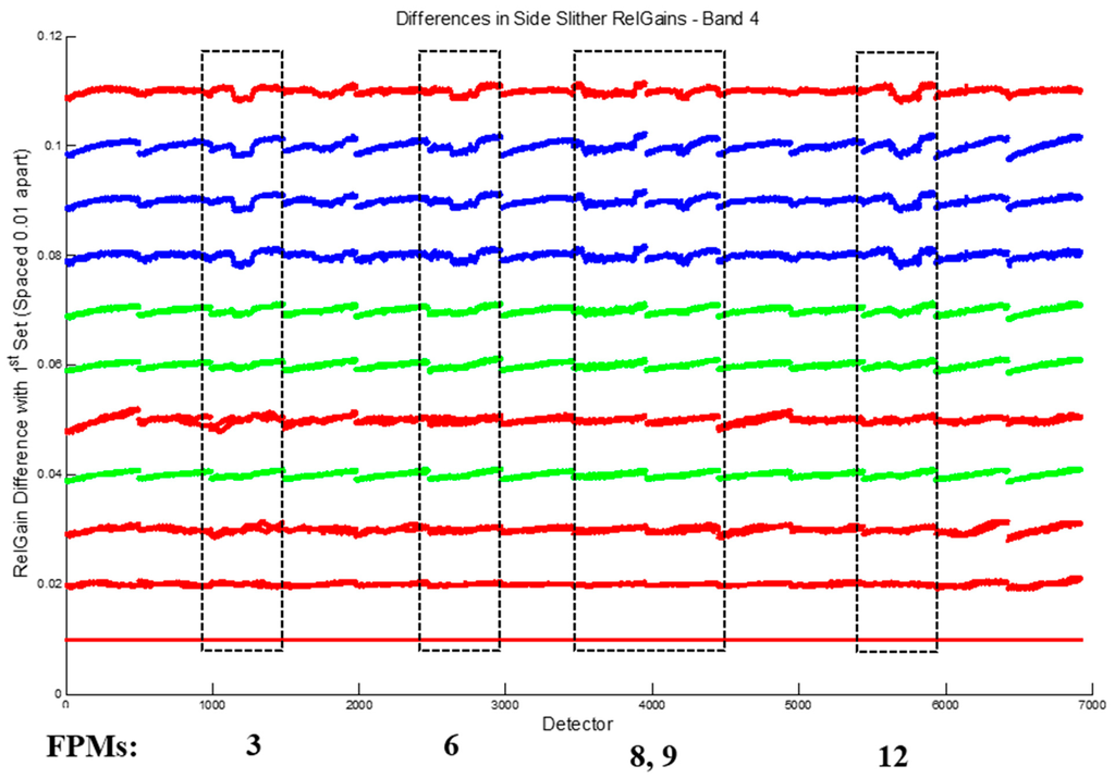
Figure 6.
Temporal differences between side-slither relative gains in the red band using the first set as a basis. Note that each collect is color-coded by the region slithered: red for desert, green for Greenland and blue for Antarctica. Boxed FPMs are numbered below the plot.
Figure 6 shows a clear emergence of differences of up to 0.23% in side-slither relative gains (referred to as RelGains in the plot title) over time for the red band in FPMs 3, 6, 8, 9 and 12. Other visible bands showed similar change traceability, which is consistent with the temporal changes shown in solar collect data [14]. While some differences exist over time for the SWIR bands, they are harder to discern in temporal plots due to substantial signal-level differences between collects. Thus, these temporal differences were quantitatively assessed for further clarity. Table 4 shows the maximum detector relative gain percent difference between first side-slither collect and each successive collect.
Table 4 shows that every spectral band has detectors that are drifting, some as much as 0.47% over the course of a year. The coastal/aerosol band, whose differences do not appear dependent on collect signal level, shows the most drift over time. In the SWIR bands, detectors are drifting as much as 0.38% over a year. Note that when considering SWIR detector drift, the relative gain differences from the Arctic/Antarctic sites are excluded, since those percent differences are due to the low signal level. Although the VNIR bands are most accurately characterized using side-slithers over polar regions, the gains derived for these bands over desert regions are useful for continuous tracking of detector drift.
Table 4.
Maximum relative gain percent differences obtained from side-slither collects as a function of time during the first year of OLI operation.
| Band | 3/26/13 (NER) | 4/5/13 (LBY) | 4/20/13 (EGY) | 4/24/13 (GRL) | 5/6/13 (EGY) | 5/12/13 (GRL) | 7/13/13 (GRL) | 11/30/13 (ATA) | 12/16/13 (ATA) | 1/1/14 (ATA) | 4/11/14 (NER) |
|---|---|---|---|---|---|---|---|---|---|---|---|
| C/A | - | 0.09 | 0.24 | 0.15 | 0.29 | 0.22 | 0.25 | 0.46 | 0.42 | 0.47 | 0.44 |
| Blue | - | 0.12 | 0.16 | 0.16 | 0.29 | 0.2 | 0.19 | 0.27 | 0.21 | 0.25 | 0.2 |
| Green | - | 0.08 | 0.15 | 0.11 | 0.17 | 0.12 | 0.14 | 0.22 | 0.21 | 0.23 | 0.16 |
| Red | - | 0.12 | 0.14 | 0.12 | 0.21 | 0.14 | 0.13 | 0.18 | 0.19 | 0.23 | 0.15 |
| NIR | - | 0.13 | 0.2 | 0.13 | 0.2 | 0.13 | 0.14 | 0.13 | 0.16 | 0.23 | 0.1 |
| SWIR1 | - | 0.22 | 0.21 | 0.88 | 0.26 | 0.68 | 1.16 | 1.39 | 1.06 | 1.19 | 0.38 |
| SWIR2 | - | 0.24 | 0.22 | 0.72 | 0.25 | 0.68 | 0.75 | 0.63 | 0.68 | 1.24 | 0.24 |
| PAN | - | 0.11 | 0.17 | 0.17 | 0.27 | 0.2 | 0.18 | 0.22 | 0.22 | 0.26 | 0.22 |
4.2. DCC Image Statistics for Cirrus Band
Due to the scarcity of DCC scenes meeting the selection criteria, the time frame for the images queried was from May 2013, to October 2013, crossing over three different quarters. As a result, statistics from 69 DCC scenes were used for gain derivation. To assess the effectiveness of these gains in streaking reduction, they were applied to several DCC test scenes—part of the derivation collection and not—and compared to the performance of diffuser-based relative gains using the scene-based streaking metric defined earlier. Results were similar on all test scenes, and a representative example is given here. Figure 7 shows a visual comparison between gain sets on a DCC scene. This particular test scene is part of the collection used to derive the relative gains. Note that the zoomed portion of Figure 7b shows notable streaking improvement over that apparent in Figure 7a. FPM boundaries are clearly present in the full image in Figure 7b, since the DCC relative gains were derived only on an FPM level. For a quantification of streaking in both test images, refer to Figure 8. Figure 8 shows that streaking is generally lower across the scene when corrected with DCC relative gains. The streaking metric for the DCC relative gain corrected scene did not go above 0.4% and had many fewer detectors above 0.2% as compared to the CPF gains. Although the test scene was by no means uniform, use of the streaking metric provides some form of quantitative performance evaluation for relative gains for this band.
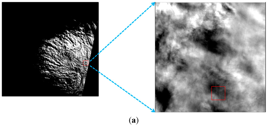
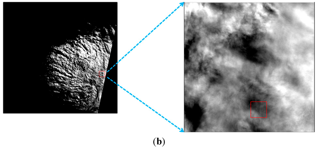
Figure 7.
Hard-stretched test image for the cirrus band (WRS-2 12/55, 19 June 2013) zoomed in on FPM 14 with the following relative gains applied: (a) diffuser-based; (b) deep convective cloud (DCC)-based.
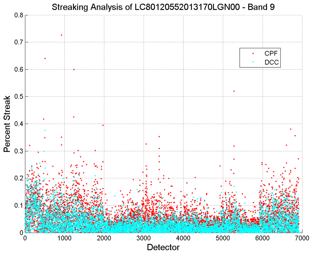
Figure 8.
Streaking analysis of the DCC test image shown in Figure 7.
5. Conclusions
Side-slither maneuvers that rotate a satellite such that linear arrays of detectors are aligned with the velocity vector have been successfully used for several years as a mechanism for measuring differences in gains between detectors in the array. This approach has been implemented with the Landsat 8 OLI sensor that has 12 bits of radiometric resolution and an exceptionally high signal-to-noise ratio. These two factors significantly increase the precision necessary for the side-slither maneuver to estimate relative detector gains in order to ensure no visual streaking or striping exists in imagery collected by the instrument. To achieve an acceptable performance level with the OLI, an improved method of characterizing detector non-uniformity from side-slither data was implemented that exhibits performance at a level that is comparable to the standard diffuser-based calibration, which is currently employed with the instrument. Improvements included an algorithm to ensure that optimal regions of the side-slither image collect were used to estimate relative gains, the identification of optimal locations for each spectral band (i.e., Arctic and Antarctic regions for short wavelength bands and desert regions for the NIR and SWIR bands) and a simplified even/odd detector gain estimation. These improvements have demonstrated performance that can allow continued updating of relative gains, even if the primary methodology using on-board diffuser panels fails.
Studies over the first year of OLI operation have indicated that the values for the relative gains of the detectors are changing as a function of time. This was observed in the imagery itself, but was also quantified using the side-slither estimates of detector gain. As a result, these changes are now trackable, and it is possible to provide continuous relative gain updates that can minimize striping and streaking in imagery obtained from all time periods over the lifetime of the satellite.
Lastly, a novel approach was developed to estimate relative gains of bands at wavelengths where Earth surface imagery is unavailable, such as the cirrus band on OLI. The method is based on the use of multiple DCC scenes from which statistical comparisons of detector responses can be drawn to estimate relative gain. Results of this methodology are also comparable to on-board methods and provide an excellent backup in the case of the failure or degradation of those approaches.
Acknowledgments
The authors thank the Landsat Calibration/Validation Team at the USGS Earth Resource Ovservation and Science (EROS) Center and NASA Goddard Space Flight Center for their advice and feedback on this project. The authors also thank Jordan Ulmer of the South Dakota State University Image Processing Lab for generating a list of validation test images. This work was supported by NASA Grant NNX09AH23A from the Landsat Project Science Office, by USGS EROS Grant G08AC00031 and also in part by the South Dakota Space Grant Consortium.
Author Contributions
Frank Pesta and Suman Bhatta are graduate research assistants in the Image Processing Laboratory at South Dakota State University, supervised by Dennis Helder and Nischal Mishra. Frank Pesta developed and refined the side-slither methodology presented. Suman Bhatta developed the DCC approach for relative calibration.
Conflicts of Interest
The authors declare no conflict of interest.
References
- Adriansen, S.; Benhadj, I.; Duhoux, G.; Dierckx, W.; Dries, J.; Heyns, W.; Kleihorst, R.; Livens, S.; Nackaerts, K.; Reusen, I.; et al. Building a calibration and validation system for the PROBA-V satellite mission. In Proceedings of the ISPRS XXXVIII International Calibration and Orientation Workshop, Castelldefels, Spain, 10–12 February 2010.
- Anderson, C.; Naughton, D.; Brunn, A.; Thiele, M. Radiometric correction of RapidEye imagery using the on-orbit side-slither method. Proc. SPIE 2011. [Google Scholar] [CrossRef]
- Operational Land Imager (OLI) Landsat Science. Available online: http://landsat.gsfc.nasa.gov/?p=5447 (accessed on 26 June 2014).
- Landsat 8 Mission Data Format Control Book. Available online: http://landsat.usgs.gov/documents/LDCM-DFCB-004.pdf (accessed on 26 June 2014).
- Markham, B.L.; Barsi, J.A.; Kvaran, G.; Ong, L.; Kaita, E.; Biggar, S.; Czapla-Myers, J.; Mishra, N.; Helder, D.L. Landsat-8 operational land imager radiometric calibration and stability. Remote Sens. 2014, in press. [Google Scholar]
- Knight, E.J.; Kvaran, G. Landsat-8 operational land imager design, characterization, and performance. Remote Sens. 2014, in press. [Google Scholar]
- Henderson, B.G.; Krause, K.S. Relative radiometric correction of QuickBird imagery using the side-slither technique on-orbit. Proc. SPIE 2004. [Google Scholar] [CrossRef]
- Angal, A; Helder, D.L. Advanced land imager relative gain characterization and correction. In Proceedings of Pecora 16—Global Priorities in Land Remote Sensing, Sioux Falls, SD, USA, 25 October 2005.
- Shrestha, A.K. Relative Gain Characterization and Correction for Pushbroom Sensors Based on Lifetime Image Statistics and Wavelet Filtering. Master’s Thesis, South Dakota State University, Brookings, SD, USA, 2010. [Google Scholar]
- Shrestha, A.K.; Helder, D.L.; Anderson, C. Relative gain characterization and correction for pushbroom sensors based on lifetime image statistics. In Proceedings of the Civil Commercial Imagery Evaluation Workshop, Fairfax, VA, USA, 17 March 2010.
- Landsat 8 Cal/Val Algorithm Description Document. Available online: http://landsat.usgs.gov/documents/LDCM_CVT_ADD.pdf (accessed on 26 June 2014).
- Doelling, D.R.; Morstad, D.; Scarino, B.R.; Bhatt, R.; Gopalan, A. The characterization of deep convective clouds as an invariant calibration target and as a visible calibration technique. IEEE Trans. Geosci. Remote Sens. 2013, 51, 1147–1159. [Google Scholar] [CrossRef]
- Doelling, D.R.; Nguyen, L.; Minnis, P. On the use of deep convective clouds to calibrate AVHRR data. Proc. SPIE 2004. [Google Scholar] [CrossRef]
- Morfitt, R.; Markham, B.L.; Micijevic, E.; Scaramuzza, P.; Barsi, J.A.; Levy, R.; Ong, L.; Vanderwerff, K. OLI radiometric performance on-orbit. Remote Sens. 2014, in press. [Google Scholar]
© 2014 by the authors; licensee MDPI, Basel, Switzerland. This article is an open access article distributed under the terms and conditions of the Creative Commons Attribution license (http://creativecommons.org/licenses/by/4.0/).