1. Introduction
Lidar (light detection and ranging) or laser radar detects atmospheric parameters by transmitting laser pulse to the atmosphere and receiving the backscattering signals from molecules and aerosol particles, described by Rayleigh scattering and Mie scattering [
1]. Mie scattering is generally the most efficient of these scattering processes with cross-sections of the order 10
−26−10
−8 cm
2/particle, whereas Rayleigh cross-sections are in the region of 4.04 × 10
−27–7.24 × 10
−27 cm
2/molecule in the wavelength region from 490 nm to 565 nm [
2]. This Rayleigh cross-section follows a λ
−4 relation and, hence, shorter wavelengths exhibit greater scattering effects. Because of the extreme low backscattering cross section, lidar usually uses the high sensitive photon detector and photon counting technology to obtain the return signal from long distance by a long time accumulation [
3–
11]. Because of the strong solar background, the signal-to-noise ratio (SNR) of lidar during daytime could be greatly restricted, especially for the lidar operating at visible spectral region where solar background is prominent [
7]. A large number of background rejection techniques have been used to improve the SNR such as narrow band interference filter, Fabry-Perot etalon and field-of-view restriction, whereas the solar noise in superposition with the signal spectrum limits an effective margin for SNR improvement.
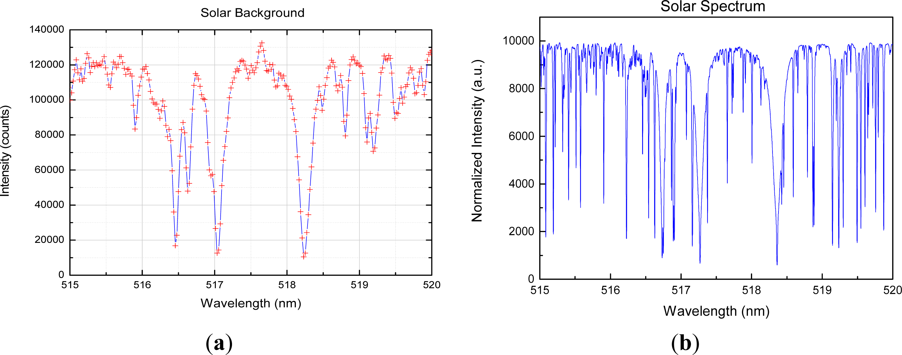
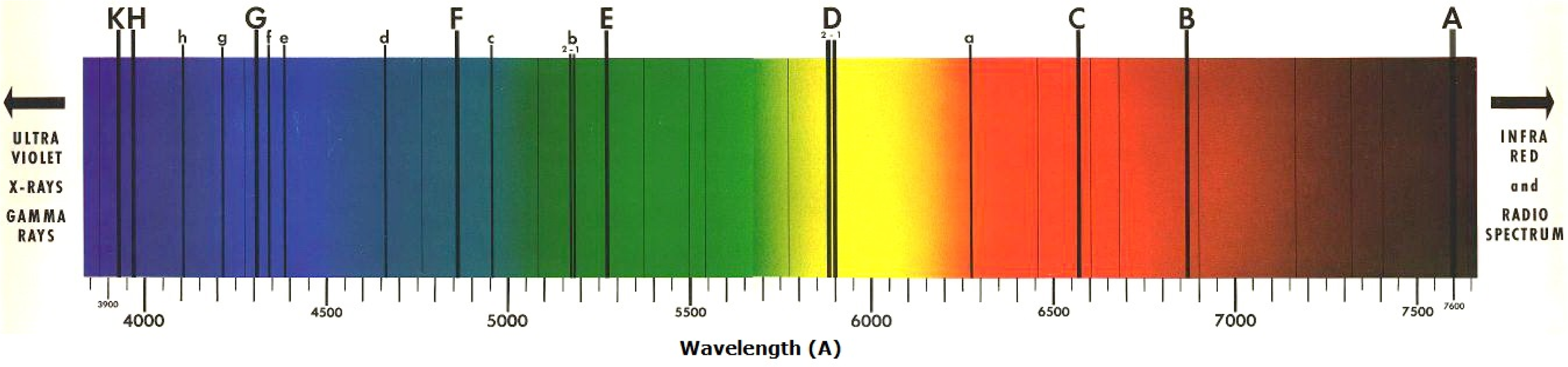
The absorption process of solar radiation is well known as the solar Fraunhofer spectra due to certain atmospheric constituent in either the solar atmosphere or that of the earth, first documented and mapped by Joseph von Fraunhofer in 1812. Because of the absorption process, the solar light reaching the earth’s surface exhibits certain “dark windows” rather than being a continuum of all wavelengths. Modern observations of solar spectrum can detect many thousands of lines. The wavelengths of the most notable lines for visible wavelengths [
12,
13] are given in
Figure 1. Fraunhofer lines produce strong absorptions and fingerprint information of sunlight. Therefore, those lines have been studied for free-space laser communications and passive optical sensing techniques [
14,
15]. A wavelength lying within a Fraunhofer line can carry optical communications with reduced interference from the solar background. The tunable source laser and the Fraunhofer filter were proposed to match the Doppler shifts of the source and background [
14]. A free-space Quantum key distribution system for Earth-space data link was described that lies within an H-alpha Fraunhofer line at 656.28 nm, to carry the signal with reduced interference from sunlight [
15]. Fraunhofer line radiometers were also suggested to identify certain materials of solar-stimulated luminescence [
16,
17]. A space mission called FLEX (Fluorescence Explorer) probe terrestrial vegetation by solar induced fluorescence that is detectable within the Fraunhofer lines in the red and blue-UV region [
18]. With regards to laser remote sensing, resonance fluorescence techniques have evolved to measure mesospheric metals such as Na, K, Fe, Ca, and Ca
+ are capable of measuring mesospheric metals densities in the middle atmosphere region 80–105 km [
19–
24]. The thermal broadening and Doppler frequency shift of the fluorescence spectrum of such metals have also been used to retrieve temperature and wind structures throughout the mesospheric region. These middle-atmosphere lidars spontaneously exhibit good signal-to-noise ratio during the daytime because the resonance fluorescence wavelengths of such metals are consistent with the strong Fraunhofer lines by the same metal atoms or ions in the solar atmosphere [
25]. This work describes a photon counting lidar prototype operating at the Fraunhofer lines in the green spectral region, the invisible spectral region of the solar spectrum, to achieve photon counting under intense solar background. The first criterion to select the dark lines is that the line has a strong absorption peak to minimize solar noise at the signal wavelength. The second criterion is that the line has broad linewidth to facilitate tuning of both the laser transmitter and optical filter. The last consideration is that the dark line is co-inside with some atomic or molecular absorption filter as potential high spectral resolution receiver. Based on the above criteria, it was found that three such lines exist, at 516.7327 nm, 517.2698 nm and 518.3619 nm, by the Magnesium atom in the solar chromospheres. The broadest linewidth of those is approximately 0.2 nm wide, slightly broader than that of tunable laser we have, 0.17 nm. Thus, optimization of the receiver optics such as high resolution monochromator/spectrograph is investigated to cover the margin to sufficiently minimize the solar noise such that equivalent photon counting efficiency in daytime can be obtained. The laser transmitter is an optical parametric oscillator pumped by 355 nm Nd:YAG (neodymium-doped yttrium aluminum garnet) laser and is tuned to the selected dark lines by which nearly 90% of solar radiation is absorbed. The prototype provides some theoretical references for optimized design of photon counting lidar in the visible spectral region with comparable SNR at night, which may contribute to the research on diurnal variation of the atmosphere and to the operational observation of lidar. The ongoing procedures included the application of atomic vapor filter as the receiver taking maximum heritages of traditional HSRL for wind, temperature and aerosol probing [
6–
10].
3. Solar Background Analysis for Selected Fraunhofer Line
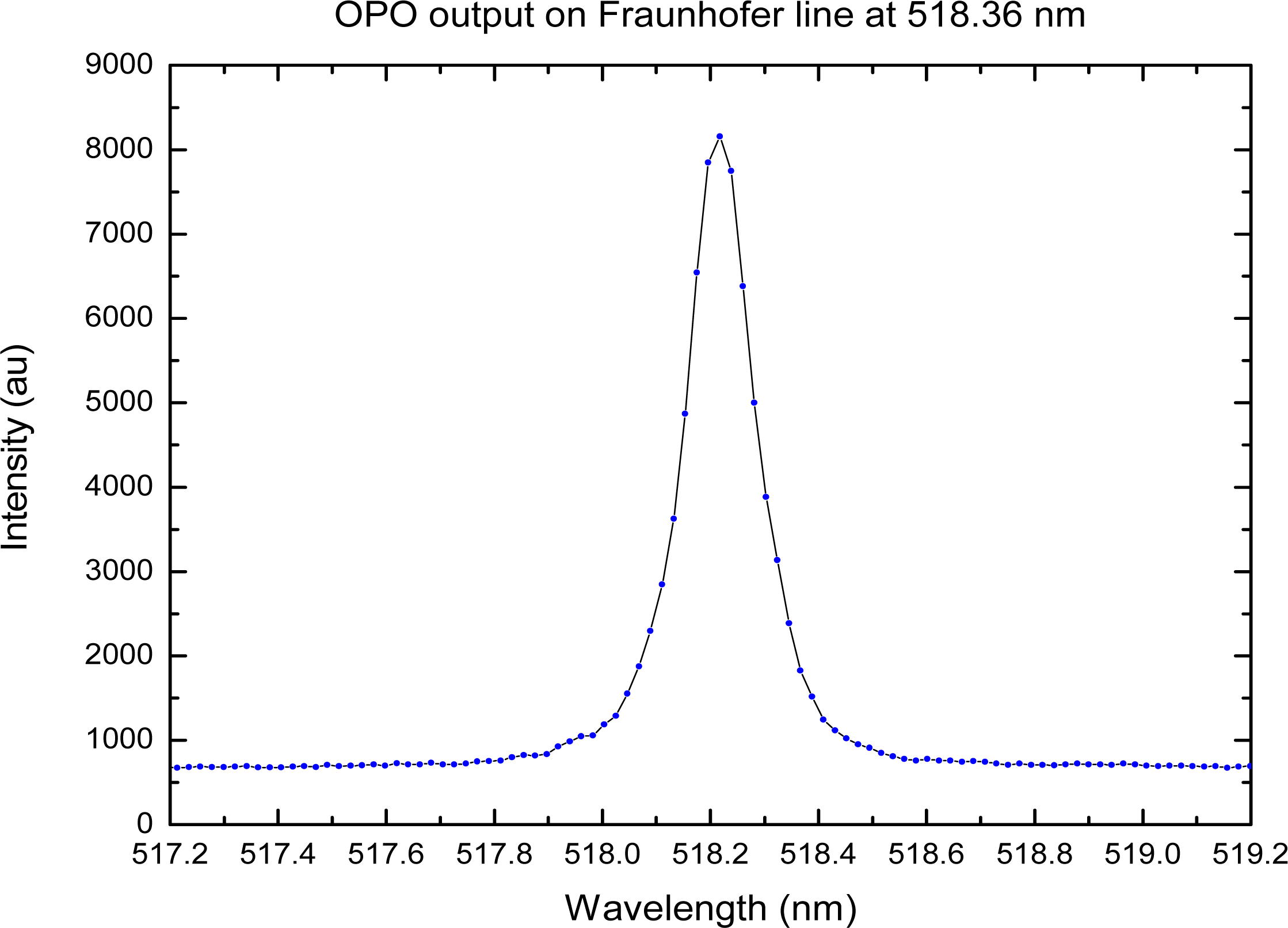
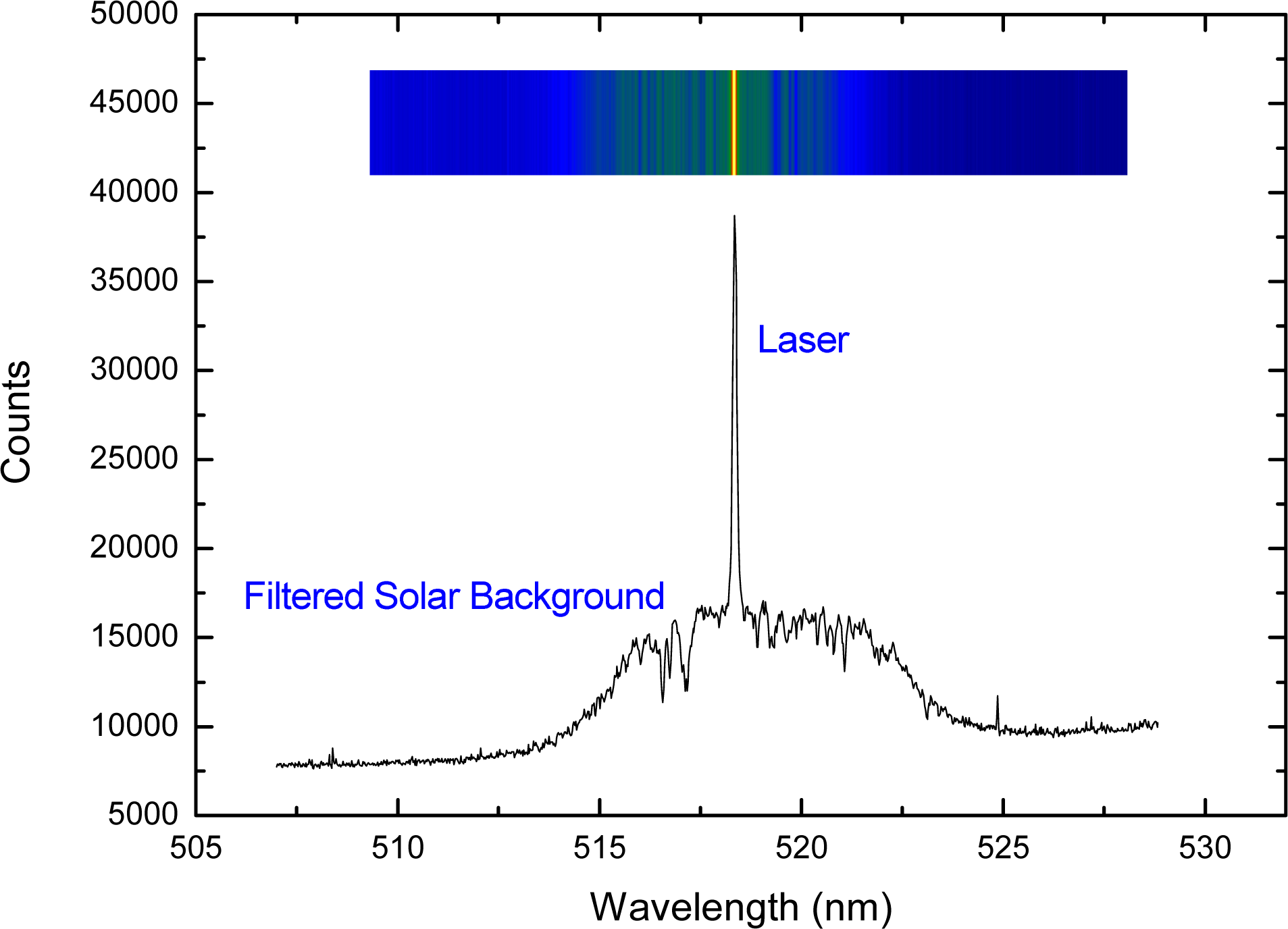
In order to precisely match the laser wavelength and the Fraunhofer lines, the spectral channel using a CCD camera was continuously monitoring the skylight background and the laser backscatters when the laser transmitter was tuning to the minimum of the solar dark line.
Figure 5 shows the superposition of the solar spectrum and the laser signal which fills the absorption dip of Mg Fraunhofer line at 518.2386 nm. The energy of the laser was attenuated for better illustration.
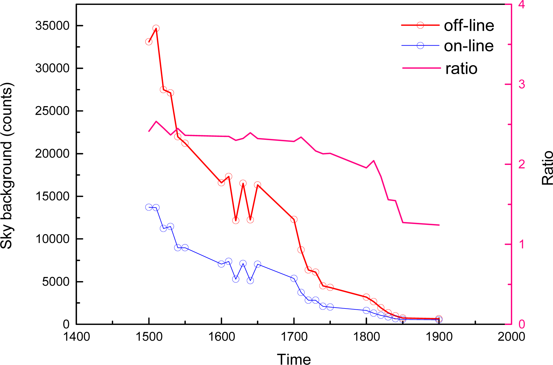
The background level is evaluated for the on- and off-line wavelength of the Fraunhofer line. The decrease of the background from day to night is shown in
Figure 6. The measurements for on- and off-line wavelength were alternately carried out by the one lidar system with the same configurations. It is assumed that all the circumstance factors like sun-zenith angle have the same impact on these very close wavelengths. The maximum of the background was observed at 15:00 pm because of the telescope pointing approximately at the sun. It can be seen that the difference in on- and off-line wavelength for the solar background is of the order of 70%, which is less than the theoretical estimation. This is mostly due to the insufficient resolution of the spectrograph. Solar noises whose wavelength is not in a superposition with laser signal are also important in SNR. As we use a rotating grating system with the blocking ratio of OD (Optical Density) 6 (corresponding to 10
−6). In order to compress the solar background and the stray light in the grating system, an additional band-pass filter having a linewidth of 10 nm and the blocking ratio of OD 5 is used between the telescope and the input port of the receiving fiber. Thus the total blocking ratio is about OD 11 that is sufficient for the solar background compression out of the spectral region of the Fraunhofer line. In normal case, solar background light comes into the photomultiplier through the filter because of the low blocking ratio of the spectrograph. In this case, the narrow band Fraunhofer absorption line is this not so effective in decreasing background solar background signal.
The output laser is tuned to 518.2386 nm (on-line) and 518.65 nm (off-line), respectively. Then we analyses the lidar SNR according to the lidar returned signal. The SNR is defined as
Equation (1):
where N
s is laser backscattering signal, N
b is the noise introduced by photons of the sky background, and N
e is the noise from the dark current and readout electronics. N
b and N
e are estimated by the square of the standard deviation of the lidar return signal from the far distance where the background noise and electronics noise dominate.
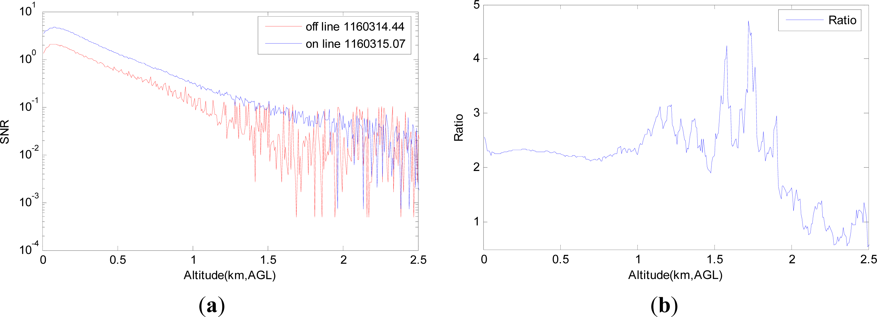
Figure 7a shows the SNR of the returned signal on-line and off-line measurements at 07:00 UTC (15:00 LST). The ratio of on-line SNR to off-line SNR is calculated according to
Equation (2). The SNR on-line is obviously higher than the SNR off-line as shown in
Figure 7b.
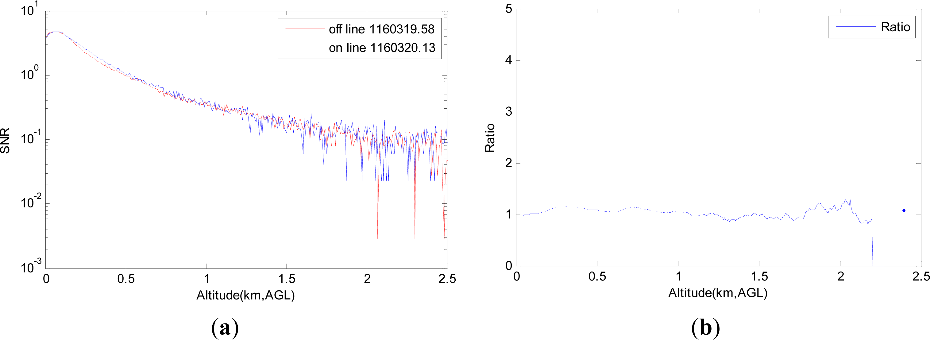
For further contrast,
Figure 8a shows the SNR of the returned signal on-line and off-line measurements at night for the same day while
Figure 8b shows the ratio between them. As
Figure 8 presents, the SNR for the on-line and off-line wavelength are almost equivalent at night measurement. To draw a conclusion, it is very significant to tune the OPO output laser to the minimum of the solar dark line in order to improve the SNR of the Fraunhofer lidar, especially for daytime measurements.
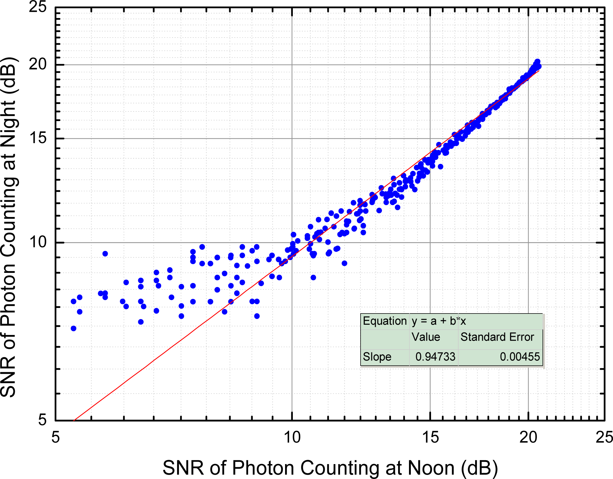
The above lidar return signals were taken at clear and stable weather. In order to eliminate the pulse energy jitter and long term power drift of the transmitting laser, which is prominent for the OPO laser we used, an extra photomultiplier was adopted as reference to eliminate the variation of the laser power. The SNR of the lidar backscatter signals on 3 June 2011 at both noon and night are compared in
Figure 9. The analysis shows that the SNR of the measurements in the daytime are almost equivalent to that of night measurements for SNR > 10 decibels. The variation of the SNR between daytime and nighttime is less than ±1 decibels. For the far distance lidar return, night measurements have better SNR than the daytime n mnmeasurement due to the lower background noise at night (for SNR < 10 decibels).
4. Atmospheric Boundary Layer Observations
According to the above analysis, the prototype lidar exhibits the advantage of photon counting at wavelengths corresponding to Fraunhofer lines in the green spectral region with strong solar irradiance. Two measurement cases obtained at different meteorological and aerosol conditions, are presented to demonstrate the capability of the Fraunhofer lidar prototype for the atmospheric boundary layer (ABL) observation. The lidar was located at the Laoshan campus of the Ocean University of China 6 km away from the seashore and the elevation is 74 m above the mean sea level, where the longitude and latitude is 36.16°N and 120.49°E respectively. As the prototype lidar consists of only an elastic scattering channel, we adopt the well-known Fernald method [
26] to retrieve the aerosol extinction coefficient in the boundary layer. It is requested to determine the reference altitude before calculating the aerosol extinction coefficient of a certain altitude, which is lower than the reference altitude. In this article, the reference altitude is determined at 2–3 km where the aerosol extinction coefficient of the altitude is 0.13 km
−1. To solve the underconstrained lidar equation scince it is associated with two unknowns for one equation, we need to know an extinction-to-backscatter ratio, so-called “lidar ratio”, to retrieve the aerosol extinction coefficient. Lidar ratio is related to the size, the shape, and the composition of the particles. The measurements were held in the summer and the sea breeze is a regular feature of the summer season. The lidar ratio for the marine aerosol is between 20 to 35 sr [
27]. The aerosol optical depths (AOD) can be used to retrieve an average lidar ratio [
28]. For this study, the Moderate Resolution Imaging Spectroradiometer (MODIS) derived AOD was used for the case of boundary layer measurement in cloudless conditions and was used for the lidar ratio inversion.
The evolution of the atmospheric boundary layer under cloudless conditions during daytime is shown first (3 June 2011). In the second case (24 August 2011), the boundary layer with more variation (clouds on top of the boundary layer) is discussed and validated with the results of the space-borne lidar CALIOP onboard CALIPSO satellite.
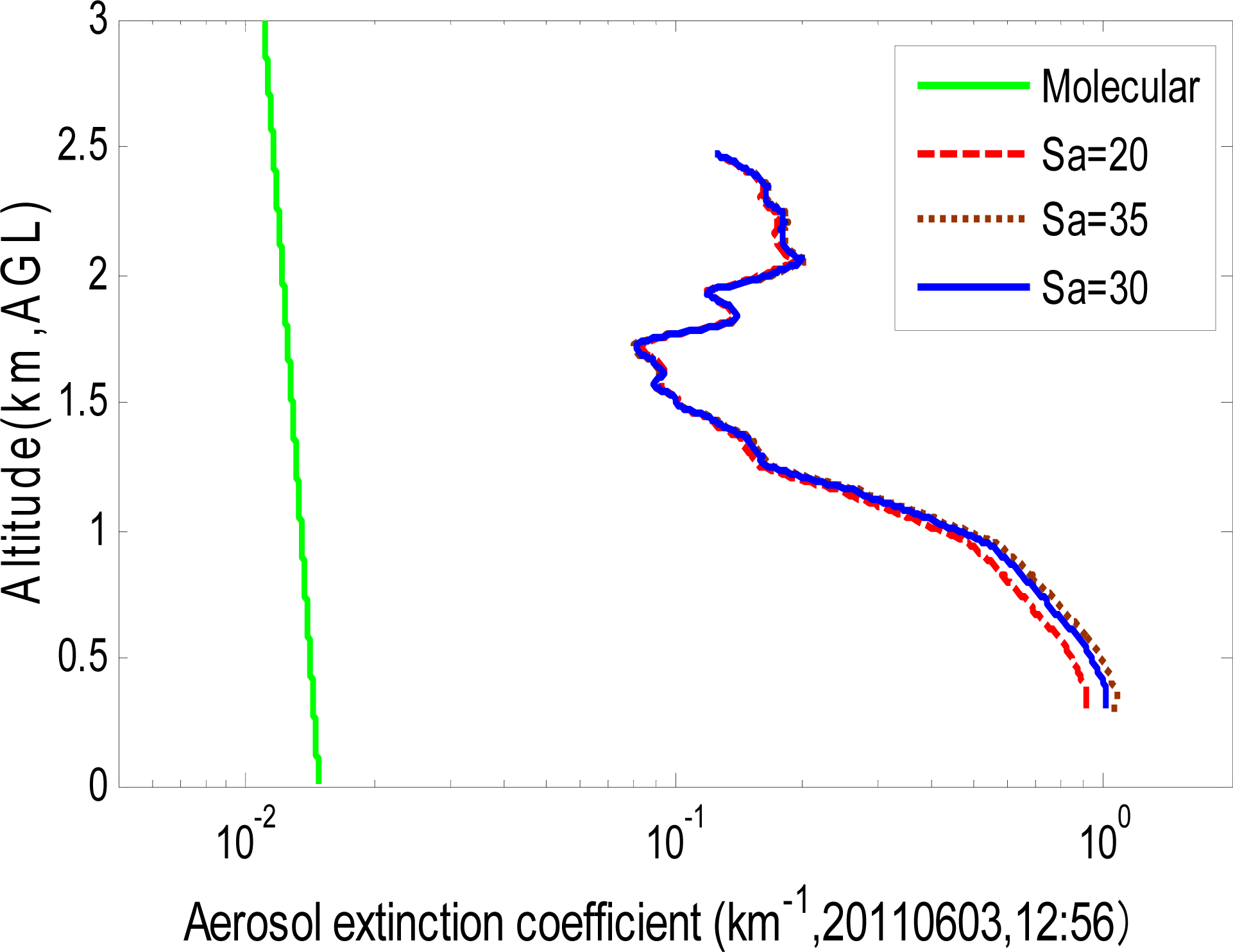
Figure 10 presents the aerosol extinction coefficient profile above the ground level on June 3, 2011, for the lidar ratio of 20, 30 and 35 sr, respectively. As shown in this figure, although it has slight difference when the altitude is lower than 1 km, the tendency of these three profiles is consistent. A ratio of 30 sr is used in this work.
In order to detect the vertical profile of the extinction coefficient and compare the detection performance between daytime and nighttime, the experiments were carried out when it was sunny and cloudless. The measurement was performed from 10:00 am to 20:00 pm when the weather conditions allowed from May to August. The 6 min averaged lidar profiles, comprising 3,600 shots acquired, were used for the extinction coefficient inversion.
For the first case, one scene of the boundary layer during clear sky condition is shown.
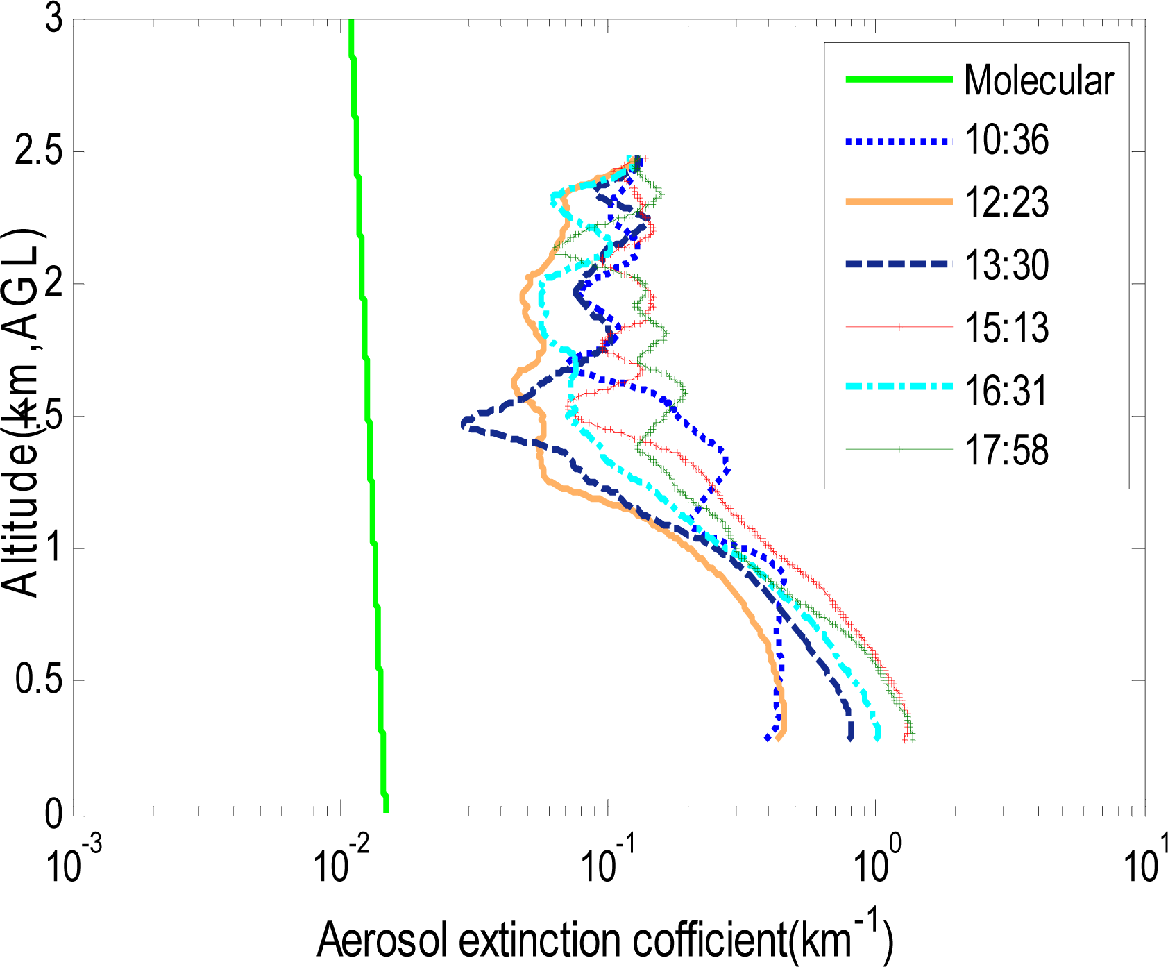
Figure 11 presents the vertical extinction coefficient profiles for different times on 3 June 2011. As shown in the figure, the aerosol under 1.5 km increases slowly from 02:30 to 10:30 UTC (from 10:30 to 18:30 LST) and decreases from 08:31 to 11:31 UTC (from 16:31 to 19:31 LST). Meanwhile, the aerosol above 1.5 km has no obvious variation. According to the meteorological data, the relative humidity is 93%∼96% on 3 June. The aerosol extinction coefficient is large because of the moisture absorption effect of the aerosol particles. The extinction coefficient is retrieved above an altitude of around 400 m because of the loss of overlap between the laser beam and the telescope field of view.
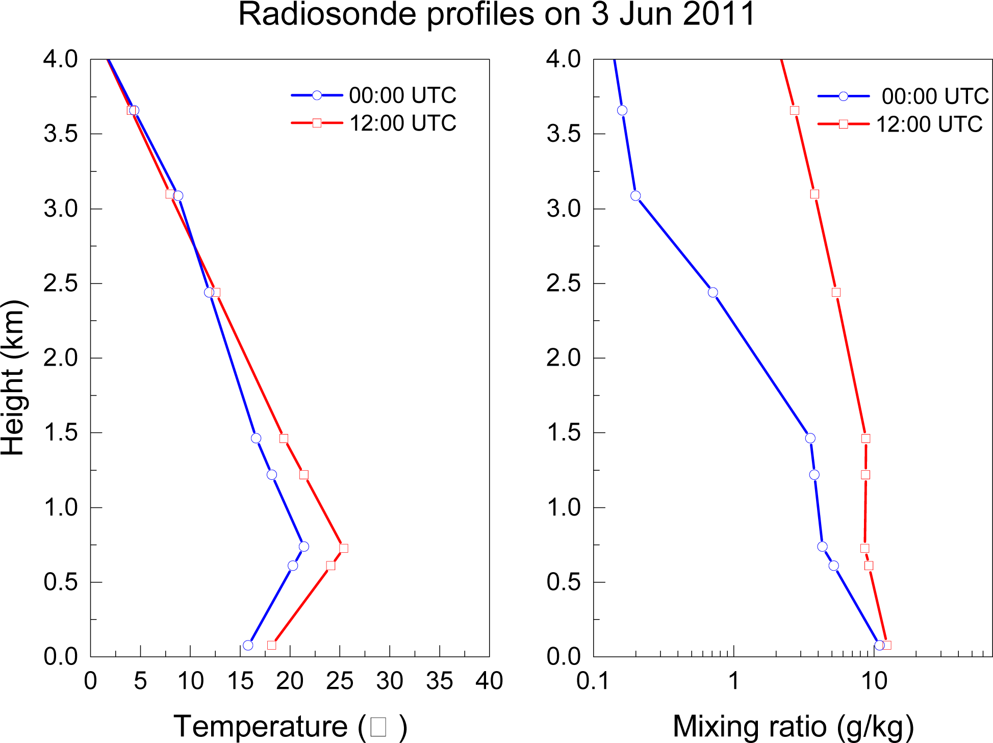
The height of the atmospheric boundary layer can be estimated using the potential temperature profile. This height is identified to be the height at which the potential temperature is subject to a steep increase. The radiosonde profiles on 3 June 2011 are plotted as
Figure 12. The radiosonde was launched at approximately 8:00, 20:00 LST at the Qingdao Meteorological Station, where the longitude and latitude is 36.06°N and 120.33°E respectively. The inversion layer is obviously indicated at around 737 m (00:00 UTC, 08:00 LST) and 725 m (12:00 UTC, 20:00 LST), respectively in the radiosonde profiles. At the inversion layer, the water vapor mixing ratio at the night (12:00 UTC, 20:00 LST) is 8.63 g/kg, much higher than the mixing ratio of 4.28 g/kg in the morning (00:00 UTC, 08:00 LST).
From the Fraunhofer lidar observation, the height of the boundary layer is indicated by a sharp change in the extinction profile. To investigate the development and variation of the aerosol boundary layer,
Figure 13 shows the boundary layer evolution in terms of the extinction coefficient observed with the Fraunhofer lidar on 3 June 2013. The maximum detection height is around 2.48 km based on the SNR threshold. For this study, 30 min averages were used to obtain statistically meaningful boundary layer height. A stable boundary aerosol layer below approximately 1 km is observed. According to the local meteorological report there was a sea breeze (south-west wind) and fog emerging in the afternoon. As shown in the
Figure 13, a lower layer with a height of below 800 m is due to the sea breeze front emerging at 15:00 LST. The boundary layer fluctuates as the front passes underneath it, showing how sea breeze propagation may produce gravity waves in the overlying stable inversion layer.
The other measurement on 24 August 2011 is observed using the Fraunhofer lidar for case study with strong variability.
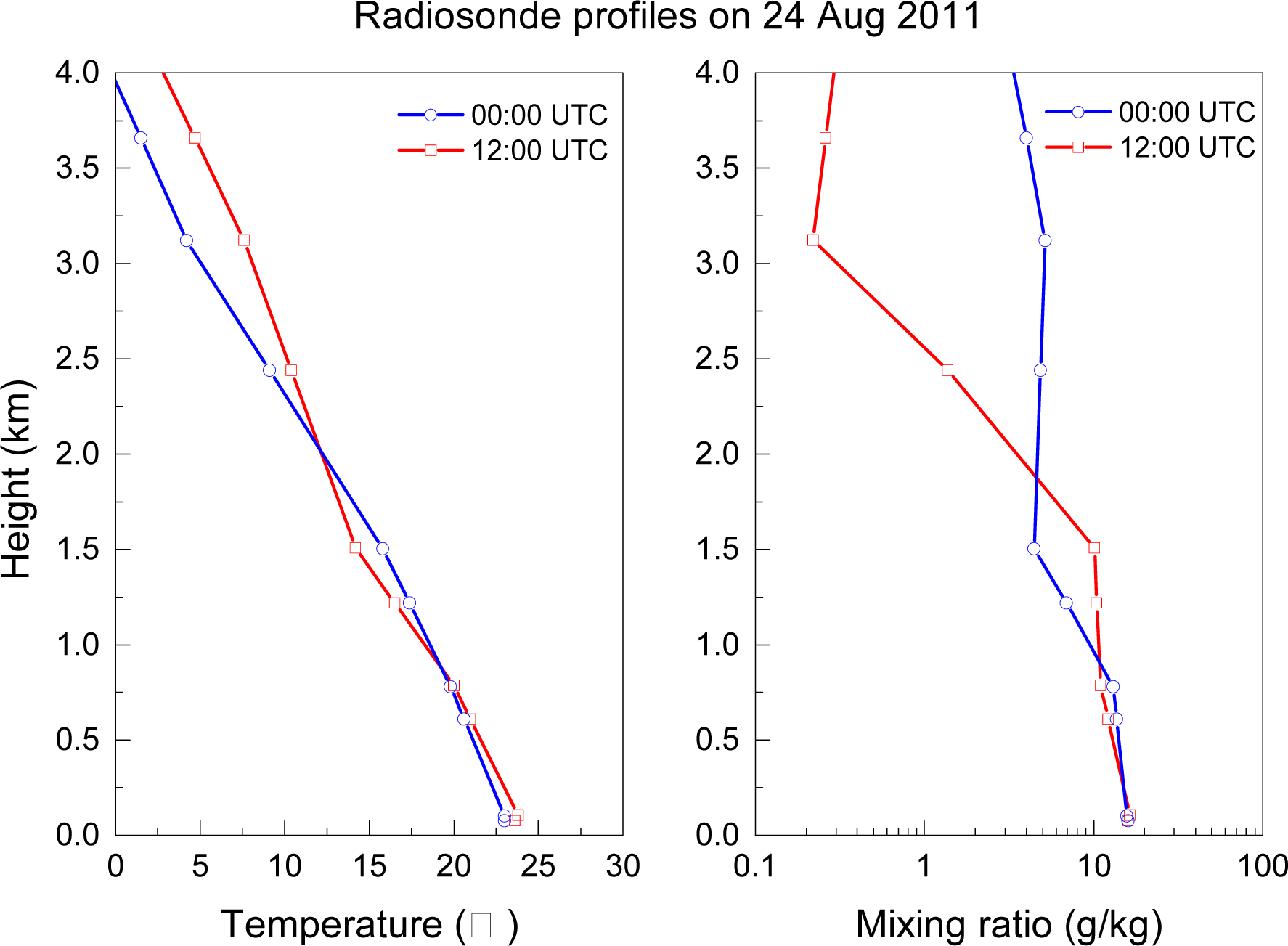
Figure 14 presents the vertical extinction coefficient profile on August 24, 2011. As shown in the figure, the aerosol under 1.5 km varies slowly while obvious variation appears when the altitude is above 1.5 km. Moreover, the variation is almost one order of magnitude bigger because of the existence of low cloud at 03:16 UTC (11:16 LST). The radiosonde profiles are shown in
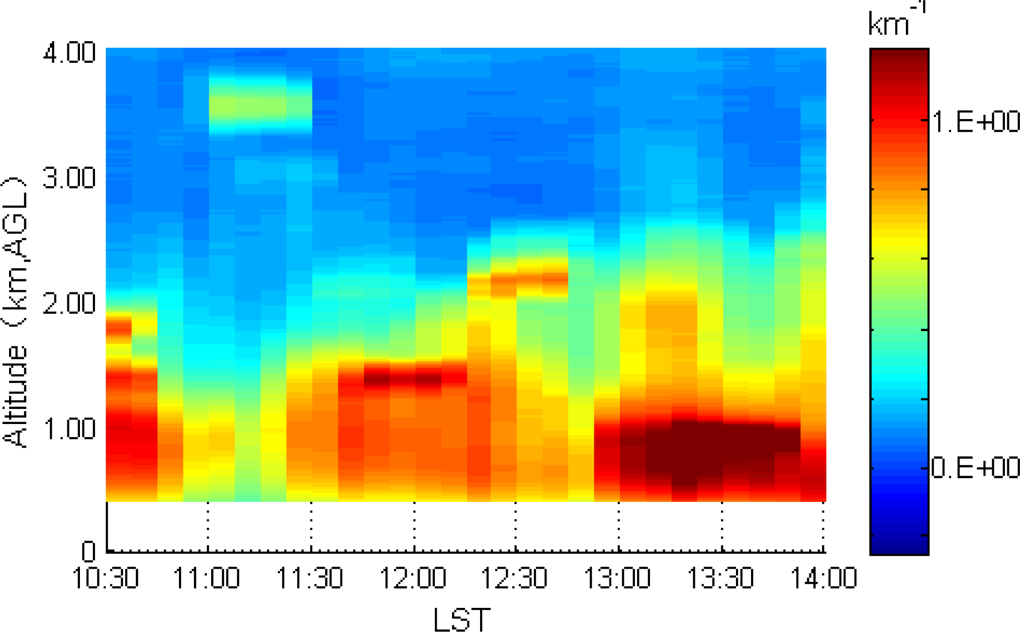
Figure 15. There is not a distinct inversion layer in the temperature profile to be used to estimate the height of the boundary layer. The feature of an abrupt decrease in the water vapor mixing ratio Profile is used to mark the boundary layer around 1.5 km. The time-height-indicator of the extinction coefficient in
Figure 16 indicates that there are two layers of semi-transparent cloud occupation from 2:52 to 3:48 UTC (from 10:52 to 11:48 LST). The lower cloud layer top and bottom altitudes are identified as 3 km and 2.7 km. The higher cloud layer top and bottom altitudes are found as 3.9 km and 3.6 km. The extinction coefficient profile at 11:16 (blue plot in
Figure 15) also shows a high value at the height of 3.5 km. The high extinction and variability is obvious below 1.5 km. The averaging time is adjusted to 15 min in this case due to the rapid variation.
It is important to note that daytime Fraunhofer lidar data is, unlike an ordinary Mie lidar, not noisier than that of night-time due to the absorption of the solar background by certain constituents in the solar atmosphere. From the Time-Height-Indicator figures, the aerosol varies obviously from afternoon to the dusk. Because the lidar site is in the suburb of Qingdao, the major environmental influence comes from the atmospheric turbulence rather than human activities.
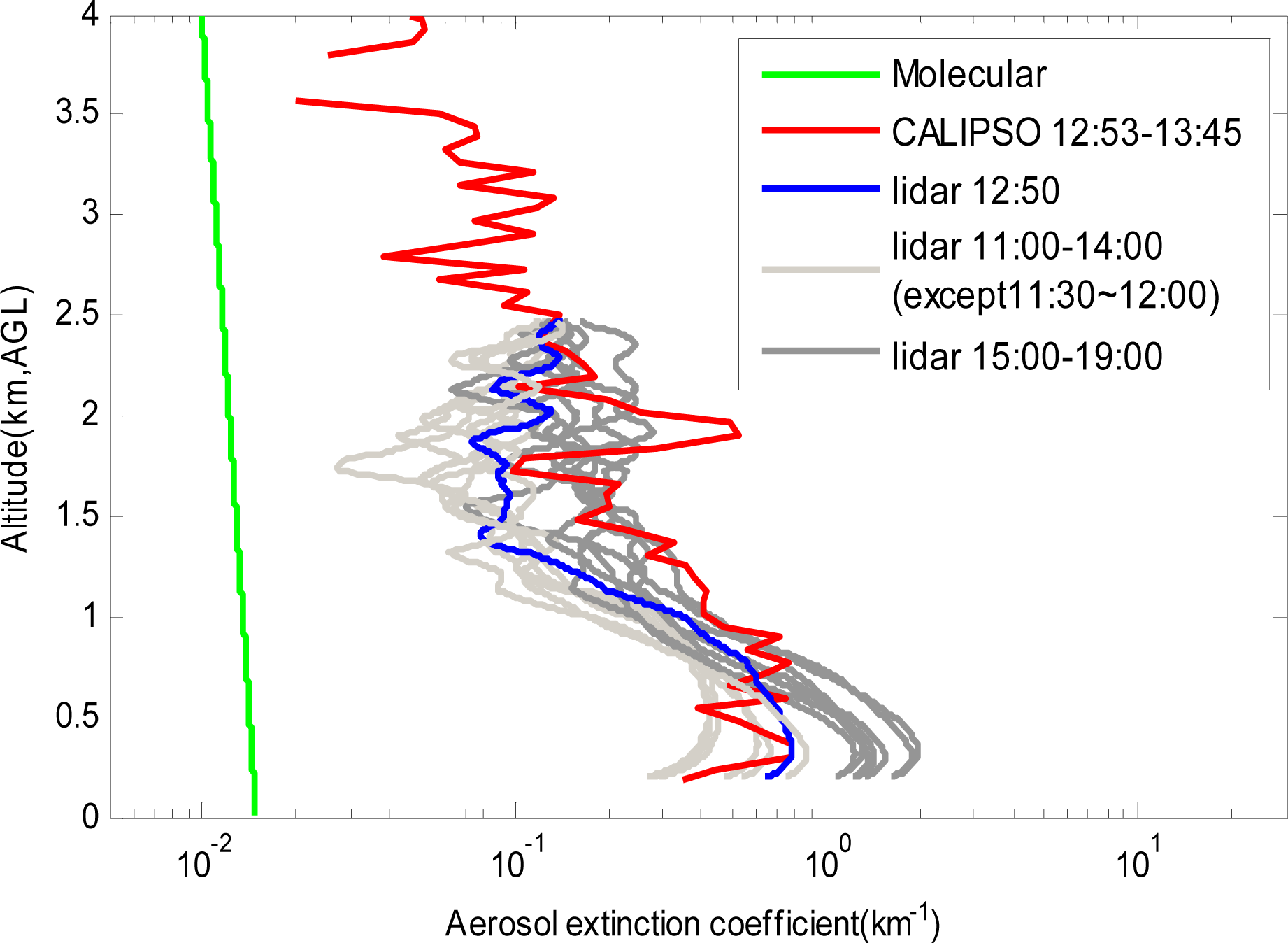
For comparison,
Figure 17 presents the profiles of the aerosol extinction coefficient detected by the Fraunhofer lidar and the CALIOP level-2 aerosol profile product under cloud-free conditions (3 June 2011) with a horizontal resolution of 40 km and vertical resolution of 120 m (backscatter, extinction, and depolarization ratio). CALIOP (Cloud-Aerosol LIdar with Orthogonal Polarization) is a two-wavelength polarization-sensitive lidar onboard the NASA/CNES CALIPSO satellite (Cloud-Aerosol Lidar and Infrared Pathfinder Satellite Observation), to provide high-resolution vertical profiles of aerosols and clouds as well as on their optical properties at two wavelengths (532 nm and 1,064 nm) [
29]. The Fraunhofer lidar performed measurements before and after the CALIPSO northward-flying over the lidar location within a maximum distance of 46 km at 04:53 UTC (12:53 LST). The averaged CALIOP aerosol extinction profiles between 04:53 and 05:45 UTC (between 12:53 and 13:45 LST) are used for comparison. Spatial and temporal variability of aerosol results in the complex validation analysis of the Fraunhofer lidar measurement by direct comparison with the CALIOP. In this case, although CALIOP overpasses the ground based lidar location with a distance of 46 km, the comparison illustrates that both lidars show consistent trend in the upper part of the ABL (0.7∼1.5 km) considering the spatial inhomogeneity of aerosol distributions.
5. Conclusion
The goal of this work is to measure the lidar backscattered signal in the green spectral region where the solar background is intensively attenuated due to the Fraunhofer absorption lines, making daytime photon counting technique possible. This is the first time, to our knowledge, that Fraunhofer lines are used for planetary boundary layer lidar remote sensing. The prototype lidar exhibits the advantage of not having to use complex noise filtering procedures, representing a viable option for an operational lidar designed to measure the atmosphere during daytime and night. The experiment detects the atmospheric parameters and characteristics of the atmospheric boundary layer. The analysis illustrates that the SNR was improved 2–3 times by operating the lidar at the wavelength in solar dark lines. However, the stability of the prototype is to be improved because of technical limitations. The OPO laser was the only accessible laser source at the experimental time, which represents a suitable solution for prototyping, but cannot be used for accurate and effective measurements for PBL. The advantage of using an OPO laser is its tunability to cover selected Fraunhofer lines in one lidar system. But, the OPO laser needs to achieve better frequency stability so that the frequency drift can be inhibited and the detector can accurately match with the receiving bandwidth. But, the disadvantages of using an OPO laser are low efficiency and poor beam quality. The OPO efficiency and other issues in the laser system will probably lower the outgoing laser energy by a factor of 2–3, compared to transmitting the 532 nm wavelength directly. Those efficiency losses of the OPO laser counteract the benefits of the SNR improvement by tuning the laser to the Fraunhofer lines. Therefore, more efficient laser transmitter should be designed for experiments.
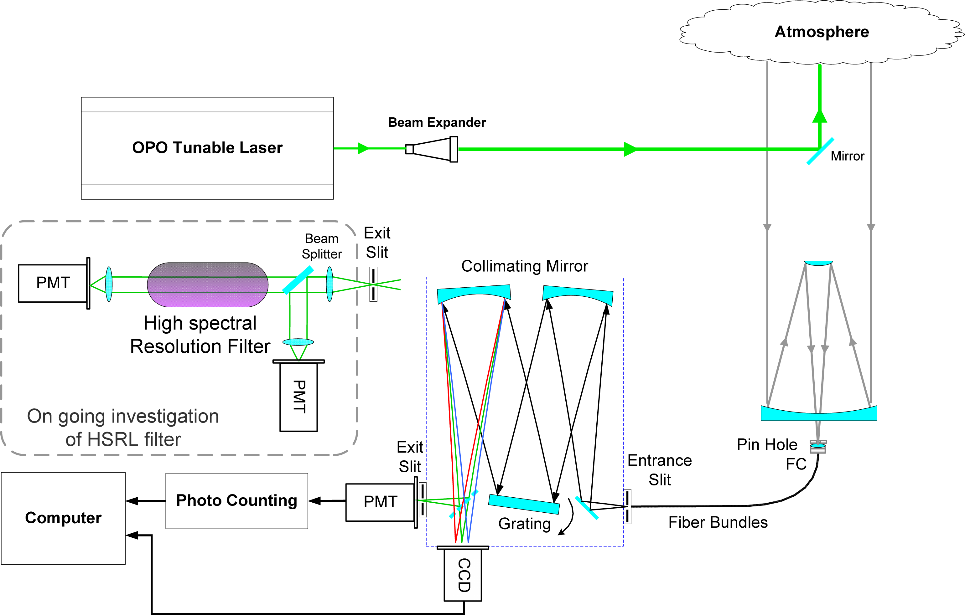
The diagram in the dashed rectangle in
Figure 2 shows the ongoing investigation to assess high spectral resolution filter coincide with wavelengths of candidate notable Fraunhofer lines, such that it is possible to isolate the signal from the solar noise and take advantage of traditional HSRL for wind, temperature and aerosol probing. There are a large number of absorption lines of iodine around solar Fraunhofer line by Magnesium at 516.4521 nm, 517.0414 nm and 518.2386 nm. The idea and primary experiments in this paper present a possible solution to the operational observation problems normally associated with photon counting lidar for green wavelengths, and guarantee further investigations on lidar systems.


