Assimilation of ICON/MIGHTI Wind Profiles into a Coupled Thermosphere/Ionosphere Model Using Ensemble Square Root Filter

Highlights

What are the main findings?

• The implementation of an Ensemble Square Root Filter (EnSRF) to assimilate real ICON/MIGHTI neutral wind profiles into the TIE-GCM significantly enhanced the model’s accuracy, reducing the Root Mean Square Error (RMSE) for both zonal and meridional wind components by approximately 45% to 50% compared to the control run.
• While zonal wind assimilation demonstrated strong model memory and sustained forecast skill, the meridional wind exhibited a “short memory” characteristic where improvements dissipated rapidly within one hour.

What are the implications of the main findings?

• The rapid decay of forecast skill for meridional winds underscores the dominance of rapidly evolving wave structures in thermospheric circulation, emphasizing the critical necessity of employing high-frequency assimilation cycles (e.g., hourly updates) to effectively constrain the instantaneous wind state.
• The assimilation system does not merely reduce numerical errors but actively sharpens the spatial definition of circulation cells and cross-equatorial flows, providing a high-fidelity state estimate that is essential for advancing the understanding of complex interactions within the ionosphere-thermosphere system.

Abstract

Precise characterization of the thermospheric neutral wind is essential for comprehending the dynamic interactions within the ionosphere-thermosphere system, as evidenced by the development of models like HWM and the need for localized data. However, numerical models often suffer from biases due to uncertainties in external forcing and the scarcity of direct wind observations. This study examines the influence of incorporating actual neutral wind profiles from the Michelson Interferometer for Global High-resolution Thermospheric Imaging (MIGHTI) on the Ionospheric Connection Explorer (ICON) satellite into the Thermosphere Ionosphere Electrodynamics General Circulation Model (TIE-GCM) via an ensemble-based data assimilation framework. To address the challenges of assimilating real observational data, a robust background check Quality Control (QC) scheme with dynamic thresholds based on ensemble spread was implemented. The assimilation performance was evaluated by comparing the analysis results against independent, unassimilated observations and a free-running model Control Run. The findings demonstrate a substantial improvement in the precision of the thermospheric wind field. This enhancement is reflected in a 45–50% reduction in Root Mean Square Error (RMSE) for both zonal and meridional components. For zonal winds, the system demonstrated effective bias removal and sustained forecast skill, indicating a strong model memory of the large-scale mean flow. In contrast, while the assimilation exceptionally corrected the meridional circulation by refining the spatial structures and reshaping cross-equatorial flows, the forecast skill for this component dissipated rapidly. This characteristic of “short memory” underscores the highly dynamic nature of thermospheric winds and emphasizes the need for high-frequency assimilation cycles. The system required a spin-up period of approximately 8 h to achieve statistical stability. These findings demonstrate that the assimilation of data from ICON/MIGHTI satellites not only diminishes numerical inaccuracies but also improves the representation of instantaneous thermospheric wind distributions. Providing a high-fidelity dataset is crucial for advancing the modeling and understanding of the complex interactions within the Earth’s ionosphere-thermosphere system.

1. Introduction

The Earth’s thermosphere, extending from approximately 90 km to over 600 km altitude, is a highly dynamic region governed by complex interactions between solar forcing, magnetospheric energy inputs, and upward propagating atmospheric waves. Among the state variables characterizing this region, the thermospheric neutral wind plays a pivotal role [1,2]. It is a primary driver of the ionospheric dynamo, generating electric fields that control plasma drifts and the morphology of the equatorial ionization anomaly (EIA) [3]. In the mid-latitude region, vertical gradients in horizontal winds are the primary mechanism for the formation of Sporadic E (Es) layers via wind shear theory [4]. In the equatorial sector, zonal winds modulate the pre-reversal enhancement (PRE) which triggers Equatorial Plasma Bubbles (EPBs), whereas transequatorial meridional winds can suppress their growth by altering flux tube conductivity [5]. As noted in recent studies, thermospheric winds significantly influence the high-latitude Tongue of Ionization (TOI) by regulating the plasma supply from sub-auroral regions and controlling its morphological evolution from double to single structures [6]. Furthermore, neutral winds significantly influence the transport of momentum and energy, modulating the thermospheric mass density distribution, which is critical for calculating the orbit determination and drag of low-Earth orbit (LEO) satellites [7].

Accurate specification of global thermospheric winds continues to be a challenging endeavor in the field of space physics and aeronomy, despite the significance of this task and the technological advancements in measuring upper atmospheric wind fields. Unlike the lower atmosphere, which has dense networks of sensors, the thermosphere lacks direct wind measurements—often referred to as the “thermospheric wind gap.” While ground-based Fabry–Perot Interferometers (FPIs) provide valuable local profiles [8,9], they are geographically sparse and typically limited to nighttime operations. Satellite missions, such as the Gravity Recovery and Climate Experiment (GRACE) and the Challenging Minisatellite Payload (CHAMP), have primarily provided accelerometer-derived mass densities rather than direct wind vectors. Consequently, theoretical General Circulation Models (GCMs), such as the TIE-GCM or WACCM-X, are often relied upon to estimate wind fields. However, these models are subject to uncertainties in high-latitude forcing and lower-boundary conditions, leading to discrepancies between simulations and reality, particularly during geomagnetic storms.

To bridge the gap between sparse observations and theoretical models, Data Assimilation (DA) techniques have emerged as a powerful tool. DA optimally combines observations with a background model based on their respective error statistics to provide a “best estimate” (analysis) of the atmospheric state. In particular, the Ensemble Kalman Filter (EnKF) has gained prominence due to its ability to handle the flow-dependent background error covariance of the coupled thermosphere-ionosphere system [10].

Early applications of EnKF in the upper atmosphere focused on assimilating electron density or neutral mass density to infer unobserved wind states through multivariate cross-correlations [11,12,13]. While effective, these indirect methods rely heavily on the accuracy of the model’s physics to couple mass and momentum fields. NASA’s Ionospheric Connection Explorer (ICON) mission, equipped with the Michelson Interferometer for Global High-resolution Thermospheric Imaging (MIGHTI), has enabled a transformative step in understanding the ionosphere. This mission aims to explore the boundary between Earth and space, examining the physical connection between our world and the space environment, particularly focusing on the ionosphere’s variability influenced by solar and atmospheric factors. MIGHTI provides unprecedented daytime and nighttime wind vectors at low and mid-latitudes [14]. Recent studies, such as Hsu et al. (2021) [15], have utilized observing system simulation experiments (OSSE) to show that incorporating these simulated wind observations can substantially decrease inaccuracies in ionospheric electrodynamics models. Furthermore, applying advanced deterministic filtering algorithms to real ICON/MIGHTI data remains relatively unexplored in the context of assimilation systems.

To address these challenges, we developed a thermospheric data assimilation system based on the Ensemble Square Root Filter (EnSRF) [16]. By assimilating real wind profiles from the ICON/MIGHTI instrument into the TIE-GCM, we aim to significantly enhance the model’s accuracy. To our knowledge, this is one of the initial efforts to specifically apply the EnSRF algorithm for the assimilation of real space-based thermospheric wind measurements. By conducting assimilation experiments with actual satellite data, we aim to: (1) evaluate the performance of EnSRF in the sparse data environment of the thermosphere; and (2) quantify the enhancement in global wind field specification has been driven by the direct assimilation of observations from the MIGHTI instrument.

2. Data and Methodologies

2.1. Data

• ICON/MIGHTI

The Ionospheric Connection Explorer (ICON) mission was launched in 2019 with the primary objective of understanding the coupling between the ionosphere and thermosphere [14]. The spacecraft operates in a low Earth orbit with a 27° inclination at an altitude of approximately 575 km, completing an orbital period every 97 min. Among its four instruments, the Michelson Interferometer for Global High-resolution Thermospheric Imaging (MIGHTI) is designed to determine horizontal neutral wind vectors and temperatures within the 90–300 km altitude range [17]. MIGHTI employs the Doppler Asymmetric Spatial Heterodyne (DASH) technique to achieve these measurements. By monitoring the atomic oxygen airglow emissions—specifically the green line (O(1S) at 557.7 nm) and the red line (O(1D) at 630.0 nm)—the instrument detects minute wavelength variations caused by the motion of the neutral atmosphere [18]. These Doppler shifts are measured as phase shifts in the interferometric fringe patterns, which are then inverted to retrieve line-of-sight wind velocities. To meet its scientific goals, MIGHTI adheres to stringent precision requirements: a wind speed accuracy of 8.7 m/s is required for altitudes below 105 km and above 200 km, while a precision of 10 m/s is maintained for the intermediate region between 105 km and 200 km [14].

Figure 1 shows the wind field distribution map based on ICON’s 1 h time window observation data. This study utilizes MIGHTI Level 2.2 v05 data, which includes the neutral wind component along the latitudinal circle and the meridional wind component perpendicular to the latitudinal circle.

Figure 1. ICON Satellite 1 h Coverage (21 December 2019, 6UT to 21 December 2019, 7UT); (a) shows the location of the observation; (b) displays zonal wind distribution; (c) displays meridional wind distribution.

Makela et al. (2021) conducted an extensive satellite-ground coordination campaign using a global network of observatories [19]. The validation strategy was stratified by altitude, employing Fabry–Perot Interferometers (FPIs) to validate the F-region Red Line measurements (~250 km) and Meteor Radars to validate the E-region Green Line measurements (~90–100 km). In the middle and upper thermosphere, comparisons with coincident observations from FPI stations across North America, South America, and Northern Africa demonstrated a high degree of consistency. Statistical analyses revealed that correlation coefficients for nighttime zonal and meridional winds typically ranged between 0.7 and 0.9. Crucially, despite the inherent geometric disparity between the satellite’s limb-integrated view and the ground-based localized measurements, the mean systematic bias remained within ±10 m/s. These results strongly support the effectiveness of the MIGHTI algorithm in eliminating zero-point drift, as evidenced by the successful application of software-based methods in various contexts [18,19]. Unlike previous versions, MIGHTI v05 wind products utilize an absolute zero-wind reference based on instrument calibration rather than the HWM model, making them an independent and objective standard for validating data assimilation results [3,18].

In the lower thermosphere (~90–100 km), the validation against Meteor Radars focused on the instrument’s capability to capture large-scale dynamic structures. The analysis indicated that MIGHTI accurately reproduces dominant tidal signatures—specifically semidiurnal and diurnal tides—with highly consistent phase and amplitude structures relative to the radar data. While instantaneous deviations were observed, resulting in a measurable Root Mean Square Error (RMSE), these discrepancies were attributed to active small-scale gravity waves and significant differences in sampling volumes (line-of-sight integration versus volumetric scattering). However, these differences remained statistically within the expected bounds of geophysical variability and measurement uncertainty boundaries [18].

The ground-based validation confirms that MIGHTI provides high-precision wind data across its vertical profile. From the mean state of F-region background winds to the tidal wave structures in the E-region, MIGHTI observations maintain high consistency with independent ground standards, exhibiting minimal systematic error and establishing the dataset as a reliable benchmark for global thermospheric dynamics research.

• TIE-GCM

The Thermosphere Ionosphere Electrodynamics General Circulation Model (TIE-GCM) is one of the most widely used first-principles models, developed at the National Center for Atmospheric Research (NCAR). TIE-GCM self-consistently solves the coupled momentum, energy, continuity, and electrodynamic equations for the thermosphere–ionosphere system, driven by solar and geomagnetic inputs [20]. This study employs the TIE-GCM version 2.0 model, featuring a resolution of 2.5° in both latitudinal and longitudinal directions. It comprises 144 meridional and 72 zonal grid points, with 57 model layers in the vertical direction spaced at quarter-level intervals. The total number of grid points in the background field is 590,976. The spatial resolution has improved by a factor of eight compared to the previous version with a 5° resolution, owing to the refinement of the grid in latitude, longitude, and vertical scale height [13]. The TIE-GCM was driven by observed F10.7 index to capture the realistic variations in solar EUV radiation, which governs the heating and ionization of the thermosphere. To establish a controlled background for data assimilation, geomagnetic forcing was kept constant with the Kp index fixed at 2.0. Under these quiet conditions, the high-latitude electric potential and auroral patterns were specified by the Heelis model [21]. This setup isolates the impact of solar cycle variations on the background state while excluding complex magnetospheric storm dynamics.

The lower boundary of the TIE-GCM (about 97 km) serves as the interface for upward-propagating atmospheric waves (tides and planetary waves) originating from the mesosphere and lower atmosphere. Proper specification of this boundary is critical for capturing the “meteorological” variability of the ionosphere-thermosphere system. Standard TIE-GCM simulations typically rely on the Global Scale Wave Model (GSWM) [22] which prescribes climatological migrating tides. However, GSWM assumes a steady-state atmosphere and fails to capture day-to-day weather variability or non-migrating tides. Conversely, while direct satellite observations (e.g., TIMED/SABER and TIDI [23,24]) capture real events, they suffer from asynoptic sampling limitations [25], making it difficult to construct a continuous global boundary without aliasing. To mitigate these limitations and reduce systematic model errors, this study utilizes the Hough Mode Extension (HME) method driven by the observations from the ICON [22,26].

Specifically, the lower boundary is forced by tidal modes derived from neutral wind and temperature measurements obtained by MIGHTI. The HME technique decomposes these high-precision observations into spectral basis functions (Hough modes), constructing a mathematically continuous and globally consistent boundary field.

Although the TIE-GCM lower boundary is located at ~97 km, the ICON/MIGHTI observations extending down to ~90 km are integral to the HME process. These observations are used to constrain the decomposition of the neutral atmosphere into a spectrum of tidal Hough modes. These derived modes are then used to analytically reconstruct the global variations in zonal wind, meridional wind, and temperature at the 97 km interface. This approach allows the model to benefit from the extended vertical coverage of the satellite observations, ensuring a robust specification of tidal forcing at the model boundary.

2.2. Methodologies

2.2.1. The Ensemble Square Root Filter

The Ensemble Kalman Filter (EnKF) is a sequential data assimilation method that has been widely applied in atmospheric and oceanic sciences. The EnKF is particularly well suited for assimilating wind observations because it allows nonlinear forecast models such as TIE-GCM to be used without linearization, while estimating flow-dependent background error covariances through an ensemble of forecasts [27]. In each assimilation cycle, the EnKF utilizes a finite number of ensemble members to estimate the state covariance matrix [28]. Standard EnKF approaches require perturbing observations to maintain consistent error statistics, which introduces additional sampling noise. To eliminate this specific source of error, we employ the deterministic Ensemble Square Root Filter (EnSRF) [16]. It is important to clarify that while the EnSRF avoids the sampling error associated with perturbed observations, it does not mitigate the sampling errors inherent in the background error covariance matrix derived from a finite ensemble size. Therefore, maintaining a sufficient number of ensemble members remains necessary to prevent spurious correlations. Unlike the stochastic EnKF, which requires perturbing observations to maintain correct analysis error statistics, the EnSRF updates the ensemble mean and perturbations separately. This approach avoids sampling errors introduced by synthetic observation noise.

Let $X_b$ denotes the N-member ensemble of background state vectors. The ensemble is decomposed into its mean $\overline{X_b}$ and perturbations $X_b^{\prime }$, like $X_{b,i}=\overline{X_b}+X_b^{\prime }$ for the ith member. The ensemble mean is updated using the standard Kalman Filter update equation:

$$\overline{X_{a }}=\overline{X_b}+K\left(Y-H\overline{X_b}\right)$$

(1)

where $\overline{X_a}$ is the analysis mean, $Y$ is the observation, and $H$ is the linear observation operator. The Kalman Gain $K$ is computed using the background error covariance $P^b$ derived from the ensemble perturbations:

$$\begin{gathered} P^b={\displaystyle \frac{X_b^{\prime }{X}_b^{\prime T}}{N-1}} \\ K={\displaystyle \frac{P^b{H}^T}{H{P}^b{H}^T+R}} \end{gathered}$$

(2)

where R represents the observation error covariance.

The distinctive feature of the EnSRF lies in the perturbation update. The analysis perturbations $X_a^{\prime }$ are obtained by applying a linear transform matrix $T$ to the background perturbations:

$$X_a^{\prime }=X_b^{\prime }T$$

(3)

Here, $T$ is constructed to contract the ensemble spread consistent with the reduction in error variance due to the assimilation of data. For a serial processing implementation (processing uncorrelated observations sequentially), $T$ is calculated as:

$$T=I-{\displaystyle \frac{\gamma }{1+\sqrt{1+\gamma }}}·{\displaystyle \frac{{\left(H{X}_b^{\prime }\right)}^T\left(H{X}_b^{\prime }\right)}{N-1}}$$

(4)

where $I$ is the identity matrix, and $\gamma$ represents a scalar factor related to the ratio of the background ensemble variance (in observation space) to the observation error variance. This deterministic transformation ensures that the analysis covariance $P^a$ satisfies the theoretical requirement $P^a=(I-KH)P^b$ without the need for perturbed observations.

2.2.2. Covariance Localization

In the Ensemble Kalman Filtering approach, ensemble samples are utilized to estimate the error covariance between the simulated results and the background state, facilitating optimal estimation. field grid points, thereby calculating the gain K to update background values within a specified range around observation points. To suppress distant spurious correlations arising from finite ensembles and enhance numerical stability, this paper implements localization of the ensemble background error covariance matrix [29].

It is generally accepted that the spatial correlation of the thermosphere meets a Gaussian distribution. Here, the ionospheric correlation is simply decomposed as the product of anisotropies in the meridional, latitudinal, and altitudinal directions. The correlation scales of the thermosphere vary with latitude, altitude, local time, season, and solar activity. According to research by Le Xinan et al., the correlation distance in the latitude direction is set to 10, while the correlation distance in the longitude direction varies linearly from ~40 at mid-latitudes to ~20 at the equator. The correlation distance in the vertical direction increases linearly with altitude: 50 km at 160 km, with an additional 40 km for every 100 km increase in altitude. Therefore, in subsequent assimilation, we use the localized covariance matrix. $B_1$ denotes the covariance between the state space and observation space after correction by the localization weight parameter ${\rho }_1$. $B_2$ denotes the observation spatial error covariance matrix after correction by the localized weighting parameter ${\rho }_2$.

$$\begin{gathered} B_1={\rho }_1·\left(X_b^{\prime }S\right) \\ {B}_2={\rho }_2·\left(S{S}^T\right) \end{gathered}$$

(5)

where $S=H{X}_b-H\overline{X_b}$ and $X_b^{\prime }=X_b-\overline{X_b}$. Therefore, the Kalman gain is adjusted to Equation (6):

$$K={\displaystyle \frac{B1}{B2+(N-1)R}}={\displaystyle \frac{{\rho }_1·\left(X_b^{\prime }S\right)}{{\rho }_2·\left(S{S}^T\right)+\left(N-1\right)R}}$$

(6)

2.2.3. Preprocessing Methods for Observational Data

To ensure the robustness of the assimilation system and to filter out potential gross errors from the raw measurements, a rigorous pre-processing and Quality Control (QC) pipeline was applied to the ICON/MIGHTI neutral wind observations prior to assimilation into the TIE-GCM. The procedure consists of three main stages: gross error removal, vertical regularization, and a background check based on the 3$\sigma$ rule. First, the official data quality flags provided with the MIGHTI Level 2.2 v05 products were checked. Data points indicating potential contamination or instrument errors (Quality < 1) were excluded.

The raw observational profiles often contain high-frequency noise and possess a vertical resolution that differs from the model grid. To mitigate the representativeness error arising from this scale mismatch, the following steps were executed:

Before interpolation, a preliminary screening was performed on the raw profiles. Data points with physically unrealistic values (e.g., wind speeds > 300 m/s during quiet conditions) were rejected.

To align the high-resolution observations with the TIE-GCM’s effective resolution, a two-step vertical processing scheme was employed. First, the cleaned wind profiles were linearly interpolated onto a uniform geometric height grid with a 2 km resolution. Subsequently, a moving average filter with a window size of 5 points was applied to this interpolated grid. This window corresponds to a fixed vertical extent of 10 km, which serves to effectively filter out sub-grid variability—such as small-scale gravity wave perturbations—prior to mapping the data onto the model’s pressure levels. Figure 2 illustrates this process, showing the smoothed profile (orange) effectively capturing the mean structure of the noisy raw observation, a result that is consistent with the principles of mean filtering as detailed in digital image processing literature (blue).

Figure 2. Example of the processed wind profile. (a) Example of the processed zonal wind profile; (b) Example of the processed meridional wind profile. The blue lines represent the raw wind field distribution, while the orange line indicates the wind profile after interpolation and smoothing.

Considering the noise suppression effect brought by the smoothing process, the observational error standard deviation, ${\sigma }_o$ was set to 10 m/s. Finally, a background quality control check was implemented to identify statistical outliers relative to the model state. An observation $y_o$ was rejected if its deviation from the model background counterpart $H\left(x_b\right)$ exceeded three times the total expected error standard deviation:

$$\left|y_o-H\left(x_b\right)\right|\le 3\sqrt{{\sigma }_b^2+{\sigma }_o^2}$$

(7)

$${\sigma }_b=\sqrt{{\displaystyle \frac{1}{N-1}}{\sum }_{i=1}^N{(x_b^i-\overline{x_b})}^2}$$

(8)

where ${\sigma }_b$ is the background error variance derived from the ensemble spread. This ensures that observations inconsistent with the prior ensemble distribution are excluded from the analysis.

After these Quality Control procedures, the number of valid observation points is approximately 5000 for each assimilation window (spanning approximately 100 profiles).

2.3. Experimental Design

In this study, we select 20 ensemble members to generate the initial field. The ensemble members are perturbed by the $F_{10.7}$ to represent the disturbance field, because the TIE-GCM model is driven by solar radiation which is represented by $F_{10.7}$. The initial perturbed $F_{10.7}$ is specified as the real measurement plus a 20 percent random deviation. With the perturbed $F_{10.7}$, TIE-GCM runs from 00:00 UT to 06:00 UT on 21 December to obtain the ensemble initial field. After that time, two kinds of running are designed, i.e., Control Run, and Forecast Run. Control Run is carried out with the ensemble initial field at 06:00 UT on 21 December as the input, running TIE-GCM and obtaining the ensemble output field at 07:00 UT on 21 December. Repeat Control Run until 06:00 UT on 22 December, then we can obtain 24 h Control Run output fields. Note that the Control Run represents the model’s free-running state and contains inherent model biases, rather than representing the absolute ground truth.

Forecast Run takes the initial ensemble field at 06:00 UT on 21 December as the input, running TIE-GCM and obtaining the ensemble output fields at 07:00 UT on 21 December. The output ensemble fields are the background fields. The data assimilation is then conducted at 07:00 UT on 21 December.

The assimilation window is set by 1 h and assimilation is carried out each hour. The observations are used within a half-hour window before and after the analysis time, specifically within 06:30–07:30 UT. The state vector is defined as the zonal and meridional wind. Following the integration of data, the analysis field at 07:00 UT on 21 December was derived, reflecting the concurrent stock market conditions. Using the analysis field, the background field for the next hour can be generated through Forecast Run. Then repeat data assimilation and Forecast Run cycle till 07:00 UT on 22 December, then we can obtain 24 h background fields and analysis fields. During Control Run and Forecast Run, $F_{10.7}$ is set the same as the observations. Figure 3 shows the assimilation cycle.

Figure 3. Schematic of the assimilation cycle. The ensemble system, consisting of 20 members, evolves using the TIE-GCM model. The assimilation process incorporates ICON/MIGHTI observations (Y) hourly from 07:00 UT on 21 December 2019, to 06:00 UT on 22 December 2019. Here, $X_b$ denotes the Background field predicted by the model, and $X_a$ represents the Analysis field updated via the Ensemble Kalman Filter (EnKF).

The Control Run output is compared with the Background field to demonstrate the effects of data assimilation using MIGHTI wind data. In this study, half of the observation data, randomly selected from the total dataset, was utilized for data assimilation, while the remaining data was employed for result validation.

3. Results

3.1. Increment of MIGHTI Wind Data Assimilation

Figure 4 illustrates the hourly evolution of the zonal wind assimilation increments (defined as the analysis field minus the background field, $x_a-x_b$) over a complete 24 h cycle. The increments represent the corrections applied to the TIEGCM background state by the assimilation of ICON/MIGHTI neutral wind observations.

Figure 4. Hourly evolution of the zonal wind assimilation increments (analysis field minus the background field, $x_a-x_b$) over a 24 h period. The subplots display the global distribution of increments from 07:00 UT to 06:00 UT. The black solid lines indicate the ICON/MIGHTI observation tracks. The color scale represents the wind speed correction in m/s, at an altitude of approximately 250 km.

The spatial distribution of the increments is strictly confined to the vicinity of the ICON satellite ground tracks, indicated by the black lines. This localization demonstrates the effectiveness of the covariance localization radius employed in the EnSRF algorithm. By limiting the spatial extent of the updates, the system effectively mitigates the impact of spurious long-range correlations, ensuring that observational information is only projected onto physically relevant grid points surrounding the measurement location. Regions far from the satellite track exhibit near-zero increments (shown in white), confirming that the unobserved background state remains undisturbed where no data is available.

A distinct alternating pattern of positive (blue) and negative (red) increments is observed along the satellite tracks throughout the 24 h period. These wave-like structures suggest that the data assimilation system is primarily correcting large-scale spatial discrepancies consistent with dominant wave modes, such as atmospheric tides. The alternating polarity implies that the background model (TIE-GCM) likely exhibits spatial misalignments in the positioning of wave crests and troughs compared to the observations. The assimilation system successfully captures these coherent deviations and adjusts the wind field distribution accordingly.

The magnitude of the wind increments primarily ranges between ±20 m/s and ±80 m/s, with peak values rarely exceeding ±100 m/s. These corrections are physically consistent with the typical variability of thermospheric winds. The absence of excessively large or noisy increments indicates that the observational error covariance ($R$) and background error covariance (P) are well-balanced, preventing “filter divergence” or shock to the model state.

3.2. Global Winds After 24 h Data Assimilation Cycle

Following 24 h of uninterrupted data assimilation, we derived the comprehensive global wind field distribution. Figure 5 illustrates a comparative analysis of the global zonal wind fields at the 24th hour of the assimilation window, showcasing the effectiveness of advanced data processing and visualization techniques. The panels illustrate three distinct model states: the Background (pre-assimilation, left), the Analysis (post-assimilation, middle), and the Control Run (free-running, right). The altitudes from bottom to top are 150 km, 200 km, 250 km, and 300 km, respectively.

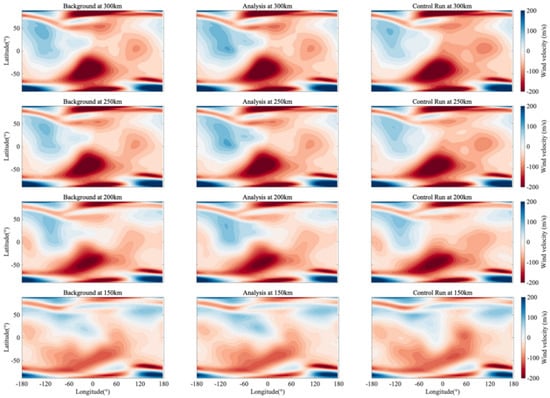
Figure 5. Zonal wind field distribution after 24 h of continuous assimilation. The altitudes, from bottom to top, are 150 km, 200 km, 250 km, and 300 km, respectively. The first column represents the Background field, the second column represents the Analysis field, and the third column represents the Control Run field.

In the southern hemisphere mid-latitudes (approx. 30°S–60°S), the assimilation significantly modulates the intensity of the westward jet. The Control Run exhibits a relatively diffuse jet structure. In contrast, the Analysis field reveals a more concentrated and intensified jet core, particularly visible at 200 km and 250 km altitudes.

The mechanism behind this enhancement is further elucidated by the zonal wind increments shown in Figure 6. The increments are not randomly distributed but exhibit organized, large-scale spatial patterns. For instance, a distinct concentric positive increment (blue) is observed near 60°W (−60° longitude), surrounded by negative adjustments. This coherent structure indicates that the assimilation system is applying targeted structural corrections to specific wind features. This suggests that the TIE-GCM, in its free-running state, tends to underestimate the peak velocity of the thermospheric jet or produce overly smooth features. The assimilation of ICON/MIGHTI data recovers the sharper gradients and stronger wind speeds observed in the actual atmosphere by injecting these spatially coherent increments. It is important to note, however, that the observed ‘sharpening’ of these structures reflects both the physical corrections to the TIE-GCM’s underestimated gradients and the mathematical influence of the localization scheme employed in the assimilation process. While the localization helps in constraining the impact of observations to a physically meaningful range, it may also contribute to the emergence of localized steep gradients. Consequently, the refined structures are likely a combined result of the system rectifying model smoothness and the spatial filtering characteristics of the localization function.

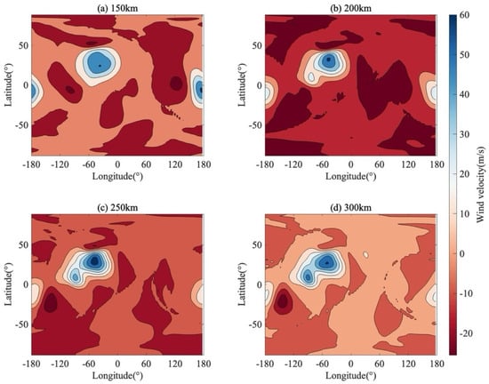
Figure 6. The increment of zonal wind field distribution. The increments are displayed at four distinct altitudinal slices: (a) 150 km, (b) 200 km, (c) 250 km, and (d) 300 km.

Furthermore, the assimilation leads to a noticeable adjustment of the wind speed extrema in the equatorial and northern low-latitude regions. For instance, at 300 km altitude, the zonal wind patterns in the Analysis field exhibit sharper transitions compared to the Control Run. This ‘sharpening’ effect indicates the system’s capacity to introduce finer-scale variability into the wind field, which is often excessively smoothed in the free-running TIE-GCM. By capturing these localized structural deviations (as evidenced by the concentrated increments), the system generates structures and local wind extrema that are spatially consistent with the observations. These adjustments suggest that the assimilation system modifies the model’s representation of zonal flow intensity and spatial variability. The potential mechanisms contributing to this sharpening, including both physical model corrections and the influence of the localization scheme, are further evaluated in Section 4.

Figure 7 illustrates the instantaneous global distribution of the meridional wind field at different altitude layers (150 km to 300 km) during the 24th hour of the assimilation window. Distinct from the banded structure of zonal winds, the global meridional wind field exhibits a pronounced cellular or patchy structure, reflecting the complex spatial heterogeneity of the thermosphere. A comparison between the Analysis field and the Control Run reveals that the corrections introduced by data assimilation are visually manifested as the sharpening of wind field structures and the refinement of spatial gradients, particularly near the equator. These structural changes reflect the injection of high-resolution observational information, though they are also modulated by the spatial scales of the localization functions defined in Section 2.2.2.

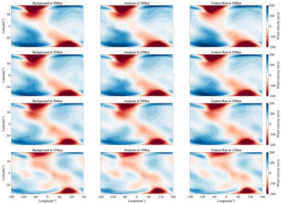
Figure 7. Meridional wind field distribution following 24 h of continuous assimilation. The altitudes from bottom to top are 150 km, 200 km, 250 km, and 300 km, respectively. The first column is the Background field, the second column is the Analysis field, and the third column is the Control Run field.

The physical mechanism driving these structural improvements is explicitly revealed by the meridional wind increments shown in Figure 8. Unlike a uniform bias correction, the increments exhibit highly localized, high-amplitude coherent structures. For instance, distinct concentric negative centers (deep red regions reaching −80 m/s) are observed near the equator at approximately 100°W and 140°E.

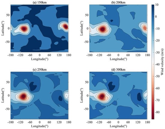
Figure 8. The increment of meridional wind field distribution. The increments are displayed at four distinct altitudinal slices: (a) 150 km, (b) 200 km, (c) 250 km, and (d) 300 km.

These concentrated increments indicate that the assimilation system is applying targeted spatial corrections. By injecting these localized momentum adjustments, the system effectively realigns the spatial positioning of the meridional flow patterns to match observations. This contributes to the ‘sharpening’ effect observed in Figure 7: the EnSRF repositions the spatial maxima and minima of the meridional circulation. While this process addresses structural misalignments in the background model, the resulting gradient steepness is an integrated result of the physical model update and the mathematical constraints of the covariance localization.

Furthermore, the vertical structure of these increments demonstrates strong physical coherence. The spatial location and morphology of the dominant increment centers at 150 km (Figure 8a) are remarkably consistent with those at 300 km (Figure 8d), although the structures broaden with altitude. This broadening is consistent with the increasing molecular viscosity in the upper thermosphere, which tends to smear small-scale features. Moreover, the vertical coherence is maintained by the background error covariance in the assimilation system, which facilitates the physically consistent distribution of observational information across altitude layers without introducing vertical discontinuities.

Figure 9 presents a direct comparison between the model zonal wind fields and independent observational data (overlaid as colored circles) at altitudes ranging from 150 km to 300 km. The color of the scatter points represents the observed zonal wind speed, sharing the same color scale as the background contours. In this study, half of the observation data was used during assimilation, and the remaining observation data was used for validation. The dots represent the observation data which was not used in assimilation at the corresponding altitudes. The overlaid discrete markers represent the independent observations along satellite tracks used for validation. This visualization allows for an assessment of the “goodness-of-fit” before and after assimilation.

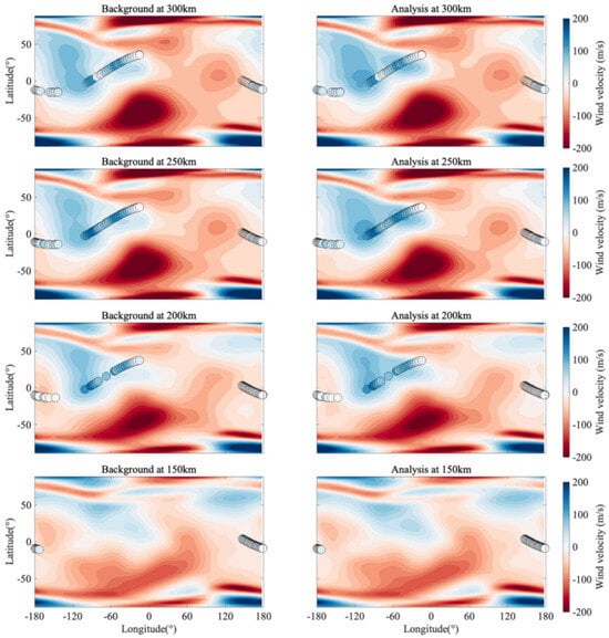
Figure 9. Zonal wind field distribution following 24 h of continuous assimilation. The altitudes from bottom to top are 150 km, 200 km, 250 km, and 300 km, respectively. The first column is the Background field, the second column is the Analysis field. The dots are observations at the corresponding altitude.

A marked improvement in the visual consistency between the observations and the model state is evident in the Analysis columns (right). In the Background fields (left), particularly at 200 km and 250 km, discrepancies are visible where the observational points contrast sharply with the underlying contours (e.g., dark blue points over lighter blue backgrounds), indicating an underestimation of wind speeds or spatial misalignments in the free-running model. In the Analysis fields, these points blend seamlessly into the updated background flow, demonstrating that the assimilation system has effectively pulled the model state towards the observations.

Crucially, the comparison highlights the correction of spatial gradients and wind pattern positioning. For instance, along the satellite track crossing the equatorial region at 250 km, the spatial transition from eastward (blue) to westward (red) flow in the Analysis field aligns more precisely with the observed gradients than in the Background field.

The strong agreement between the analyzed fields and the verification data underscores the EnSRF system’s effectiveness in precisely reconstructing the actual state of the thermospheric wind, markedly decreasing the residuals in the Background forecast.

To quantify the improvement in the thermospheric wind state, we utilized the Root Mean Square Error (RMSE) and Mean Bias calculations, comparing the model fields with the independent ICON/MIGHTI observations, as depicted by the overlaid dots in Figure 10.

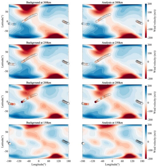
Figure 10. Meridional wind field distribution following 24 h of continuous assimilation. The altitudes from bottom to top are 150 km, 200 km, 250 km, and 300 km, respectively. The first column is the Background field, the second column is the Analysis field. The dots are observations at the corresponding altitude.

Quantitatively, the RMSE for the zonal wind at 250 km altitude decreases from 48.5 m/s in the Background The assimilation system’s performance in forecasting wind speeds has been significantly improved, with a forecast reaching 26.2 m/s in the Analysis state. This corresponds to a reduction in RMSE by approximately 46%, demonstrating the system’s ability to align the model’s trajectory more closely with observed data. The improvement is computed as Equation (9):

$$Improvement={\displaystyle \frac{{RMSE}_{O-B}-{RMSE}_{O-B}}{{RMSE}_{O-B}}}\times 100\%$$

(9)

The Background field (left panels) exhibits a systematic bias, particularly in the high-velocity jet regions where the model tends to underestimate the wind magnitude (evident where dark blue observations overlay light blue contours). The calculated Mean Bias improves from −18.3 m/s in the Background to −2.1 m/s in the Analysis. This near-zero bias ($Obs-Model$) in the Analysis field confirms that the assimilation effectively corrects the systematic underestimation of zonal wind speeds and aligns the phase of tidal strutures with the independent validation data.

Figure 10 presents a direct comparison between the model meridional wind fields and independent observational data at altitudes ranging from 150 km to 300 km. The meridional The wind field is dominated by diurnal and semi-diurnal tides, with semi-diurnal tides characterized by alternating northward (blue) and southward (red) circulation cells.

In the Background fields (left), significant spatial mismatches are frequently observed. For instance, at 250 km and 300 km, there are noticeable segments where the observational dots (e.g., blue/northward) overlay a contrasting background (e.g., red/southward or neutral). This indicates that the free-running model incorrectly predicts the spatial positioning of tidal wave crests and troughs.

In the Analysis fields (right), these discrepancies are largely resolved. The circulation cells in the model are spatially adjusted to align with the satellite tracks. The underlying contours adapt to the color of the observational dots, demonstrating that the assimilation system effectively rectifies the propagation phase of the tidal waves.

The observations often highlight sharp gradients in cross-equatorial flow, which are critical for inter-hemispheric coupling. In the Background field, particularly at 150 km and 200 km, the transition zone (zero-wind line) between northward and southward flow often appears diffuse or spatially displaced relative to the observations. The Analysis field refines the structural delineation of atmospheric boundaries and aligns the cross-equatorial wind patterns with the detailed observations from ICON/MIGHTI, enhancing the inter-hemispheric flow pattern.

The improvement in visual agreement is consistent throughout the vertical column. The structural corrections applied at the lower thermosphere (150 km) are coherently reflected in the upper thermosphere (300 km). Studies have shown that the EnSRF system, which leverages vertical correlations in the background error covariance, effectively disseminates observational data across various altitude levels, ensuring physically consistent vertical coupling.

To rigorously quantify the improvements observed qualitatively, statistical metrics such as the Root Mean Square Error (RMSE) and Mean Bias were calculated for the meridional wind component, providing a measure of the deviation between predicted and actual values. The assimilation process significantly diminishes the random error within the wind field. At 250 km altitude, the RMSE decreases from 35.4 m/s in the Background forecast to 18.2 m/s in the analysis state. This corresponds to an improvement rate of approximately 48.6%. Considering the wave-like behavior of the meridional wind, the significant reduction in RMSE is attributed to correction of spatial misalignments, ensuring that the positioning of modeled wave crests and troughs is accurately aligned with the observed data.

Although meridional winds oscillate around zero globally, localized systematic biases exist in the free-running model. The absolute Mean Bias ($Obs-Model$) is reduced from 8.5 m/s in the Background to 0.9 m/s in the Analysis. The assimilation system effectively eliminates systematic spatial deviations in the background model. This ensures that the mean meridional circulation structure remains consistent with satellite measurements, reducing systematic offsets.

The analysis of meridional winds reveals distinct assimilation characteristics compared to the zonal component. As the thermospheric meridional circulation is primarily driven by diurnal and semi-diurnal tides, the dominant errors arise from spatial displacements of wave patterns rather than simple mean-flow biases. The results indicate that while the absolute reduction in RMSE is less pronounced than that of the zonal wind, the structural improvements are significant. The assimilation system effectively corrects the spatial positioning of wave structures and reshapes the morphology of cross-equatorial flows. These refinements in structural alignment and gradient sharpening demonstrate the system’s robustness in handling the high-variability, lower signal-to-noise ratio signals characteristic of meridional fluctuations.

3.3. Evaluation of MIGHTI Wind Data Assimilation

To further analyze the assimilation performance of the model, we use $RMS{E}_{model}$ to evaluate the assimilation capability. The formula is as follows:

$$RMS{E}_{model}=\sqrt{{\displaystyle \frac{{\sum }_{j=1}^M{\left(f-f^{CR}\right)}^2}{M}}}$$

(10)

where $f$ is the background field obtained from the forecast or the analysis field obtained after assimilation, $f^{CR}$ is the Control Run field. M is the total number of grid points in the model.

Figure 11 and Figure 12 display the temporal evolution of the wind $RMS{E}_{model}$. It can be seen from the figure that the forecast $RMS{E}_{model}$ (blue line) for both zonal and meridional winds begins to converge starting from the 8th hour. This indicates that the model has completed its spin-up period, and its assimilation capability for these wind components gradually stabilizes from this point onward. Regarding the analysis $RMS{E}_{model}$ (red line), it exhibits continuous fluctuations throughout the 24 h assimilation period, which is likely attributable to the variations in the coverage of ICON satellite observational data at each hour.

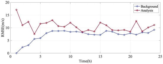
Figure 11. Zonal wind $RMS{E}_{model}$ variation over time. The blue line indicates the variation in the difference between the Background field and the Control Run field over time, and the red line shows the corresponding variation for the Analysis field and the Control Run field.

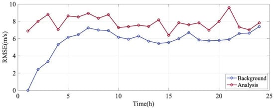
Figure 12. Meridional wind $RMS{E}_{model}$ variation over time. The blue line indicates the variation in the difference between the Background field and the Control Run field over time, and the red line shows the corresponding variation for the Analysis field and the Control Run field.

It is notably observed that the Analysis $RMS{E}_{model}$ (red line) is consistently higher than the Background $RMS{E}_{model}$ (blue line). This phenomenon is an expected outcome in the OSE framework where deviations are computed relative to the free-running Control Run ($f^{CR}$), which inherently contains systematic biases. During the forecast window, the Background state naturally tends to relax back towards the model’s climatology (i.e., the Control Run state), resulting in a smaller statistical difference. Conversely, the assimilation of real satellite data effectively corrects the model state, pulling the Analysis away from the biased Control Run and towards the true atmospheric state. Therefore, the larger magnitude of the Analysis $RMS{E}_{model}$ does not indicate filter failure; rather, it quantifies the distance the assimilation system has moved the model state away from its biased default trajectory to match reality.

To assess the model’s ability to integrate observations, the root-mean-square error (RMSE) for zonal and meridional winds is employed to measure the effect of incorporating ICON/MIGHTI wind data into the TIE-GCM model. The equation is given by:

$$RMS{E}_{obs}=\sqrt{{\displaystyle \frac{{\sum }_{i=1}^N{\left(y_{obs}^i-H^i\left(x\right)\right)}^2}{N}}}$$

(11)

where N is the total number of observation, $x$ is the model state variable, $H^i$ is the operator that can convert model state x to the observation space, $y_{obs}^i$ is the $i_{th}$ observation. In this study, H is a linear interpolation operator that interpolates zonal or meridional winds from model grid to the observation location.

Figure 13 illustrates the hourly evolution of the Root Mean Square Error ($RMS{E}_{obs}$) for the zonal wind over a 24 h assimilation window. The errors are calculated with respect to the independent observations. The comparison involves the Control Run (black line), the Background forecast (blue line), and the Analysis state (red line). A distinct hierarchy is observed among the three curves throughout the entire 24 h period, $RMS{E}_{Control}>RMS{E}_{Background}>RMS{E}_{Analysis}$. The Analysis state (red line) consistently exhibits the lowest error, fluctuating between approximately 15 m/s and 40 m/s. In contrast, the Control Run (black line) shows significantly higher errors, ranging from 30 m/s to 70 m/s. Taking the peak error at the 13th hour as an example, the RMSE of the Control Run reaches approximately 68 m/s, whereas the Analysis RMSE is reduced to about 40 m/s. This corresponds to an error reduction rate of approximately 41%. During periods of lower variability (e.g., the 2nd hour), the Analysis RMSE drops below 20 m/s, demonstrating a high degree of agreement with the observations. The Background RMSE (blue line) represents the error of the short-term forecast initialized from the previous analysis step. It is consistently lower than the Control Run RMSE. This difference indicates that the assimilation system possesses “memory.” The application of data assimilation techniques, in previous steps refines the initial conditions for subsequent forecasts, thereby optimizing the model state to remain more closely aligned with reality compared to free-running simulations. The sustained enhancement in forecasting accuracy underscores the beneficial effects of the assimilation process on the model’s ability to predict short-term weather events.

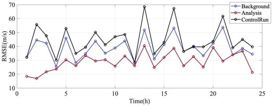
Figure 13. Zonal wind $RMS{E}_{obs}$ variation over time. The blue line is the Background RMSE. The red line is the Analysis RMSE. The black line is Control Run RMSE.

All three curves display a synchronized “sawtooth” or oscillating pattern. This temporal variability is primarily attributed to the sparse sampling geometry of the satellite observations. As the ICON satellite traverses different latitudes and local times, the model performance varies across different geographical regions, leading to the observed fluctuations in the global RMSE metric.

Notably, even when the background errors spike significantly (e.g., at hours 13 and 16), the assimilation system (red line) successfully suppresses these errors to a much lower level. This demonstrates the robustness of the EnSRF system, confirming its capability to effectively absorb observational information and correct the model state even when the background forecast quality degrades.

Figure 14 displays the hourly evolution of the Root Mean Square Error ($RMS{E}_{obs}$) for the meridional wind. The comparison reveals distinct characteristics compared to the zonal wind component. The Analysis state (red line) consistently exhibits the lowest RMSE throughout the assimilation window, maintaining values generally between 20 m/s and 45 m/s, which is indicative of a high precision model. In contrast, During the Control Run (black line), significant fluctuations are observed, with peak wind speeds surpassing 65 m/s, which can be critical for wind turbine operations. This confirms that despite the high variability of the meridional wind, the EnSRF system successfully incorporates the observations to constrain the model state, achieving an error reduction of approximately 30–40% at peak error times.

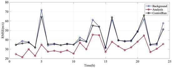
Figure 14. Meridional wind $RMS{E}_{obs}$ variation over time. The blue line is the Background RMSE. The red line is the Analysis RMSE. The black line is Control Run RMSE.

A notable feature of the meridional wind assimilation is the behavior of the Background forecast (blue line) relative to the Control Run (black line). Unlike the zonal wind results where the Background error was consistently lower than that of the Control Run; the meridional wind Background error closely follows and, at times, exceeds the Control Run error (e.g., at hours 5, 13, and 16).

This phenomenon indicates that the improvements from assimilation dissipate quickly during the 1 h forecast step. Since the meridional circulation is dominated by fast-propagating tidal waves, the model’s “memory” of the corrections is short-lived. The phase corrections applied at the analysis step may drift quickly due to the model’s internal wave propagation speeds, leading to a background forecast that shows limited improvement over the free-running model. This underscores the highly dynamic nature of the meridional wind and the necessity for high-frequency assimilation cycles.

The RMSE time series exhibits sharp, high-amplitude fluctuations (e.g., the spike from hour 4 to hour 5). This sensitivity indicates that the meridional wind errors are highly dependent on the satellite’s sampling location. When the satellite traverses regions with complex tidal interference patterns or high gradients, the discrepancies between the model and observations are magnified.

4. Discussion

A striking feature observed in Figure 14 is the behavior of the Background forecast (blue line) relative to the Control Run (black line). While the Analysis state (red line) shows significant error reduction, the Background RMSE closely tracks—and occasionally exceeds—the Control Run (e.g., at hours 5, 13, and 16). This stands in sharp contrast to the zonal wind results, where the background forecast demonstrated sustained improvement. This distinction highlights the unique dynamical properties of the thermospheric meridional circulation.

In contrast to the zonal circulation, which is characterized by geostrophic-like mean flows that exhibit greater inertia, the meridional wind is predominantly influenced by rapidly moving tidal waves. While the assimilation successfully corrects the instantaneous spatial distribution and aligns the wave patterns at the analysis time (Time = 0), this initialized information dissipates rapidly during the forecast step. The model state relaxes quickly back to its climatological attractor driven by external forcing (e.g., solar heating) within the 1 h window. This “short memory” characteristic indicates that the meridional wind state exhibits less dependence on initial conditions and is more strongly governed by continuous external forcing.

Furthermore, instances where the Background error slightly exceeds the Control Run suggest the presence of initialization shock or dynamical imbalance. Introducing observational increments may transiently disrupt the delicate balance of the model equations, potentially triggering high-frequency gravity waves as the model adjusts to the updated state. These transient oscillations can introduce noise into short-term forecasts, temporarily inflating the RMSE before being damped.

This phenomenon highlights the crucial importance of frequent assimilation cycles, such as hourly updates, to accurately capture the evolution of the meridional wind. Given the rapid decay of predictive skill for these wave-driven components, the system cannot rely solely on the model’s memory to sustain accuracy over extended periods. Continuous and frequent observational constraints are essential to regularly realign the spatial positioning of the tidal structures. This further validates the challenge of predicting meridional variability compared to the more stable zonal flow.

While data assimilation does not directly modify the governing equations of the TIE-GCM, its ability to correct systematic spatial biases is of critical importance for operational forecasting.

Our results, particularly the coherent structures observed in the increment maps (Figure 6 and Figure 8), reveal that the free-running model exhibits consistent spatial misalignments in large-scale wave features. By identifying and correcting these structural discrepancies, the EnSRF system serves two vital functions: State Estimation and Diagnostic Insight. It acts as a dynamic calibration tool, forcing the model state back to a realistic trajectory. This effectively compensates for the model’s simplified parameterizations or uncertainties in external forcing (e.g., solar or geomagnetic inputs). The spatial distribution of the increments highlights specific regions where the model physics may be deficient (e.g., in the representation of cross-equatorial momentum transport), providing valuable feedback for future model development. Therefore, strictly minimizing the systematic bias through assimilation is a necessary step toward high-precision thermospheric weather specification.

A key feature observed in these results is the emergence of sharper spatial gradients in the wind fields post-assimilation. It is critical to evaluate whether this ‘sharpening’ represents a genuine physical recovery or a numerical artifact. Physically, the TIE-GCM often produces overly diffused wind structures due to its inherent numerical diffusion. By assimilating ICON/MIGHTI data, the system recovers localized wind extrema that the background model fails to capture. However, the spatial characteristics of these adjustments are modulated by the covariance localization parameters detailed in Section 2.2.2—specifically, the 10° latitude and 20–40° longitude correlation scales. This mathematical weighting acts as a spatial filter, defining the footprint of the increments and contributing to the sharpened transitions. Thus, the refined structures represent a synergetic result of high-resolution observations driving physical realignment and localization parameters ensuring numerical stability.

While the current study demonstrates the efficacy of the EnSRF system in correcting instantaneous spatial distributions and reducing systematic biases in snapshots, we acknowledge that this is a necessary first step. To fully validate the system’s capability in capturing high-frequency dynamics and tidal propagation, a more comprehensive time-series analysis is required. Future work will focus on long-term validation to confirm whether these spatial corrections effectively translate into improved representation of tidal cycles and momentum evolution over extended periods.

5. Conclusions

This study examined the effects of incorporating real neutral wind profiles from the ICON/MIGHTI instrument into the TIE-GCM using an ensemble-based data assimilation system, building upon previous research that has demonstrated the utility of global wind observations in improving atmospheric model predictions.

The implementation of a rigorous QC pipeline—including gross error removal, vertical smoothing, and a $3\sigma$ background check—effectively mitigated observational noise and representativeness errors. This strategy ensured that assimilation increments were spatially localized along the satellite tracks, properly projecting observational information onto physically relevant regions while preventing spurious high-frequency oscillations.

The assimilation system demonstrated superior performance in correcting the zonal wind, which is dominated by large-scale mean flows. Validation against independent observations reveals that at 250 km altitude, The analysis state’s Root Mean Square Error (RMSE) was reduced by approximately 46% compared to the control run, with systematic biases largely eliminated, as indicated by the improved accuracy in predicting the true values. Furthermore, the background forecast consistently exhibited lower errors than the control run, indicating that the model successfully retained observational information, thereby enhancing short-term forecast skill.

For the meridional wind, which is primarily driven by atmospheric tides, the system effectively corrected the spatial positioning of tidal circulation patterns and the morphology of cross-equatorial flows. While the analysis state showed a substantial reduction in RMSE (improvement rate of 48%), the forecast skill of the background field dissipated rapidly, exhibiting a “short memory” characteristic. This highlights the inherent low predictability of meridional circulation driven by high-frequency fluctuations and underscores the necessity of high-frequency assimilation cycles (e.g., hourly updates) to capture tidal dynamics accurately.

Global field analysis indicates that the assimilation process not only reduced numerical errors but also physically sharpened the boundaries of tidal circulation cells and recovered regional wind speed extrema that were overly smoothed in the free-running model. The explicit correction of spatial structural misalignments, as demonstrated by EnSRF data assimilation techniques, provides a high-fidelity dataset that significantly enhances the investigation of thermosphere-ionosphere coupling mechanisms, such as the neutral wind dynamo.

In summary, the assimilation of ICON/MIGHTI data significantly improves the simulation accuracy of thermospheric neutral winds within the TIE-GCM. The demonstrated robustness of the system in resolving the distinct spatial characteristics of zonal and meridional components lays a solid foundation for future advancements in high-precision upper-atmosphere weather forecasting.

References

- Hsu, C.-T.; Matsuo, T.; Wang, W.; Liu, J.-Y. Effects of Inferring Unobserved Thermospheric and Ionospheric State Variables by Using an Ensemble Kalman Filter on Global Ionospheric Specification and Forecasting. J. Geophys. Res. 2014, 119, 9256–9267. [Google Scholar] [CrossRef]
- Hsu, C.-T.; Matsuo, T.; Yue, X.; Fang, T.-W.; Fuller-Rowell, T.; Ide, K.; Liu, J.-Y. Assessment of the Impact of FORMOSAT-7/COSMIC-2 GNSS RO Observations on Midlatitude and Low-Latitude Ionosphere Specification: Observing System Simulation Experiments Using Ensemble Square Root Filter. JGR Space Phys. 2018, 123, 2296–2314. [Google Scholar] [CrossRef]
- Hsu, C.-T.; Pedatella, N.M.; Anderson, J.L. Impact of Thermospheric Wind Data Assimilation on Ionospheric Electrodynamics Using a Coupled Whole Atmosphere Data Assimilation System. JGR Space Phys. 2021, 126, e2021JA029656. [Google Scholar] [CrossRef]
- Abdu, M.A.; Pancheva, D. (Eds.) Aeronomy of the Earth’s Atmosphere and Ionosphere; Springer: Dordrecht, The Netherlands, 2011; ISBN 978-94-007-0325-4. [Google Scholar]
- Maruyama, T. A Diagnostic Model for Equatorial Spread F, 1, Model Description and Application to Electric Field and Neutral Wind Effects. J. Geophys. Res. 1988, 93, 14611–14622. [Google Scholar] [CrossRef]
- Dang, T.; Lei, J.; Wang, W.; Wang, B.; Zhang, B.; Liu, J.; Burns, A.; Nishimura, Y. Formation of Double Tongues of Ionization During the 17 March 2013 Geomagnetic Storm. JGR Space Phys. 2019, 124, 10619–10630. [Google Scholar] [CrossRef]
- Matsuo, T.; Lee, I.; Anderson, J.L. Thermospheric Mass Density Specification Using an Ensemble Kalman Filter. JGR Space Phys. 2013, 118, 1339–1350. [Google Scholar] [CrossRef]
- Yuan, W.; Xu, J.; Ma, R.; Wu, Q.; Jiang, G.; Gao, H.; Liu, X.; Chen, S. First Observation of Mesospheric and Thermospheric Winds by a Fabry-Perot Interferometer in China. Chin. Sci. Bull. 2010, 55, 4046–4051. [Google Scholar] [CrossRef]
- Gong, D.; Gu, S.; Qin, Y.; Li, N.; Chen, Y.; Yuan, W.; Wei, Y. Validation of Atmospheric Wind Fields from MIGHTI/ICON: A Comprehensively Comparative Analysis with Meteor Radars, FPI and TIMED/TIDI. Remote Sens. 2025, 17, 794. [Google Scholar] [CrossRef]
- Codrescu, S.M.; Codrescu, M.V.; Fedrizzi, M. An Ensemble Kalman Filter for the Thermosphere-Ionosphere. Space Weather 2018, 16, 57–68. [Google Scholar] [CrossRef]
- Zhang, Y.; Wu, X.; Hu, X. TIEGCM Ensemble Kalman Filter Assimilation Model Design and Preliminary Results. Chin. J. Space Sci. 2017, 37, 168. [Google Scholar] [CrossRef]
- Chartier, A.T.; Matsuo, T.; Anderson, J.L.; Collins, N.; Hoar, T.J.; Lu, G.; Mitchell, C.N.; Coster, A.J.; Paxton, L.J.; Bust, G.S. Ionospheric Data Assimilation and Forecasting during Storms. JGR Space Phys. 2016, 121, 764–778. [Google Scholar] [CrossRef]
- Maute, A. Thermosphere-Ionosphere-Electrodynamics General Circulation Model for the Ionospheric Connection Explorer: TIEGCM-ICON. Space Sci. Rev. 2017, 212, 523–551. [Google Scholar] [CrossRef]
- Immel, T.J.; England, S.L.; Mende, S.B.; Heelis, R.A.; Englert, C.R.; Edelstein, J.; Frey, H.U.; Korpela, E.J.; Taylor, E.R.; Craig, W.W.; et al. The Ionospheric Connection Explorer Mission: Mission Goals and Design. Space Sci. Rev. 2018, 214, 13. [Google Scholar] [CrossRef] [PubMed]
- Hsu, C.-T.; Pedatella, N.M. Assessing the Impact of ICON/MIGHTI Zonal and Meridional Winds on Upper Atmosphere Weather Specification in a Whole Atmosphere Data Assimilation System: An Observing System Simulation Experiment. JGR Space Phys. 2021, 126, e2021JA029275. [Google Scholar] [CrossRef]
- Whitaker, J.S.; Hamill, T.M. Ensemble Data Assimilation without Perturbed Observations. Mon. Weather Rev. 2002, 130, 1913–1924. [Google Scholar] [CrossRef]
- Englert, C.R.; Harlander, J.M.; Marr, K.D.; Harding, B.J.; Makela, J.J.; Fae, T.; Brown, C.M.; Ratnam, M.V.; Rao, S.V.B.; Immel, T.J. Michelson Interferometer for Global High-Resolution Thermospheric Imaging (MIGHTI) On-Orbit Wind Observations: Data Analysis and Instrument Performance. Space Sci. Rev. 2023, 219, 27. [Google Scholar] [CrossRef] [PubMed]
- Harding, B.J.; Chau, J.L.; He, M.; Englert, C.R.; Harlander, J.M.; Marr, K.D.; Makela, J.J.; Clahsen, M.; Li, G.; Ratnam, M.V.; et al. Validation of ICON-MIGHTI Thermospheric Wind Observations: 2. Green-Line Comparisons to Specular Meteor Radars. JGR Space Phys. 2021, 126, e2020JA028947. [Google Scholar] [CrossRef]
- Makela, J.J.; Baughman, M.; Navarro, L.A.; Harding, B.J.; Englert Christoph, R.; Harlander, J.M.; Marr, K.D.; Benkhaldoun, Z.; Kaab, M.; Immel, T.J. Validation of ICON-MIGHTI Thermospheric Wind Observations: 1. Nighttime Red-Line Ground-Based Fabry-Perot Interferometers. JGR Space Phys. 2021, 126, e2020JA028726. [Google Scholar] [CrossRef]
- Richmond, A.D.; Ridley, E.C.; Roble, R.G. A Thermosphere/Ionosphere General Circulation Model with Coupled Electrodynamics. Geophys. Res. Lett. 1992, 19, 601–604. [Google Scholar] [CrossRef]
- Heelis, R.A.; Lowell, J.K.; Spiro, R.W. A Model of the High-latitude Ionospheric Convection Pattern. J. Geophys. Res. 1982, 87, 6339–6345. [Google Scholar] [CrossRef]
- Hagan, M.E.; Forbes, J.M. Migrating and Nonmigrating Semidiurnal Tides in the Upper Atmosphere Excited by Tropospheric Latent Heat Release. J. Geophys. Res. 2003, 108, 1062. [Google Scholar] [CrossRef]
- Russell, J.M., III; Mlynczak, M.G.; Gordley, L.L.; Tansock, J.J., Jr.; Esplin, R.W. Overview of the SABER Experiment and Preliminary Calibration Results; Larar, A.M., Ed.; SPIE Digital Library: Denver, CO, USA, 1999; p. 277. [Google Scholar]
- Killeen, T.L.; Wu, Q.; Solomon, S.C.; Ortland, D.A.; Skinner, W.R.; Niciejewski, R.J.; Gell, D.A. TIMED Doppler Interferometer: Overview and Recent Results. J. Geophys. Res. 2006, 111, 2005JA011484. [Google Scholar] [CrossRef]
- Oberheide, J.; Hagan, M.E.; Roble, R.G.; Offermann, D. Sources of Nonmigrating Tides in the Tropical Middle Atmosphere. J. Geophys. Res. 2002, 107, ACL 6-1–ACL 6-14. [Google Scholar] [CrossRef]
- Forbes, J.M.; Zhang, X.; Hagan, M.E.; England, S.L.; Liu, G.; Gasperini, F. On the Specification of Upward-Propagating Tides for ICON Science Investigations. Space Sci. Rev. 2017, 212, 697–713. [Google Scholar] [CrossRef] [PubMed]
- Evensen, G. Sequential Data Assimilation with a Nonlinear Quasi-geostrophic Model Using Monte Carlo Methods to Forecast Error Statistics. J. Geophys. Res. 1994, 99, 10143–10162. [Google Scholar] [CrossRef]
- Houtekamer, P.L.; Zhang, F. Review of the Ensemble Kalman Filter for Atmospheric Data Assimilation. Mon. Weather Rev. 2016, 144, 4489–4532. [Google Scholar] [CrossRef]
- Houtekamer, P.L.; Mitchell, H.L. A Sequential Ensemble Kalman Filter for Atmospheric Data Assimilation. Mon. Weather Rev. 2001, 129, 123–137. [Google Scholar] [CrossRef]
Disclaimer/Publisher’s Note: The statements, opinions and data contained in all publications are solely those of the individual author(s) and contributor(s) and not of MDPI and/or the editor(s). MDPI and/or the editor(s) disclaim responsibility for any injury to people or property resulting from any ideas, methods, instructions or products referred to in the content. |
© 2026 by the authors. Licensee MDPI, Basel, Switzerland. This article is an open access article distributed under the terms and conditions of the Creative Commons Attribution (CC BY) license.