A New Method for Detecting Automated Mapping Anomalies in Himalayan Glacial Lakes from Satellite Images

Highlights

What is the main finding?

• The proposed Evolutionary Feature Gaussian Process (EF-GP) can effectively identify anomalous observations arising from deviations in glacial lake boundary recognition caused by the interference of clouds, snow, and terrain shadows in remote sensing imagery, while preserving the genuine evolutionary processes of the glacial lakes.

What is the implication of the main finding?

• The ‘EF-GP’ proposed in this study substantially enhances the quality of automated remote-sensing mapping of glacial lakes, enabling the development of high-quality, long-term glacial-lake datasets and providing reliable support for large-scale monitoring.

Abstract

The retreat of glaciers has accelerated the expansion of glacial lakes, heightening the risk of outburst floods. Satellite remote sensing provides a crucial means for monitoring these lakes. Yet, artifacts caused by cloud cover and shadows inevitably persist even after preprocessing, compromising the reliability of large-scale automated analyses. However, the conventional approach views such data noise merely as an obstacle to be removed. The critical research gap lies in the lack of systematic methods to identify and filter out anomalies arising from unavoidable interferences actively. To address this, we propose a Gaussian process anomaly detection method that incorporates features of glacial lake evolution. By modeling how lakes change over time and establishing confidence intervals, this study effectively detects anomalies in automatically identified glacial lakes from remote sensing imagery. Analysis of typical Himalayan glacial lakes demonstrates that this method achieves an F1-score of 0.95, significantly improving the precision of remote sensing datasets. Overall, this research provides valuable technical support for developing high-quality glacial lake datasets and for automating lake monitoring.

1. Introduction

Glacial lakes, formed by glacial processes, are crucial water bodies that significantly influence hydrological cycles in high-mountain regions [1]. As global warming accelerates glacier retreat [2,3,4], both the number and volume of glacial lakes have been increasing [5,6,7]. These lakes’ dam structures can become unstable due to processes triggered directly—such as rising lake levels caused by abnormal snowmelt, rainfall, or rapid glacier retreat—or indirectly, such as ice or rock avalanches into the lake or dam erosion [8,9]. Such instabilities heighten the risk of glacial lake outburst floods (GLOFs). Such floods have caused substantial loss of life, damage to infrastructure [10], and pose serious threats to the safety of infrastructure, residents, and property in high-altitude regions [11,12,13].

Satellite remote sensing has become a critical tool for real-time monitoring of glacial lakes in remote, mountainous areas [14,15]. Data from satellites like Landsat and Sentinel are commonly used to analyze the distribution, areal extent, and water volume of these lakes [16,17,18]. Recent advances in deep learning algorithms have greatly improved the automated identification of glacial lake boundaries [19,20], providing effective methods for creating long-term datasets on lake-area dynamics [21]. This technology enables automated feature extraction and learning from remote sensing images to detect water bodies [1,22], supporting disaster risk assessment and early warning systems for glacial lakes [23]. However, cloud, snow, and terrain shadows in optical remote sensing images can lead to misclassification or omission of glacial lake boundaries [24,25], thereby reducing the accuracy of automated glacial lake detection. These datasets often exhibit anomalies that distort observed lake-area trends, making it challenging to identify signals, including lake-level changes driven by dam operations, water balance, or other factors. Therefore, removing these anomalies from automatically generated data is essential to improve the reliability of glacial lake datasets and support scientific research.

Time series anomaly detection techniques have proven effective in identifying data change points and irregular fluctuations [26,27]. Removing anomalies can significantly improve data reliability [28], thereby offering new solutions for automated glacial lake monitoring. Statistical threshold techniques, such as the Hampel filter [29], leverage the data distribution to detect outliers efficiently [30]. For example, Chang et al. [31] used a Hampel filter to smooth the series of reservoir water extent across satellite platforms, removing outliers. These methods are commonly used in hydrological research [32] due to their straightforwardness and computational efficiency [33]. However, they often create long-term trends or seasonal patterns, which can result in misclassification or the overlooking of anomalies [34]. To improve detection performance, researchers decompose time series to separate trends and seasonal effects [35], then analyze the residuals for anomalies, thereby better capturing periodic variations. The ARIMA (Auto Regressive Integrated Moving Average) model is also widely applied in water quality analysis [36]. However, its success depends on proper parameter settings, as incorrect choices can misinterpret regular seasonal changes as anomalies [37]. Machine learning techniques such as the Local Outlier Factor (LOF) [38] and Long Short-Term Memory (LSTM) networks [39] have demonstrated high performance in detecting environmental anomalies. For instance, Mokua et al. [40] employed the LOF algorithm to identify outliers in water quality data, while Arathy et al. [41] applied an LSTM autoencoder for anomaly detection in flow rate time series.

Nevertheless, their effectiveness varies depending on data conditions [42], and they often lack interpretability [43]. Although they are widely applied in hydrometeorological and environmental monitoring, research specifically on high-mountain glacial lake monitoring remains limited.

This study presents a Gaussian process-based anomaly detection method that leverages features of glacial lake evolution to enhance remote sensing monitoring. Our goals are: (1) to develop a reliable anomaly detection algorithm for Himalayan lakes and evaluate their performance; (2) to create a high-accuracy time series dataset for monitoring glacial lakes. This study has the potential to offer a new approach to creating large-scale glacial lake datasets and provides an effective way to monitor glacial lakes.

2. Study Area and Data

2.1. Case Study Area

The study focuses on the eastern central Himalayas (Figure 1), situated along orbit 139/041 of the Worldwide Reference System. Covering 31,700 km², this region has 1489.96 km² of glaciers. Accelerated glacier melting due to climate change has led to the formation of new glacial lakes and the expansion of existing glacial lakes, increasing the risk of GLOFs. Previous GLOF events in this area, as documented by Nie et al. [44], have had considerable effects on downstream communities.

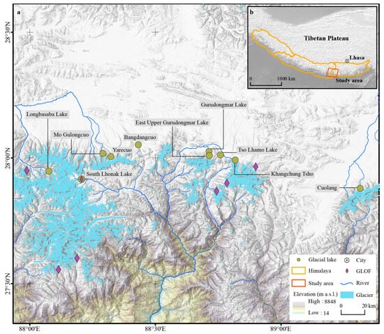
Figure 1. Study area location: (a) Map showing the distribution of glacier lakes included in the study. (b) The position of the case study area within the Himalayas.

Our study analyzes 10 representative moraine-dammed lakes within the study area (Table 1) for model training and validation. These lakes are grouped by size and types: the first group includes glacier-contact lakes larger than 1.40 km², such as Longbasaba Lake (1.75 km²), South Lhonak Lake (1.42 km²), and Khangchung Tsho (1.91 km²). These lakes have expanded significantly, with South Lhonak Lake experiencing a partial outburst in October 2023 [45]. The second group consists of glacier-contact lakes with areas less than 1.40 km², including East Upper Gurudongmar Lake (EUG Lake, 1.34 km²), Bangdangcuo (1.03 km²), and Cuolang (0.60 km²). These lakes have mostly remained stable, although EUG Lake and Bangdangcuo have recently shown slight expansion. The third group includes glacier-non-contact lakes, such as Gurudongmar Lake (1.13 km²), Tso Lhamo Lake (1.07 km²), Yarecuo (0.42 km²), and Mo Gulongcuo (0.56 km²), which have been relatively stable during the study period.

Table 1. Basic parameters of ten representative glacial lakes.

Name	Lake Type	Area in 2024 (km2)	Status
Longbasaba Lake	Glacier-contact	1.75	Expanding
South Lhonak Lake	Glacier-contact	1.42	Expanding and outburst
Khangchung Tsho	Glacier-contact	1.91	Expanding
EUG Lake	Glacier-contact	1.34	Slightly increase
Bangdangcuo	Glacier-contact	1.03	Slightly increase
Cuolang	Glacier-contact	0.60	Stable
Gurudongmar Lake	Glacier-non-contact	1.13	Stable
Tso Lhamo Lake	Glacier-non-contact	1.07	Stable
Yarecuo	Glacier-non-contact	0.42	Stable
Mo Gulongcuo	Glacier-non-contact	0.56	Stable

2.2. Data

A total of 89 satellite images from Landsat 5/7–9, collected between 1988 and 2024, were used to create a long-term dataset for 10 glacial lakes using an automated lake mapping method. All images are automatically selected and downloaded, filtering for cloud cover less than 30%. The data helps train anomaly detection algorithms, generating a high-quality dataset for monitoring changes in glacial lakes. The images consist of 56.1% from Landsat 8, 22.5% from Landsat 9, 16.9% from Landsat 5, and 4.5% from Landsat 7 (Figure 2a). Most images were acquired after 2020 (48.3%), followed by 2011 to 2020 (30.3%), 16.9% before 2000, and only 4.5% from 2001 to 2010 (Figure 2b). Most images were taken in autumn (68.5%) and summer (25.8%), while winter and spring each account for less than 4% (Figure 2c). October had the highest number of images (26), followed by November (23), while the months from June to September contributed 35 images overall (Figure 2d). An autumn period is ideal for examining longer-term changes because it is drier and less cloudy, whereas including other months will show seasonal fluctuations. Thus, this study primarily uses autumn and high-quality summer images to minimize the effects of seasonal changes and snow cover on the identification of glacial lake boundaries, thereby supporting the development of a comprehensive glacial lake database for further research.

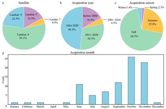
Figure 2. Statistics on Landsat satellite remote sensing imagery used in the study.

In any satellite image, a scene was considered a “valid observation” for a specific glacial lake and processed by the U-Net model for area extraction only if at least part of the lake was partially visible. If the lake was entirely obscured by clouds or shadows on that date, it was recorded as “no data.” As a result, the final number of observations varies across lakes, reflecting the number of images in which each lake could be processed algorithmically within the time series (Table 2). Table 2 summarizes the number of valid observations for the 10 studied glacial lakes and provides the calculated percentage of data loss due to complete obscuration by clouds, shadows, and similar interferences.

Table 2. Valid samples of glacial lakes observed via satellite.

Name	Number of Valid Samples	Total Observations	Percentage of Valid Observations
Longbasaba Lake	67	89	75.28%
South Lhonak Lake	58	89	65.17%
Khangchung Tsho	66	89	74.16%
EUG Lake	59	89	66.29%
Bangdangcuo	72	89	80.90%
Cuolang	49	89	55.06%
Gurudongmar Lake	69	89	77.53%
Tso Lhamo Lake	65	89	73.03%
Yarecuo	72	89	80.90%
Mo Gulongcuo	71	89	79.78%

3. Methods

This study presents an anomaly detection method, Evolutionary Feature Gaussian Process (EF-GP; Figure 3), designed to analyze the evolution of glacial lakes. The approach builds confidence intervals using Gaussian process modeling and incorporates three constraints based on the evolution of glacial lakes. This enhances the ability to distinguish between glacial lake outburst events and anomalous lake mapping, thereby significantly increasing the accuracy of glacial lake area time series.

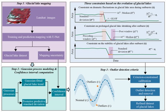
Figure 3. Flowchart of the Evolutionary Feature Gaussian Process for identifying anomalies in glacial lakes.

3.1. Automated Mapping of Glacial Lakes Using Remote Sensing

This research utilizes the U-Net deep learning architecture to automatically delineate glacial lakes [46,47], achieving an accuracy exceeding 90% in the Himalayan region [48]. The model architecture and processing pipeline are based on the framework of Zhang et al. [48], which has shown strong performance in the Himalayan region, with key metrics including precision (0.88), recall (0.96), F1-score (0.92), and IoU (0.84). The specific steps are as follows:

A total of 35 Landsat 8 images were used as training data. An interactive mapping tool assisted in labeling glacial lakes within these images [4,49]. This tool enabled users to select the area of interest (AOI) and produce an NDWI histogram. Users could then fine-tune the threshold to identify water bodies, ensuring the labels are reliable. The images and their labels were later split into 12,388 training samples, each measuring 512 × 512 pixels.

The model’s input consists of six Landsat 8 bands: Blue, Green, Red, NIR, SWIR1, and SWIR2. It is trained using the PyTorch (version 1.13.1) framework with the Adam optimizer, starting with a learning rate of 1 × 10⁻⁴ and a batch size of 8 over 200 epochs. After training, the model is applied to detect glacial lakes and generate data for anomaly detection.

To improve the robustness and transferability of the well-trained U-Net model, all Landsat raw images have been converted from digital number values to top-of-atmosphere reflectance.

3.2. Gaussian Process Modeling and Confidence Interval Construction

The Gaussian Process (GP) [50] is a non-parametric supervised learning approach based on Bayesian principles, which effectively minimizes noise and reconstructs the latent function underlying the data [51,52]. It is commonly applied in remote sensing data analysis [53,54]. In this study, the GP is used to model the time series of glacial lakes. Its key benefits include: (1) accurately capturing the evolution and long-term trends of glacial lakes; (2) distinguishing between minor fluctuations and rapid changes; and (3) providing a trustworthy measure of uncertainty through the posterior predictive standard deviation [55], which aids in establishing confidence intervals for anomaly detection.

3.2.1. Gaussian Process Modeling

This study uses the GP to model the time series trend of glacial lake areas ${\mathrm{D}}_{\mathrm{i}} = \left\{{\mathrm{x}}_{\mathrm{i}},{\mathrm{y}}_{\mathrm{i}},{\mathrm{\epsilon }}_{\mathrm{i}}\right\}$, $\mathrm{i} \in [1,\mathrm{n}]$, where ${\mathrm{x}}_{\mathrm{i}}$ denotes the temporal features of the glacial lake area changes, ${\mathrm{y}}_{\mathrm{i}}$ is the glacial lake area, and ${\mathrm{\epsilon }}_{\mathrm{i}}$ denotes the mapping uncertainty.

Here, ${\mathrm{x}}_{\mathrm{i}}$ is a continuous variable based on the image acquisition date, indicating the passage of time. For each glacial lake, we start by calculating the number of days since a fixed baseline date—the earliest date in that lake’s dataset—denoted as ${\mathrm{t}}_{\mathrm{i}}$ (in days). To ensure stable model fitting, we then standardize ${\mathrm{t}}_{\mathrm{i}}$ for each lake separately.

$${\mathrm{x}}_{\mathrm{i}}={\displaystyle \frac{({\mathrm{t}}_{\mathrm{i}}-{ \mathrm{\mu }}_{\mathrm{t}})}{{\mathrm{\sigma }}_{\mathrm{t}}}}$$

(1)

where ${\mathrm{\mu }}_{\mathrm{t}}$ and ${\mathrm{\sigma }}_{\mathrm{t}}$ represent the mean and standard deviation calculated from the lake’s specific ${\mathrm{t}}_{\mathrm{i}}$ values.

In this study, we develop an individual GP model for each glacial lake, treating each lake’s time series independently. In practice, each lake’s area data is loaded, its time axis is standardized, and a GP with a composite kernel is fitted exclusively to that lake’s data. Each lake has customized hyperparameters, including the length scale and signal variance, optimized by maximizing the marginal likelihood for that particular series.

The uncertainty in lake mapping (${\mathrm{\epsilon }}_{\mathrm{i}}$) was estimated using an improved Hanshaw’s function [18,56]. The equation is provided below:

$${\mathrm{\epsilon }}_{\mathrm{i}}= ({\displaystyle \frac{\mathrm{P}}{\mathrm{G}}}- {\mathrm{N}}_{\mathrm{Inner}}) \times 0.6872 \times {\displaystyle \frac{{\mathrm{G}}^2}{2}}$$

(2)

This method assumes that measurement errors for the area follow a normal distribution, with a 68.72% confidence interval at 1σ. In this context, P stands for the perimeter of the glacial lake, G indicates the spatial resolution of the imagery (79 m for Landsat 1–3, 30 m for Landsat 5–9, 10 m for Sentinel–2, and 3 m for Planet), and N_Inner represents the number of inner nodes in the lake’s vector boundary.

The modeling process is outlined as follows:

(1)

Kernel function:

$${\mathrm{k}}_{\mathrm{f}}\left({\mathrm{x}}_{\mathrm{i}},{\mathrm{x}}_{\mathrm{j}}\right) = {\mathrm{\sigma }}_{\mathrm{f}}^2\exp \left(-{\displaystyle \frac{{\left({\mathrm{x}}_{\mathrm{i}}-{\mathrm{x}}_{\mathrm{j}}\right)}^2}{2{\mathrm{\iota }}^2}}\right)$$

(3)

where ${\mathrm{\sigma }}_{\mathrm{f}}^2$ is the signal variance, and $\mathrm{\iota }$ is the length scale.

(2)

Covariance matrix structure:

$${\mathrm{K}}_{\mathrm{y}}={\left[{\mathrm{k}}_{\mathrm{f}}\left({\mathrm{x}}_{\mathrm{i}},{\mathrm{x}}_{\mathrm{j}}\right)\right]}_{\mathrm{i},\mathrm{j}=1}^{\mathrm{N}} +{\mathrm{\sigma }}_{\mathrm{n}}^2{\mathrm{I}}_{\mathrm{n}}$$

(4)

where ${\mathrm{\sigma }}_{\mathrm{n}}^2$ is the noise variance, and ${\mathrm{I}}_{\mathrm{n}}$ represents the $\mathrm{n} \times \mathrm{n}$ identity matrix.

(3)

Hyperparameter estimation:

The hyperparameters ${\mathrm{\sigma }}_{\mathrm{f}}^2$, $\mathrm{\iota }$ and ${\mathrm{\sigma }}_{\mathrm{n}}^2$, are estimated by maximizing the log-likelihood function:

$$\mathrm{logp}\left(\mathrm{Y}|\mathrm{X}\right) = -{\displaystyle \frac{1}{2}}{\mathrm{Y}}^{\mathrm{T}}{\mathrm{K}}_{\mathrm{y}}^{-1}\mathrm{Y} -{\displaystyle \frac{1}{2}}\log |{\mathrm{K}}_{\mathrm{y}}| -{\displaystyle \frac{\mathrm{n}}{2}}\log \left(2\mathrm{\pi }\right)$$

(5)

where $\mathrm{p}\left(\mathrm{Y}|\mathrm{X}\right)$ is the conditional probability of observing the output matrix $\mathrm{Y}$ given the input $\mathrm{X}$,$\mathrm{X} ={ \left[{\mathrm{x}}_1,\cdots ,{\mathrm{x}}_{\mathrm{n}}\right]}^{\mathrm{T}}$ and $\mathrm{Y} ={ \left[{\mathrm{y}}_1,\cdots ,{\mathrm{y}}_{\mathrm{n}}\right]}^{\mathrm{T}}$.

(4)

Prediction computation:

Calculate the estimated glacial lake area (${\widehat{\mathrm{y}}}_{\mathrm{i}}$):

$${\widehat{\mathrm{y}}}_{\mathrm{i}} ={ \mathrm{k}}_{\mathrm{i}}^{\mathrm{T}}{\mathrm{K}}_{\mathrm{y}}^{-1}\mathrm{Y}$$

(6)

where ${\mathrm{k}}_{\mathrm{i}}={\left[\mathrm{k}\right({\mathrm{x}}_{\mathrm{i}},{\mathrm{x}}_1),...,\mathrm{k}({\mathrm{x}}_{\mathrm{i}},{\mathrm{x}}_{\mathrm{n}}\left)\right]}^{\mathrm{T}}$.

Posterior predictive uncertainty:

$$\mathrm{\sigma }\left({\mathrm{x}}_{\mathrm{i}}\right) = \sqrt{\mathrm{k}\left({\mathrm{x}}_{\mathrm{i}},{\mathrm{x}}_{\mathrm{i}}\right)-{\mathrm{k}}_{\mathrm{i}}^{\mathrm{T}}{{{\mathrm{K}}_{\mathrm{y}}}^{-1}\mathrm{k}}_{\mathrm{i}}}$$

(7)

3.2.2. Creating Confidence Intervals

Based on GP modeling, the total uncertainty ${\mathrm{U}}_{\mathrm{i}}$ of the ith sample in this study is defined as the sum of the model’s posterior-prediction uncertainty and mapping uncertainty.

$${\mathrm{U}}_{\mathrm{i}}=\sqrt{{\mathrm{\sigma }}^2({\mathrm{x}}_{\mathrm{i}})+{{\mathrm{\epsilon }}_{\mathrm{i}}}^2}$$

(8)

The confidence interval for the ith glacial lake area is denoted as CI_i and can be expressed as:

$${\mathrm{CI}}_{\mathrm{i}} = [{\widehat{\mathrm{y}}}_{\mathrm{i}} - {\mathrm{U}}_{\mathrm{i}},{\widehat{\mathrm{y}}}_{\mathrm{i}} + {\mathrm{U}}_{\mathrm{i}}]$$

(9)

3.3. Criteria for Detecting Anomaly Values

Based on the confidence interval, the observed values of glacial lake area, ${\mathrm{y}}_{\mathrm{i}}$, can be categorized into three groups. These categories are: (1) ${\mathrm{C}}_1$ (above the upper confidence interval bound), which includes expanding glacial lake areas potentially caused by faster glacier melting, heavy rainfall, or overestimations due to cloud and snow interference in remote sensing images. (2) ${\mathrm{C}}_2$ (within the confidence interval), indicating typical natural fluctuations under normal climate conditions. (3) ${\mathrm{C}}_3$ (below the lower bound), where lake area reductions might be caused by mapping errors such as cloud shadowing or actual decreases resulting from events like GLOFs. This research identified the glacial lake areas in ${\mathrm{C}}_1$ and ${\mathrm{C}}_3$ as anomalous, while those in ${\mathrm{C}}_2$ were considered normal.

$${\mathrm{C}}_1=\left\{\mathrm{i} | {\mathrm{y}}_{\mathrm{i}} > {\widehat{\mathrm{y}}}_{\mathrm{i}}+{ \mathrm{U}}_{\mathrm{i}}\right\}$$

(10)

$${\mathrm{C}}_2=\left\{\mathrm{i} | {\widehat{\mathrm{y}}}_{\mathrm{i}}-{\mathrm{U}}_{\mathrm{i}} \le {\mathrm{y}}_{\mathrm{i}} \le {\widehat{\mathrm{y}}}_{\mathrm{i}}+{\mathrm{U}}_{\mathrm{i}}\right\}$$

(11)

$${\mathrm{C}}_3=\left\{\mathrm{i} | {\mathrm{y}}_{\mathrm{i}} < {\widehat{\mathrm{y}}}_{\mathrm{i}}-{\mathrm{U}}_{\mathrm{i}}\right\}$$

(12)

The sudden decrease in area caused by GLOFs is often mistaken for an anomaly. The study proposes three criteria to distinguish genuine outburst events from mapping errors, with a primary focus on the changes observed in glacial lakes following an outburst. These criteria include:

(1)

Constraint on dramatic fluctuations in glacial lake area during outbursts

Outburst events rapidly reduce the area of glacial lakes. For a specific value ${\mathrm{y}}_{\mathrm{i}}$, the historical window ${\mathrm{H}}_{\mathrm{i}}^{\mathrm{pre}}$, covering the range ${\{\mathrm{y}}_{\mathrm{i}-5},\dots ,{\mathrm{y}}_{\mathrm{i}-1}\}$, corresponds to the period {${\mathrm{x}}_{\mathrm{i}-5},\dots ,{\mathrm{x}}_{\mathrm{i}-1}$}. Since most glacial lakes have about 50–70 data points, we tested window sizes from 3 to 7 points. A window size of 5 provided the best balance between detection accuracy and false-positive rate on our training data and was selected as the optimal parameter.

The following criteria differentiate them.

$${\displaystyle \frac{{\mathrm{M}}_{\mathrm{i}}^{\mathrm{pre}}-{\mathrm{y}}_{\mathrm{i}}}{{\mathrm{\sigma }}_{\mathrm{i}}^{\mathrm{pre}}}} >{ \mathrm{\theta }}_{\mathrm{d}}$$

(13)

where ${\mathrm{M}}_{\mathrm{i}}^{\mathrm{pre}}$ represents the median of the historical window, ${\mathrm{\sigma }}_{\mathrm{i}}^{\mathrm{pre}}$ is the standard deviation, and ${\mathrm{\theta }}_{\mathrm{d}}$ is the threshold for dramatic fluctuations in glacial lake area.

(2)

Constraint on prolonged glacial lake shrinking after outburst

After the outburst, the lake area stays relatively low for a prolonged period. For the observed value ${\mathrm{y}}_{\mathrm{i}}$, a post-window ${\mathrm{H}}_{\mathrm{i}}^{\mathrm{post}}$ was defined as $\left\{{\mathrm{y}}_{\mathrm{i}}, \dots ,{ \mathrm{y}}_{\mathrm{i}+4}\right\}$. This corresponds to the range from a time span of $\left\{{\mathrm{x}}_{\mathrm{i}}, \dots , {\mathrm{x}}_{\mathrm{i}+4}\right\}$. The formula is given below:

$${\displaystyle \frac{{\mathrm{M}}_{\mathrm{i}}^{\mathrm{pre}}-{\mathrm{M}}_{\mathrm{i}}^{\mathrm{post}}}{{\mathrm{M}}_{\mathrm{i}}^{\mathrm{pre}}}} > {\mathrm{\theta }}_{\mathrm{l}}$$

(14)

where ${\mathrm{M}}_{\mathrm{i}}^{\mathrm{post}}$ represents the median of the historical window, and ${\mathrm{\theta }}_{\mathrm{l}}$ is the threshold for prolonged glacial lake shrinkage.

(3)

Constraint on the stability of glacial lakes after outburst

The glacial lake’s area shows minimal change after the outburst. The discrimination formula is provided below:

$${\mathrm{\sigma }}_{\mathrm{i}}^{\mathrm{post}} <{ \mathrm{\theta }}_{\mathrm{b}}$$

(15)

where ${\mathrm{\sigma }}_{\mathrm{i}}^{\mathrm{post}}$ represents the standard deviation of the post window, and ${\mathrm{\theta }}_{\mathrm{b}}$ is the threshold for the stability of glacial lakes.

If all the predefined conditions are satisfied, the sample is identified as the outburst time (${\mathrm{a}}_{\mathrm{i}}$ = outburst); otherwise, it is classified as an anomalous value (${\mathrm{a}}_{\mathrm{i}}$ = outlier).

3.4. Parameter Tuning and Performance Assessment

To evaluate the EF-GP algorithm, reference labels were manually created by visually examining satellite images. For each timestep across the ten glacial lakes’ area time series, the corresponding image was reviewed, and any observations affected by cloud cover, shadows from clouds or terrain, or seasonal ice and snow were marked as anomalous. All remaining observations were categorized as normal. Confirmed outburst events, which represent real physical changes, were included in the normal class when calculating detection metrics.

This study employs a grid search to identify the optimal parameter combination within the specified range (Table 3). Detection performance is evaluated using three metrics: precision (P), recall (R), and the F1-score (F). The combination with the highest F1-score is chosen as the optimal solution. The formulas for each metric are provided below.

$$\mathrm{P}={\displaystyle \frac{\mathrm{TP}}{\mathrm{TP}+\mathrm{FP}}}$$

(16)

$$\mathrm{R}={\displaystyle \frac{\mathrm{TP}}{\mathrm{TP}+\mathrm{FN}}}$$

(17)

$$\mathrm{F}={\displaystyle \frac{2\times \mathrm{R}\times \mathrm{P}}{\mathrm{R}+\mathrm{P}}}$$

(18)

Table 3. Parameter range for candidates in this study.

Parameters	Predefined Ranges
Threshold for dramatic fluctuations in glacial lake area (${\mathrm{\theta }}_{\mathrm{d}}$)	[1, 2, 3, 4, 5]
Threshold for prolonged glacial lake shrinkage (${\mathrm{\theta }}_{\mathrm{l}}$)	[0.05, 0.1, 0.15, 0.2, 0.25]
Threshold for the stability of glacial lakes (${\mathrm{\theta }}_{\mathrm{b}}$)	[0.05, 0.1, 0.15, 0.2, 0.25]

TP stands for true positives (normal samples correctly identified as such), TN is true negatives (outliers correctly identified as outliers), FP is false positives (outliers incorrectly identified as normal samples), and FN is false negatives (normal samples incorrectly identified as outliers).

This study aims to improve detection accuracy through an adaptive iterative optimization process that includes: (1) removing confirmed anomaly data points; (2) reconstructing the GP model with the remaining data; and (3) repeating these steps until no additional anomalies are found or until 20 iterations are reached.

Six glacial lakes—Longbasaba Lake, Mo Gulongcuo, Yarecuo, Tso Lhamo Lake, Bangdangcuo, and Gurudongmar Lake—were used as the training dataset for threshold optimization, utilizing grid search over specified ranges. Four additional lakes—Cuolang, EUG Lake, Khangchung Tsho, and South Lhonak Lake—served as the validation set for comparison. The experiments used the Hampel statistical method and the ARIMA time-series model to evaluate the performance of the EF-GP algorithm.

4. Results

4.1. Model Training Accuracy

The model’s performance was evaluated using 625 predefined threshold combinations, and the best threshold is listed in Table 4.

Table 4. Optimal parameter configuration.

Parameters	Optimal Threshold
Threshold for dramatic fluctuations in glacial lake area (${\mathrm{\theta }}_{\mathrm{d}}$)	3.0
Threshold for prolonged glacial lake shrinkage (${\mathrm{\theta }}_{\mathrm{l}}$)	0.1
Threshold for the stability of glacial lakes (${\mathrm{\theta }}_{\mathrm{b}}$)	0.1

The training outcomes highlight the model’s robust detection abilities (Table 5). The F1-score exceeds 0.90 across all samples, reaching a peak of 0.96. Both precision (0.92–1.00) and recall (0.92–1.00) remain consistently high, demonstrating the model’s reliable anomaly detection with a low false positive rate.

Table 5. Evaluating the metrics of the EF-GP.

Glacial Lake Name	Precision	Recall	F1-Score
Longbasaba Lake	0.97	0.92	0.94
Mo Gulongcuo	0.98	0.93	0.95
Yarecuo	0.98	0.95	0.96
Tso Lhamo Lake	1.00	0.92	0.96
Bangdangcuo	0.93	0.98	0.96
Gurudongmar Lake	0.92	1.00	0.96

4.2. Model Validation and Application

The evaluation on the validation dataset demonstrates excellent ability to identify anomalies in glacial lake areas, significantly enhancing the accuracy of long-term monitoring of glacial lake changes.

In the Cuolang glacial lake time series (Figure 4a), 12 out of 49 anomalies were detected, achieving 92% recall and an F1-score of 0.95. After removing anomalies from 1988 to 2024, the average lake area remained stable at 0.57 km². The optimized model effectively identified the 2013 anomaly (0.16 km²) and six additional anomaly events between 2015 and 2023. Without removing anomalies, the trend in the lake area appears blurry; however, after excluding anomalies, it shows a gradual increase.

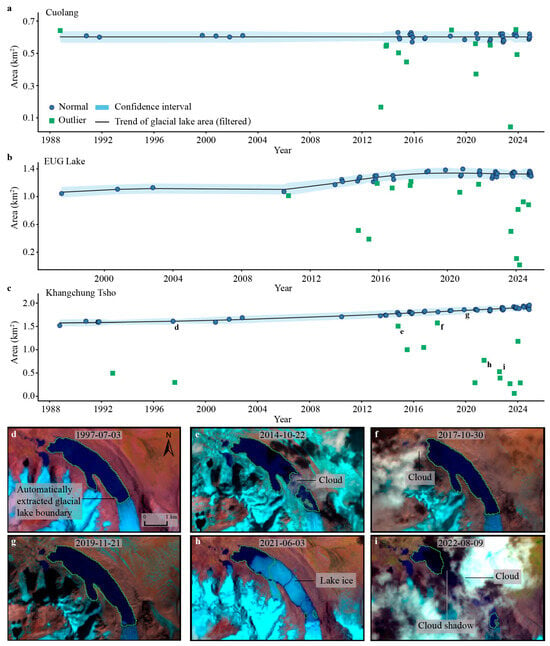
Figure 4. Examples of glacial lake anomaly detection and typical anomaly images. (a–c) Time series showing changes in the areas of the Cuolang, EUG, and Khangchung Tsho glacial lakes from 1988 to 2024, with anomalies highlighted. (d) Clear satellite image of Khangchung Tsho taken in July 1997. (e) Anomaly map from October 2014 highlighting lake ice on the surface of Khangchung Tsho. (f) October 2017 anomaly image affected by clouds. (g) Clear image of Khangchung Tsho from November 2019. (h) June 2021 anomaly image indicating lake ice, affected by anomalies. (i) August 2022 anomaly image obscured by clouds.

For EUG Lake (Figure 4b), the detection precision was 0.97. This method effectively eliminated anomalies caused by cloud interference after 2013, including those in 2014, 2016, 2020, 2023, and 2024, giving a more objective view of the long-term changes in the glacial lake area.

The Khangchung Tsho identified 14 anomaly points, of which 5 were caused by lake surface ice and 9 by cloud interference (Figure 4c). Examples include data from October 2014 (Figure 4e), October 2017 (Figure 4f), June 2021 (Figure 4h), and August 2022 (Figure 4i). After removing anomalies from 1989 to 2024, the average area was 1.57 km², showing a slight increase. This also affirms the accuracy of boundary extraction under cloud-free conditions, as demonstrated in July 1997 (Figure 4d) and November 2019 (Figure 4g).

The validation results for South Lhonak Lake (Figure 5a) demonstrate that the developed algorithm has strong generalization capabilities. Of 58 observation samples, 16 anomalies were correctly detected, achieving a Precision of 92% and an F1-score of 0.93. Once anomalies were removed, the data showed a steady increase from 1989 to 2024, with the lake area decreasing significantly to 1.4 km² after the 2023 outburst. The anomaly detection efficiently identified issues caused by cloud cover (Figure 5b,e), cloud shadows (Figure 5f), and ice formation on the lake surface (Figure 5c), enabling the construction of a high-quality, long-term dataset on glacial lake variations. These results validate the algorithm’s robustness in complex settings and offer dependable technical support for monitoring glacial lake dynamics.

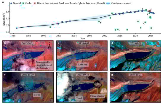
Figure 5. Anomaly detection at South Lhonak Lake and examples of typical anomaly images. (a) South Lhonak Lake area time series (1989–2024) showing anomalies, with an overall rise followed by a sharp drop after the 2023 outburst. (b) Cloud-covered anomaly image over the lake. (c) An anomaly image displaying ice formation on the lake’s surface. (d) Clear reference image of South Lhonak Lake under optimal conditions. (e) Cloud-affected anomaly image. (f) Cloud shadow impact on the lake anomaly image. (g) Accurate boundary delineation of the lake in 2023.

4.3. Comparison of Accuracy Among Different Models

To evaluate the performance of the EE-GP algorithm, we compared it with traditional methods. For a fair comparison, the baseline models were configured as follows: the Hampel filter used a fixed window size of 5 and a threshold of 3 median absolute deviations, representing a standard robust outlier-detection configuration. The ARIMA model parameters were customized for each lake’s time series: stationarity was verified by identifying the differencing order ‘d’ using the Augmented Dickey–Fuller test, followed by a grid search over autoregressive (‘p’) and moving average (‘q’) orders (ranging from 0 to 3) to find the model with the lowest AIC. This approach ensures that each baseline model is implemented in its standard or best-tuned form for time-series analysis.

Our research introduces a novel method for identifying glacial lake anomalies, achieving significant performance improvements. It reaches an F1-score of over 0.95, surpassing traditional approaches by 3–10% (Table 6). The algorithm effectively balances precision and recall. While the Hampel method attains a recall of 1.00, its precision drops to 0.87, indicating over-detection; the ARIMA model also exhibits lower precision. These results highlight the limitations of existing models and showcase the innovative research underpinning this approach.

Table 6. Comparison of the accuracy of the EF-GP algorithm with two traditional methods, Hampel and ARIMA.

Glacial Lake Name	Model	Precision	Recall	F1-Score	95% CI (F1-Score)
Cuolang	EF-GP	1.00	0.92	0.95	(0.9062, 1.0000)
	Hampel	0.88	1.00	0.94	(0.8767, 0.9880)
	ARIMA	0.86	1.00	0.93	(0.7907, 0.9375)
EUG Lake	EF-GP	0.97	0.95	0.96	(0.9231, 1.0000)
	Hampel	0.82	1.00	0.90	(0.8367, 0.9600)
	ARIMA	0.83	0.96	0.87	(0.8172, 0.9505)
Khangchung Tsho	EF-GP	0.98	1.00	0.99	(0.9684, 1.0000)
	Hampel	0.98	1.00	0.99	(0.9684, 1.0000)
	ARIMA	0.91	0.98	0.94	(0.8932, 0.9818)
South Lhonak Lake	EF-GP	0.92	0.94	0.93	(0.8750, 0.9867)
	Hampel	0.80	1.00	0.89	(0.8089, 0.9474)
	ARIMA	0.79	0.97	0.87	(0.7907, 0.9375)

Note: The 95% confidence intervals (95% CI) were determined using the bootstrap method with 1000 replicates to evaluate the stability of the F1-score estimates.

Analysis shows that EF-GP improves the stability of glacial lake time series after removing anomalies (Figure 6). In Cuolang Lake, EF-GP detects early anomalies that traditional methods overlook. For EUG Lake, it filters interference more effectively and clearly displays the lake’s continued growth since 1998, outperforming conventional techniques. At Khangchung Tsho, both EF-GP and Hampel successfully identify anomalies. During the outburst at South Lhonak Lake, EF-GP tracked fluctuations more accurately than traditional methods. Overall, EF-GP demonstrates to be a dependable and effective tool for detecting anomalies in glacial lakes.

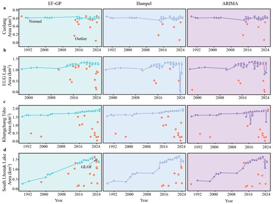
Figure 6. A comparative assessment of anomaly detection algorithms applied to four glacial lakes: (a) Cuolang Lake, (b) EUG Lake, (c) Khangchung Tsho, and (d) South Lhonak Lake. The EF-GP approach demonstrates improved time series stability after removing anomalies, with better early detection in Cuolang, more effective interference filtering in EUG, and more accurate monitoring of lake fluctuations during outburst events in South Lhonak.

5. Discussion

Our study presents a Gaussian process method for identifying anomalies associated with changes in glacial lake areas, surpassing traditional time-series analysis methods. Methods like the Hampel filter and ARIMA have limitations: the Hampel filter can generate false alarms due to seasonal variations [34], potentially leading to the misinterpretation of natural lake growth as glacier retreat; similarly, ARIMA, which assumes linearity [57,58], struggles to identify sudden nonlinear events such as GLOFs. The EF-GP algorithm introduces three improvements: (1) using Gaussian processes to model lake data without predefined functions; (2) employing double-validation based on lake evolution to capture GLOF features; (3) and iterative optimization to improve precision by detecting anomalies and refining the model. Results show EF-GP effectively detects anomalies aligned with lake patterns.

While the EF-GP algorithm’s advantages are evident, its application is mainly confined to moraine-dammed lakes, which typically experience single, isolated outburst events. It is less effective for ice-dammed glacial lakes [57], which undergo frequent seasonal filling and drainage cycles, as physical constraints—like the assumption that lakes shrink over a long period after an event—may not hold. Future research should aim to develop methods for anomaly detection in ice-dammed lakes, particularly those with repeated, high-frequency outbursts.

These issues mainly arise from: (1) the Gaussian process’s limited ability to capture high-frequency, sudden changes accurately [59]; (2) the restricted flexibility of optimized parameters when faced with abrupt, intense shifts; and (3) the missing data caused by clouds and snow, which cause gaps in remote sensing time series and reduce accuracy [60].

Another methodological limitation arises from the use of stationary kernels in our Gaussian Process model. When working with sparse data from early periods, their inherent smoothing can underestimate or hide isolated anomalies in the historical record. This study included images with less than 30% cloud cover, but there were notable data gaps from 1988 to 2016, primarily caused by high cloud cover (Figure 7a). For example, the August 1997 image of Longbasaba Lake was affected by cloud shadows (Figure 7b), resulting in an underestimated lake area. This anomaly was overlooked because the overall increasing trend of lake size masked it. The adoption of high-spatiotemporal-resolution satellite systems, such as Sentinel-2, is expected to produce more continuous and complete time-series data on glacial lakes.

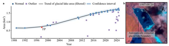
Figure 7. A case study of anomaly detection at Longbasaba Lake. (a) Time series for the Longbasaba Lake area (1989–2024), showing detected anomalies (Outlier) and misclassified observations (False positive, FP). (b) An example of a lake boundary anomaly caused by cloud and cloud shadow.

Despite certain limitations, EF-GP shows considerable promise for advancing research on glacial lakes and assessing risks. It provides a systematic approach to detecting GLOF events that might have previously gone unrecorded or poorly documented. This facilitates the creation of more complete GLOF records, particularly in remote mountain regions with sparse direct observations [61]. Moreover, EF-GP enhances data quality control for automatically gathered glacial lake datasets. Although it does not directly improve pixel-level segmentation accuracy, it acts as a temporal filter, removing false fluctuations caused by clouds, snow, or terrain shadows, thereby enhancing the reliability of long-term data. The algorithm is highly adaptable to various regions. Thanks to the extensive history and broad coverage of remote sensing imagery, such as Landsat [62], EF-GP can be applied to glacial lake monitoring elsewhere, provided a sufficient time series of lake-area data is available. It performs best with lakes that show relatively stable area changes and have few documented outburst events.

Future improvements include: (1) using non-stationary kernel functions to better model and detect sudden changes [63]; (2) adopting trend-sensitive weighting methods to improve detection of small lake area reductions [64]; and (3) combining multiple remote sensing sources, such as SAR, to enhance glacial lake monitoring over time [65].

6. Conclusions

This study presents a Gaussian process-based anomaly detection method that utilizes features of glacial lake evolution. By combining non-parametric models with physical constraints, it establishes a unified criterion that significantly improves the accuracy of detecting anomalies in glacial lakes. Testing on typical Himalayan glacial lakes shows that the method achieves an average F1-score of 95%, effectively addressing issues caused by cloud cover and terrain shadowing.

Our algorithm effectively detects anomalies, providing reliable support for developing a high-quality, long-term dataset on glacial lakes using satellite remote sensing. This greatly enhances the accuracy of monitoring changes over time. As a result, it has the potential to scale for real-time water volume monitoring and remote sensing of water level fluctuations. Future work will focus on improving multi-source remote sensing data fusion techniques to address challenges in heavily clouded areas and to enhance their application for ice-dammed lakes, ultimately integrating them into monitoring and early warning systems for high-risk glacial lakes.

References

- Tang, Q.; Zhang, G.; Yao, T.; Wieland, M.; Liu, L.; Kaushik, S. Automatic extraction of glacial lakes from Landsat imagery using deep learning across the Third Pole region. Remote Sens. Environ. 2024, 315, 114413. [Google Scholar] [CrossRef]
- Mir, R.A.; Jain, S.K.; Lohani, A.K.; Saraf, A.K. Glacier recession and glacial lake outburst flood studies in Zanskar basin, western Himalaya. J. Hydrol. 2018, 564, 376–396. [Google Scholar] [CrossRef]
- Shrestha, F.; Steiner, J.F.; Shrestha, R.; Dhungel, Y.; Joshi, S.P.; Inglis, S.; Ashraf, A.; Wali, S.; Walizada, K.M.; Zhang, T. A comprehensive and version-controlled database of glacial lake outburst floods in High Mountain Asia. Earth Syst. Sci. Data 2023, 15, 3941–3961. [Google Scholar] [CrossRef]
- Nie, Y.; Sheng, Y.; Liu, Q.; Liu, L.; Liu, S.; Zhang, Y.; Song, C. A regional-scale assessment of Himalayan glacial lake changes using satellite observations from 1990 to 2015. Remote Sens. Environ. 2017, 189, 1–13. [Google Scholar] [CrossRef]
- Ke, L.; Ding, X.; Ning, Y.; Liao, Y.; Song, C. Annual trajectory of global glacial lake variations and the interactions with glacier mass balance during 2013–2022. Catena 2024, 245, 108280. [Google Scholar] [CrossRef]
- Chen, M.; Chen, Y.; Fang, G.; Zheng, G.; Li, Z.; Li, Y.; Zhu, Z. Risk assessment of glacial lake outburst flood in the Central Asian Tienshan Mountains. npj Clim. Atmos. Sci. 2024, 7, 209. [Google Scholar] [CrossRef]
- Song, C.; Huang, B.; Richards, K.; Ke, L.; Hien Phan, V. Accelerated lake expansion on the Tibetan Plateau in the 2000s: Induced by glacial melting or other processes? Water Resour. Res. 2014, 50, 3170–3186. [Google Scholar] [CrossRef]
- Nie, Y.; Pritchard, H.D.; Liu, Q.; Hennig, T.; Wang, W.; Wang, X.; Liu, S.; Nepal, S.; Samyn, D.; Hewitt, K.; et al. Glacial change and hydrological implications in the Himalaya and Karakoram. Nat. Rev. Earth Environ. 2021, 2, 91–106. [Google Scholar] [CrossRef]
- Liu, W.; Carling, P.A.; Hu, K.; Wang, H.; Zhou, Z.; Zhou, L.; Liu, D.; Lai, Z.; Zhang, X. Outburst floods in China: A review. Earth-Sci. Rev. 2019, 197, 102895. [Google Scholar] [CrossRef]
- Wang, W.; Nie, Y.; Zhang, H.; Wang, J.; Deng, Q.; Liu, L.; Liu, F.; Zhang, S.; Lyu, Q.; Zhang, L. A generic framework for glacial lake outburst flood investigation: A case study of Zalai Tsho, Southeast Tibet. Catena 2024, 234, 107614. [Google Scholar] [CrossRef]
- Yan, W.; Liu, J.; Zhang, M.; Hu, L.; Chen, J. Outburst flood forecasting by monitoring glacier-dammed lake using satellite images of Karakoram Mountains, China. Quat. Int. 2017, 453, 24–36. [Google Scholar] [CrossRef]
- Veh, G.; Korup, O.; von Specht, S.; Roessner, S.; Walz, A. Unchanged frequency of moraine-dammed glacial lake outburst floods in the Himalaya. Nat. Clim. Change 2019, 9, 379–383. [Google Scholar] [CrossRef]
- Prakash, C.; Nagarajan, R. Glacial Lake Inventory and Evolution in Northwestern Indian Himalaya. IEEE J. Sel. Top. Appl. Earth Observ. Remote Sens. 2017, 10, 5284–5294. [Google Scholar] [CrossRef]
- Jiang, D.; Li, S.; Hajnsek, I.; Siddique, M.A.; Hong, W.; Wu, Y. Glacial lake mapping using remote sensing Geo-Foundation Model. Int. J. Appl. Earth Obs. Geoinf. 2025, 136, 104371. [Google Scholar] [CrossRef]
- Manu, T.; Yuchang, J.; Emmanuel, B.; Konrad, S. Learning a Joint Embedding of Multiple Satellite Sensors: A Case Study for Lake Ice Monitoring. IEEE Trans. Geosci. Remote Sens. 2022, 60, 4306315. [Google Scholar] [CrossRef]
- Medeu, A.R.; Popov, N.V.; Blagovechshenskiy, V.P.; Askarova, M.A.; Medeu, A.A.; Ranova, S.U.; Kamalbekova, A.; Bolch, T. Moraine-dammed glacial lakes and threat of glacial debris flows in South-East Kazakhstan. Earth-Sci. Rev. 2022, 229, 103999. [Google Scholar] [CrossRef]
- Williamson, A.G.; Banwell, A.F.; Willis, I.C.; Arnold, N.S. Dual-satellite (Sentinel-2 and Landsat 8) remote sensing of supraglacial lakes in Greenland. Cryosphere 2018, 12, 3045–3065. [Google Scholar] [CrossRef]
- Lesi, M.; Nie, Y.; Shugar, D.H.; Wang, J.; Deng, Q.; Chen, H.; Fan, J. Landsat- and Sentinel-derived glacial lake dataset in the China–Pakistan Economic Corridor from 1990 to 2020. Earth Syst. Sci. Data 2022, 14, 5489–5512. [Google Scholar] [CrossRef]
- Wang, J.; Chen, F.; Zhang, M.; Yu, B. ACFNet: A Feature Fusion Network for Glacial Lake Extraction Based on Optical and Synthetic Aperture Radar Images. Remote Sens. 2021, 13, 5091. [Google Scholar] [CrossRef]
- Wu, R.; Liu, G.; Zhang, R.; Wang, X.; Li, Y.; Zhang, B.; Cai, J.; Xiang, W. A Deep Learning Method for Mapping Glacial Lakes from the Combined Use of Synthetic-Aperture Radar and Optical Satellite Images. Remote Sens. 2020, 12, 4020. [Google Scholar] [CrossRef]
- Cheng, X.; Shangguan, D.; Yang, C.; Li, W.; Zhou, Z.; Liu, X.; Li, D.; Zhang, X.; Ding, H.; Liu, Z.; et al. Temporal and spatial changes of glacial lakes in the central Himalayas and their response to climate change based on multi-source remote sensing data. Glob. Planet. Change 2025, 245, 104675. [Google Scholar] [CrossRef]
- Xu, X.; Liu, L.; Huang, L.; Hu, Y. Combined use of multi-source satellite imagery and deep learning for automated mapping of glacial lakes in the Bhutan Himalaya. Sci. Remote Sens. 2024, 10, 100157. [Google Scholar] [CrossRef]
- Allen, S.K.; Rastner, P.; Arora, M.; Huggel, C.; Stoffel, M. Lake outburst and debris flow disaster at Kedarnath, June 2013: Hydrometeorological triggering and topographic predisposition. Landslides 2016, 13, 1479–1491. [Google Scholar] [CrossRef]
- Veh, G.; Korup, O.; Roessner, S.; Walz, A. Detecting Himalayan glacial lake outburst floods from Landsat time series. Remote Sens. Environ. 2018, 207, 84–97. [Google Scholar] [CrossRef]
- Song, C.; Fan, C.; Ma, J.; Zhan, P.; Deng, X. A spatially constrained remote sensing-based inventory of glacial lakes worldwide. Sci. Data 2025, 12, 464. [Google Scholar] [CrossRef]
- Shi, H.; Guo, J.; Deng, Y.; Qin, Z. Machine learning-based anomaly detection of groundwater microdynamics: Case study of Chengdu, China. Sci. Rep. 2023, 13, 14718. [Google Scholar] [CrossRef]
- Goldstein, M.; Uchida, S. A Comparative Evaluation of Unsupervised Anomaly Detection Algorithms for Multivariate Data. PLoS ONE 2016, 11, e152173. [Google Scholar] [CrossRef]
- Filho, J.A.P.; Neves, C.F.; Lopes, W.T.A.; Carvalho, J.C. Anomaly detection in hydrological network time series via multiresolution analysis. J. Hydrol. 2024, 640, 131667. [Google Scholar] [CrossRef]
- Hampel, F.R. The Influence Curve and its Role in Robust Estimation. J. Am. Stat. Assoc. 1974, 69, 383–393. [Google Scholar] [CrossRef]
- Jeong, J.; Park, E.; Han, W.S.; Kim, K.; Choung, S.; Chung, I.M. Identifying outliers of non-Gaussian groundwater state data based on ensemble estimation for long-term trends. J. Hydrol. 2017, 548, 135–144. [Google Scholar] [CrossRef]
- Chang, L.; Cheng, L.; Zhang, L.; Han, D.; Zhang, J.; Liu, P. Remote sensing-based high-resolution reservoir drought index for identifying the occurrence and propagation of hydrological droughts in a large river basin. Remote Sens. Environ. 2025, 328, 114859. [Google Scholar] [CrossRef]
- Dømgaard, M.; Kjeldsen, K.; How, P.; Bjørk, A. Altimetry-based ice-marginal lake water level changes in Greenland. Commun. Earth Environ. 2024, 5, 365. [Google Scholar] [CrossRef]
- Berendrecht, W.; van Vliet, M.; Griffioen, J. Combining statistical methods for detecting potential outliers in groundwater quality time series. Environ. Monit. Assess. 2022, 195, 85. [Google Scholar] [CrossRef] [PubMed]
- Yan, J.; Tao, T. Unsupervised anomaly detection in hourly water demand data using an asymmetric encoder–decoder model. J. Hydrol. 2022, 613, 128389. [Google Scholar] [CrossRef]
- Mishra, A.; Sriharsha, R.; Zhong, S. OnlineSTL: Scaling time series decomposition by 100x. Proc. VLDB Endow. 2022, 15, 1417–1425. [Google Scholar] [CrossRef]
- Leigh, C.; Alsibai, O.; Hyndman, R.J.; Kandanaarachchi, S.; King, O.C.; McGree, J.M.; Neelamraju, C.; Strauss, J.; Talagala, P.D.; Turner, R.D.R.; et al. A framework for automated anomaly detection in high frequency water-quality data from in situ sensors. Sci. Total Environ. 2019, 664, 885–898. [Google Scholar] [CrossRef]
- Feng, Y.; Liu, Z.; Liu, Q.; Wang, Z. Hydrologic Time Series Anomaly Detection Based on Flink. Math. Probl. Eng. 2020, 2020, 3187697. [Google Scholar] [CrossRef]
- Breunig, M.M.; Kriegel, H.; Ng, R.T.; Sander, J. LOF: Identifying density-based local outliers. In Proceedings of the 2000 ACM SIGMOD International Conference on Management of Data, Dallas, TX, USA, 15–18 May 2000; Association for Computing Machinery: New York, NY, USA, 2000; pp. 93–104. [Google Scholar]
- Hochreiter, S.; Schmidhuber, J. Long short-term memory. Neural Comput. 1997, 9, 1735–1780. [Google Scholar] [CrossRef]
- Mokua, N.; Maina, C.W.; Kiragu, H. Anomaly detection for raw water quality—A comparative analysis of the local outlier factor algorithm and the random forest algorithms. Int. J. Comput. Appl. 2021, 174, 47–54. [Google Scholar] [CrossRef]
- Arathy Nair, G.R.; Adarsh, S. Anomaly Detection of Streamflow Time Series Using LSTM Autoencoder. AIJR Proc. 2023, 112–119. [Google Scholar] [CrossRef]
- Choi, K.; Yi, J.; Park, C.; Yoon, S. Deep Learning for Anomaly Detection in Time-Series Data: Review, Analysis, and Guidelines. IEEE Access 2021, 9, 120043–120065. [Google Scholar] [CrossRef]
- De la Fuente, L.A.; Ehsani, M.R.; Gupta, H.V.; Condon, L.E. Toward interpretable LSTM-based modeling of hydrological systems. Hydrol. Earth Syst. Sci. 2024, 28, 945–971. [Google Scholar] [CrossRef]
- Nie, Y.; Liu, Q.; Wang, J.; Zhang, Y.; Sheng, Y.; Liu, S. An inventory of historical glacial lake outburst floods in the Himalayas based on remote sensing observations and geomorphological analysis. Geomorphology 2018, 308, 91–106. [Google Scholar] [CrossRef]
- Yu, Y.; Li, B.; Li, Y.; Jiang, W. Retrospective Analysis of Glacial Lake Outburst Flood (GLOF) Using AI Earth InSAR and Optical Images: A Case Study of South Lhonak Lake, Sikkim. Remote Sens. 2024, 16, 2307. [Google Scholar] [CrossRef]
- Jiang, D.; Li, X.; Zhang, K.; Marinsek, S.; Hong, W.; Wu, Y. Automatic Supraglacial Lake Extraction in Greenland Using Sentinel-1 SAR Images and Attention-Based U-Net. Remote Sens. 2022, 14, 4998. [Google Scholar] [CrossRef]
- Sharma, A.; Prakash, C.; Thakur, D. Glacier lakes detection utilizing remote sensing integration with satellite imagery and advanced deep learning method. Appl. Geomat. 2024, 16, 829–850. [Google Scholar] [CrossRef]
- Zhang, H.; Nie, Y.; Liu, L.; Han, L.; Lyu, Q.; Wang, W. An advanced deep learning framework for mapping glacial lakes and its application in the Hindu Kush-Karakoram-Himalaya region. J. Hydrol. 2026, 664, 134507. [Google Scholar] [CrossRef]
- Wang, J.; Sheng, Y.; Tong, T.S.D. Monitoring decadal lake dynamics across the Yangtze Basin downstream of Three Gorges Dam. Remote Sens. Environ. 2014, 152, 251–269. [Google Scholar] [CrossRef]
- Rasmussen, C.E. Gaussian processes in machine learning. In Summer School on Machine Learning; Springer: Berlin/Heidelberg, Germany, 2003; pp. 63–71. [Google Scholar]
- Deisenroth, M.P.; Turner, R.D.; Huber, M.F.; Hanebeck, U.D.; Rasmussen, C.E. Robust Filtering and Smoothing with Gaussian Processes. IEEE Trans. Autom. Control. 2012, 57, 1865–1871. [Google Scholar] [CrossRef]
- Oh, G.L.; Austin, P.H. Quantifying the oscillatory evolution of simulated boundary-layer cloud fields using Gaussian process regression. Geosci. Model Dev. 2025, 18, 3921–3940. [Google Scholar] [CrossRef]
- Pascual-Venteo, A.B.; Garcia, J.L.; Berger, K.; Estévez, J.; Vicent, J.; Pérez-Suay, A.; Van Wittenberghe, S.; Verrelst, J. Gaussian Process Regression Hybrid Models for the Top-of-Atmosphere Retrieval of Vegetation Traits Applied to PRISMA and EnMAP Imagery. Remote Sens. 2024, 16, 1211. [Google Scholar] [CrossRef]
- Susiluoto, J.; Spantini, A.; Haario, H.; Härkönen, T.; Marzouk, Y. Efficient multi-scale Gaussian process regression for massive remote sensing data with satGP v0.1.2. Geosci. Model Dev. 2020, 13, 3439–3463. [Google Scholar] [CrossRef]
- Mukangango, J.; Muyskens, A.; Priest, B.W. A robust approach to Gaussian process implementation. Adv. Stat. Clim. Meteorol. Oceanogr. 2024, 10, 143–158. [Google Scholar] [CrossRef]
- Hanshaw, M.N.; Bookhagen, B. Glacial areas, lake areas, and snow lines from 1975 to 2012: Status of the Cordillera Vilcanota, including the Quelccaya Ice Cap, northern central Andes, Peru. Cryosphere 2014, 8, 359–376. [Google Scholar] [CrossRef]
- Pehlivan, H. A novel outlier detection method based on Bayesian change point analysis and Hampel identifier for GNSS coordinate time series. EURASIP J. Adv. Signal Process. 2024, 2024, 44. [Google Scholar] [CrossRef]
- Zhang, G.P. Time series forecasting using a hybrid ARIMA and neural network model. Neurocomputing 2003, 50, 159–175. [Google Scholar] [CrossRef]
- Fox, E.B.; Dunson, D.B. Multiresolution Gaussian processes. In Proceedings of the 26th International Conference on Neural Information Processing Systems, Lake Tahoe, NV, USA, 3–6 December 2012; Curran Associates Inc.: Red Hook, NY, USA, 2012; Volume 1, pp. 737–745. [Google Scholar]
- Siabi, N.; Sanaeinejad, S.H.; Ghahraman, B. Effective method for filling gaps in time series of environmental remote sensing data: An example on evapotranspiration and land surface temperature images. Comput. Electron. Agric. 2022, 193, 106619. [Google Scholar] [CrossRef]
- Emmer, A.; Wood, J.L.; Cook, S.J.; Harrison, S.; Wilson, R.; Diaz-Moreno, A.; Reynolds, J.M.; Torres, J.C.; Yarleque, C.; Mergili, M.; et al. 160 glacial lake outburst floods (GLOFs) across the Tropical Andes since the Little Ice Age. Glob. Planet. Change 2022, 208, 103722. [Google Scholar] [CrossRef]
- Viana, C.M.; Girão, I.; Rocha, J. Long-Term Satellite Image Time-Series for Land Use/Land Cover Change Detection Using Refined Open Source Data in a Rural Region. Remote Sens. 2019, 11, 1104. [Google Scholar] [CrossRef]
- Paun, I.; Husmeier, D.; Torney, C.J. Stochastic variational inference for scalable non-stationary Gaussian process regression. Stat. Comput. 2023, 33, 44. [Google Scholar] [CrossRef]
- Zeng-Guang, Z.; Ping, T. Improving time series anomaly detection based on exponentially weighted moving average (EWMA) of season-trend model residuals. In Proceedings of the 2016 IEEE International Geoscience and Remote Sensing Symposium (IGARSS), Beijing, China, 10–15 July 2016; pp. 3414–3417. [Google Scholar]
- Pipia, L.; Muñoz-Marí, J.; Amin, E.; Belda, S.; Camps-Valls, G.; Verrelst, J. Fusing optical and SAR time series for LAI gap filling with multioutput Gaussian processes. Remote Sens. Environ. 2019, 235, 111452. [Google Scholar] [CrossRef] [PubMed]
Disclaimer/Publisher’s Note: The statements, opinions and data contained in all publications are solely those of the individual author(s) and contributor(s) and not of MDPI and/or the editor(s). MDPI and/or the editor(s) disclaim responsibility for any injury to people or property resulting from any ideas, methods, instructions or products referred to in the content. |
© 2025 by the authors. Licensee MDPI, Basel, Switzerland. This article is an open access article distributed under the terms and conditions of the Creative Commons Attribution (CC BY) license.