Highlights
What are the main findings?
- A new method refines error prediction, reducing the uncertainty in a subglacial topography for 56% of a widely used Greenland Ice Sheet (GrIS) bed topography dataset.
- The adjusted Greenland bed dataset suggested a 7 mm higher sea-level equivalent ice volume and a 29% increase in area grounded > 200 m below sea level.
What are the implications of the main findings?
- Refined error estimation for ice sheet bed topography datasets derived by kriging.
- A 29% increase in the area of the interior GrIS bed was estimated to be >200 m below sea level, indicating that a larger area of the ice sheet is potentially more susceptible than previously estimated to submarine melting in the long term.
Abstract
Subglacial topography is a critical boundary condition for ice sheet models projecting past and future ice sheet–climate interactions. Contemporary ice-sheet-wide bed topography datasets are partially derived using mass conservation, but approximately 75% of the most widely used Greenland Ice Sheet (GrIS) dataset is based on simple interpolation of airborne radio-echo sounding (RES) measurements, such as kriging or streamline diffusion. Due to limited independent validation data, the errors and biases in this approach are poorly understood, creating largely unknown uncertainties in subglacial topography. Here, we interpolated synthetic RES observations of bed topography over ice-free areas with a known topography at a 5 m spatial resolution and quantify discrepancies. We found that the absolute error in kriged bed topography increases with distance from the input data, though at a reduced rate than previously estimated. The difference between an interpolated elevation estimate and the local mean elevation is a strong predictor of real bed errors (R2 = 0.72), with further improvement as input observation sparsity increases (R2 > 0.82). We propose a method to quantify and reduce uncertainty in kriged bed topography in sparsely surveyed regions, reducing uncertainty for at least 56% of the kriged interior at a 99% confidence interval. Our results suggest that subglacial depth is on average 5 m deeper than previous estimates, though individual areas may be shallower or deeper (σ = 41 m). Consequently, the area grounded below sea level is likely underestimated by 2%, increasing to 29% for regions deeper than 200 m. These findings have potential implications for the future stability of the GrIS under climate change.
1. Introduction
Quantification of ice thickness and subglacial topography over an entire ice sheet is essential for understanding how it is likely to change with the climate [1]. Ice-sheet-wide ice thickness estimates are used to determine the volume and, subsequently, mass of an ice sheet. From this, a measure of the total potential contribution to sea-level rise contained by the ice sheet can be derived [2]. Moreover, quantification of subglacial topography is essential as it is a first-order control on the rate at which the ice sheet responds to perturbations such as climate change [3]. Hence, an accurate description of the bed topography and ice thickness is of paramount importance for numerical modelling efforts to estimate contributions from the ice sheets to global sea-level rise. Ice thickness is typically measured using airborne radio-echo sounding (RES) techniques. Subsequently, subglacial topography is derived by subtracting the thickness measurement from the surface elevation [4], which is typically measured simultaneously using an airborne laser altimeter. While RES surveys have been conducted for decades and cover hundreds of thousands of kilometres of ice [5], due to the scale of ice sheets, ice caps, and glaciers, the overall measurement coverage is sparse [6]. For example, the mean flight-line spacing across the Greenland Ice Sheet (GrIS) interior is ~18 ± 24 km. In order to quantify ice thickness and bed elevation in areas between measurements, spatial interpolation is required (e.g., [7]). Various methods have been implemented to achieve this, all of which have associated uncertainties (e.g., [7,8,9,10,11]). As current projections of sea-level change are increasingly using ice dynamical models, robust quantification of and reduction in these uncertainties is essential for producing reliable projections [12].
Ice thickness has been surveyed for over 5 decades across the continental ice sheets (Greenland: [6]; Antarctica: [13]). From these surveys, it has been possible to map ice thickness and, subsequently, bed topography across the GrIS [1,7,9] and Antarctic Ice Sheets [14,15,16,17] through interpolation and modelling. The most recent efforts have achieved this using mass conservation techniques close to the ice margins, where RES instruments typically perform less well due to extensive crevassing, which scatters the radar signal [9,17,18]. These datasets are becoming widely used for studies on ice sheet bed topography. Mass conservation combines observations of surface velocity with measurements of ice thickness to infer ice sheet bed topography in regions of fast flow (typically > 50 ma−1) [19]. However, ice flow in many marginal areas of the GrIS has been observed to be highly variable over seasonal and interannual timescales [20,21]; as such, velocity values selected to generate the bed may not be entirely representative of the longer-term ice flow, which may lead to the introduction of errors. Furthermore, in areas of slower ice flow (<50 ma−1), other interpolation approaches are required, as the mass conservation approach requires a minimum observed ice flow [17]. For instance, in Bedmachine Antarctica, streamline diffusion is used as an alternative, which utilises the direction of ice flow to interpolate ice thickness between flight-lines anisotropically, resulting in a “realistic” bed profile consistent with the mass conservation-derived regions [17].
Kriging is a geostatistical interpolator that has traditionally been the chosen method for deriving the wide-scale bed topography of ice masses [1,7,16,22], because it is optimal for irregularly sampled input measurements and provides a best estimate for values in under-sampled regions [23]. However, known limitations of the method are that it tends to smooth a landscape toward a mean value and that it cannot accurately reproduce channel-like subglacial landforms [8,24]. This leads to the introduction of artefacts in derived subglacial topography datasets, which occur at scales that ice dynamics are sensitive to (~1 km) [17,25]. It also leads to the underestimation of bed elevation in upland areas and the overestimation of elevations in lowlands, thereby consistently underestimating subglacial relief [24,25]. Smoothing topography in such a way has implications for the overall roughness of the bed in the output data. Furthermore, this obfuscates potentially important bedforms or areas of local roughness, which potentially exert a strong influence on ice dynamics [25], resulting in erroneous bed inputs to ice sheet models, which subsequently may not be able to accurately replicate observed flow dynamics. This is particularly important for modelling grounding line retreat, where the presence of high-relief basal topographic features can limit retreat. Where these features are smoothed out in bed interpolations, predicted retreat will tend to be faster.
However, ordinary kriging remains a widely used and expedient method of interpolating subglacial topography. Despite these well-known limitations, the quantification of uncertainties in the method is rarely constrained other than “built-in” simple inverse distance relationships with respect to the location of the input data [1]. Furthermore, various analytical outputs derived from bed topography often implement broad uncertainties in ice thickness (e.g., [26]), which carry through into important assessments of ice sheet mass balance and stability (e.g., [27]). Hence, a more reliable prediction of these errors could improve quantification of uncertainty in ice sheet model projections.
Ice sheet models used in ISMIP6, which contributes to CMIP6 projections of sea-level change, use a variety of bed topography datasets as inputs [12,17]. As ordinary kriging is employed for much of the preceding subglacial topography data [1,16], and for significant portions of newer data [9], it is important that uncertainties associated with these datasets are well constrained in order to provide reliable uncertainties in the contribution of the ice sheets to sea-level rise. This becomes especially critical where uncertainty quantification for projections of future sea-level rise is directly based on error estimates of the input data. Therefore, assessing the uncertainty in kriged bed topography more precisely and developing more reliable estimates of ice thickness and bed elevation errors would be beneficial to our comprehension of ice sheets and future projections of sea-level change [12,28].
Validation of RES-derived ice thickness datasets is challenging as it either requires physically accessing the ice sheet bed through 1000s of metres of ice, or an in situ geophysical survey using radar and seismic approaches. Either way, it is logistically challenging and costly, so development of reliable estimates of uncertainty is critical in the absence of ground-truthing. Using high-resolution (two metres) Arctic DEM digital elevation data for ice-free proglacial areas of Greenland [29], recent work [30] has shown it is possible to investigate the uncertainties and biases of interpolation techniques by simulating RES surveys over DEMs of known topography, interpolating the resultant synthetic measurements, and comparing the output interpolation with the input DEM. This study aims to better understand the uncertainties arising when interpolating RES data by developing a method for estimating errors in subglacial topography using proximal and geomorphologically similar ice-free topography. From this, previous datasets of kriged bed topography may be used with higher confidence, and new bed topography may be generated with accompanying maps of uncertainty. Hence, this reduces the uncertainty in 3D bed topography datasets generated by kriging, beyond methods for 2D and RES input measurements only [30]. Here, we focus on the GrIS as a case study, note the implications of our results for GrIS, and discuss the implications for other ice masses and bed topography datasets derived by kriging.
2. Materials and Methods
2.1. Study Locations and Datasets
Digital elevation model (DEM) tiles of four regions of glaciated terrain were acquired from the ArcticDEM and aggregated to five-metre cell sizes for computational efficiency [29]. Three regions, Inglefield Land, Kangerlussuaq, and Peary Land, were selected from the margin proximal proglacial areas around the GrIS (Figure 1). These regions were selected as landscape ‘archetypes’; they comprise different scales of relief and are likely similar in geometry to their respective adjoining regions of subglacial topography [31]. Inglefield Land is characterised by low-relief, minimally eroded terrain, likely preserved beneath cold-based ice, representative of smooth beds in the GrIS interior [9]. Kangerlussuaq exhibits subdued relief and a really scoured topography, which is common beneath continental ice sheets [9,32]. Peary Land is dominated by fjords, troughs, and plateaus, representative of large portions of the northern and eastern GrIS bed [10]. While these regions capture a broad range of subglacial topographic conditions, they do not encompass all possible bed topography configurations or regions of pervasive marine influence. The availability of proglacial topography data is limited in Eastern and South-Eastern Greenland, as the region consists largely of marine-terminating outlet glaciers and submerged fjords. Correspondingly, limited elevation data are available, and bathymetric data in such areas are either unavailable or not of comparable resolution to the ArcticDEM and, therefore, insufficient for our analysis. Hence, landscape-type four was selected from a topographically similar area of the McKenzie Mountains in Canada, which was previously glaciated by the Cordilleran ice sheet ([33] and references within), and used as an East Greenland Analogue (EGA). Each study site covers an area of approximately 50 km by 50 km. Although the selected landscapes are presently ice-free and will have experienced some post-glacial modification, at the spatial scales relevant to this study, they are considered broadly representative of the underlying subglacial topography.
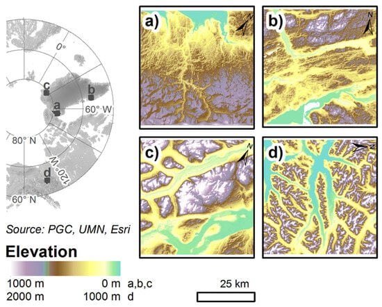
Figure 1.
Study sites: (a) Inglefield Land; (b) Kangerlussuaq; (c) Peary Land; and (d) EGA.
2.2. Synthetic RES Survey Data
To fully simulate the generation of subglacial topography from acquisition to interpolation, we generated synthetic RES surveys over the input DEMs. Synthetic RES surveys were simulated by implementing the geospatial RES simulation method outlined by [30]. We mimicked the various geometries of RES surveys conducted by Operation IceBridge over Greenland [34]. Accordingly, flight-lines were simulated for margin parallel (MP) and margin orthogonal (MO) orientations, as well as for gridded surveys. The flight-line density was variable across surveys (e.g., references within the “Data” section of [5]); therefore, we conducted synthetic surveys at 1, 5, 10, and 15 km spacings to represent the broad range of RES survey densities across the Greenland Ice Sheet [34]. Simulated picked elevations were sampled at a ~15 m spacing along-track. Negative bias resulting from off-nadir elevation differences was alleviated by applying a mean shift to the input data points [30]. As ice bottom errors resulting from the attenuation and scattering of the radar signal by various facets of the ice sheet environment were not parameterised, the uncertainty in the simulated measurements was equivalent to the uncertainty of the ArcticDEM (~1 m vertically and ~0.1 m horizontally; [29]).
2.3. Kriging
Due to its widespread use in geosciences and our overarching aim to simulate and quantify uncertainty in bed topography akin to previous and ongoing studies, we interpolated surfaces from our synthetic RES survey data using kriging [19]. Surfaces were interpolated for each study site for the three survey geometries (MP, MO, and grids) and the four line spacings (1, 5, 10, and 15 km). Ordinary kriging was conducted in ArcGIS 10.5.1 using the inbuilt geostatistical tools, following the method of [35]. A spherical model was used, and algorithm parameters were optimised using ArcMap’s inbuilt iterative cross-validation technique (Table S1).
2.4. Quality Assessment of Bed Topography Interpolations
Each realisation of interpolated bed topography was differenced from the source DEM for each study site. Spatially random sample points were generated across each study site, with a minimum spacing of 150 m, aligned with the gridded resolution of Bedmachine Greenland v3. For each 50 × 50 km spacing, approximately 20,000 points could be generated. Across all output surfaces, this totalled 1.5 million observations. At each point, the differences in elevation between the interpolations and the DEM were sampled. Differences in elevation of an interpolated point from the same location on the DEM are herein referred to as interpolation errors. The overall interpolation error was defined as the standard deviation of all the interpolation errors. The root mean square deviation along each input flight-line was calculated as a measure of bed roughness. This measure was also compared with the overall elevation error for the interpolated bed. Additionally, the Euclidean distance of each point from an input location was calculated for all survey geometries.
2.5. Uncertainty Reduction
To improve the estimates of the uncertainty in bed topography and, consequently, ice thickness, firstly, the interpolation error magnitude was compared with the distance from the input. This assessed the interpolation error as a function of distance from a direct measurement, as opposed to the widely used method of posing a prescribed exponential increase in interpolation uncertainty with distance, which is a by-product of kriging. Secondly, the difference in an interpolated elevation from the regional (50 km × 50 km neighbourhood) mean elevation of the interpolation, termed the difference from the mean elevation (DME), was compared with the interpolation error. This aimed to exploit the known limitation of kriging, where the output surface is smoothed towards the mean elevation of the inputs. Ordinary least squares regression was calculated for these variables to develop a function to be applied to the kriged bed topography. Where suitable, this function was applied to kriged regions of BedMachine Greenland v3 (referred to herein as BedMachine) to calculate a new uncertainty estimate.
3. Results
3.1. Summary of Results
Altogether, 48 synthetic bed topography datasets were interpolated by kriging across the study sites, survey geometries, and ice thicknesses. Overall, the correlation between the flight-line density and output interpolation error was moderately negative (R2 = 0.6; p = 1.93 × 10⁻¹⁶). The input flight-line roughness and interpolation error were weakly and positively correlated (R2 = 0.3; p = 9.25 × 10⁻⁸). For a given point, the larger the interpolation error magnitude, the greater the interpolated elevation at that point differed from the local mean elevation of the interpolation. Similarly, the further an interpolated cell was from an input location, the larger the error, as expected.
3.2. Overall Error in Kriged Subglacial Bed Topography
Flight-line density was found to be the strongest predictor of overall error in the interpolated outputs, where the error decreased exponentially with increased flight-line density (Figure 2). While flight-line density was a strong predictor (Figure 2; R2 values > 0.9) of overall error within an individual study area, when all interpolated surfaces were considered, the correlation was found to be moderate (R2 = 0.6). This highlighted additional factors that likely contributed to the overall error. The mean flight-line roughness, quantified as the root-mean-square deviation (RMSD) of input measurements, was found to be a weak predictor of overall error (Figure 2). Although no statistically significant difference was found in errors due to the flight-line orientation and mean proximity to the bed, a subtle improvement was found for margin parallel inputs compared with margin orthogonal inputs (Figure S1; Table S1). Finally, only 4% of errors exceeded the maximum expected error, using the distance-error function estimated for BedMachine, of 395 m for a distance from an input of 8360 m. The interpolation error magnitude varied across the study sites (Table S1). The overall interpolation error was greatest for the EGA across all survey setups (Figure 2).
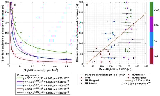
Figure 2.
(a) Flight-line density versus overall interpolation error; power regressions coloured to study sites. Black dotted line is the power-law model for all the interpolations and flight-line densities. (b) RMSD versus overall interpolation error for the various survey geometries; ordinary least squares linear regression plotted in red.
The increased prevalence of elevations with absolute DME values exceeding 500 m across the EGA led to a corresponding increase in interpolation errors (Figure 3). Compared with Kangerlussuaq, EGA interpolation errors from a 15 km spaced grid survey were typically one and a half times greater for the same Euclidean distance from inputs. Kangerlussuaq (Figure 3a,c) and the East Greenland Analogue (Figure 3b,d) are shown as end-member examples representing subdued and high-relief bed topographies, respectively. Furthermore, the estimated error from BedMachine was reduced in comparison with interpolation errors across the EGA for the first 2500 m from an input point; however, for Kangerlussuaq, BedMachine only provided reduced uncertainty estimates for the first 1300 m (Figure 3).
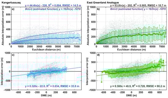
Figure 3.
Individual interpolation errors (shaded dots) vs. distance and DME for 15 km grid surveys over the Kangerlussuaq and EGA study sites. Moving means are every 150 m for distance and 10 m for DME (filled circles); error bars represent standard deviation in y and the moving mean window in x. Ordinary least squares regressions for the moving mean and error (solid lines) are described above the plot. (a) Kangerlussuaq: Euclidean distance versus interpolation error. (b) EGA: Euclidean distance versus interpolation error. (c) Kangerlussuaq: DME versus interpolation error. (d) EGA: DME versus interpolation error.
3.3. Individual Interpolation Errors for Kriged Subglacial Bed Topography
For individual interpolation errors, the Euclidean distance of an interpolated cell from an input did not correlate with the absolute error (R2 = 0.197). Furthermore, the Euclidean distance showed no correlation with the real value for the error. We found the correlation to strengthen when the mean interpolation error was computed for every 150 m of distance (Figure 3a: R2 = 0.884 and p = 4.27 × 10⁻³³; Figure 3b: R2 = 0.905 and p = 6.08 × 10−36; and Figure 4a: R2 = 0.952 and p = 6.60 × 10⁻³⁴). As the gridded output for our sites and BedMachine was posted at 150 m, no accuracy was lost by grouping distances into 150 m intervals. Notably, the mean interpolation errors were consistently below the function applied to the distance from an input for Bedmachine (Figure 4a, purple line). While some errors exceeded this, 91% fell below the function line. Accordingly, the function established from these results predicted reduced uncertainty for all interpolation locations further than 1600 m from an input location compared with BedMachine.
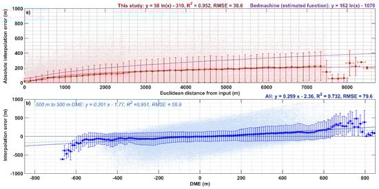
Figure 4.
All observations (shaded dots) of interpolation error versus Euclidean distance (a) and DME (b). Filled circles represent moving means, 150 m for distance and 10 m for DME; error bars represent standard deviation in y and the moving mean window in x. Ordinary least squares regressions calculated for the moving mean and error are described above the plots (solid lines and dashed light blue line in (b)).
Individually, the DME of an interpolation point did not correlate with the interpolation error at that point (Figure 4b). However, when grouped into 10 m intervals, the DME was a strong predictor of the interpolation error (R2 = 0.732; p = 4.27 × 10−46), albeit this sacrificed precision in the interpolated bed elevation (Figure 3c,d and Figure 4b). The DME performed more strongly in regions of subdued relief (e.g., Kangerlussuaq; Figure 3c: R2 = 0.834 and p = 2.27 × 10⁻³⁴), while in regions of heightened relief, its predictive strength was comparable to the overall model performance (e.g., EGA; Figure 3d: R2 = 0.728 and p = 2.31 × 10−39). Moreover, when locations with an absolute DME exceeding 500 m were removed due to their limited abundance in comparison with the rest of the data, the correlation strengthened, and the RMSE was reduced (R2 = 0.951; p = 2.29 × 10−68). For consistency, the function incorporating all the observations was used throughout. The DME provides a robust alternative estimate of error, as it is based on the topography of the interpolated dataset, as opposed to the distance from an input. As such, it can still be applied in sparsely surveyed areas. Additionally, the sign of the interpolation error can be determined, as opposed to just the absolute value. At a reduced flight-line density, the correlation between the DME and interpolation error strengthened (Table 1). For high-density surveys, no correlation existed, as the errors became more random, albeit significantly reduced (lower RMSE in Table 1).

Table 1.
Coefficients for DME–error functions for various flight survey geometries. Line survey coefficients are means with standard deviations for MP and MO, marginal and interior simulated surveys. M and C are the respective gradient and intercept constants of the best-fitting linear error function. The full results are presented in Table S2.
3.4. Application to BedMachine
When applied to the input flight-line coverage for BedMachine, our observation-based Euclidean distance versus interpolation error function provided a first-order error estimate for bed topography in the ice sheet interior (Figure 5). We found that the uncertainty in ice thickness and bed elevation measurements was reduced, on average, by 104 ± 174 m (~3% of the max. ice thickness). Uncertainties within one standard deviation of the predicted error were reduced for 67% of the kriged area of BedMachine (Figure 5b). For the 99% confidence interval (3σ), 37% of the area had lower estimates of error where our observation-based distance function was applied (Figure 5c). Importantly, substantial improvement, i.e., over 200 m of uncertainty reduction, occurred in areas where the flight-line density was exceedingly sparse (green regions in Figure 5).
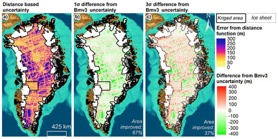
Figure 5.
Distance–error function from Figure 4. applied to the kriged areas of BedMachine [9]. (a) Derived uncertainty estimate. (b) Derived uncertainty plus one standard deviation differenced from Bedmachine uncertainty. (c) Derived uncertainty plus three standard deviations differenced from BedMachine uncertainty. Background colours depict topography: sea floor is shown in shades of blue (dark = low; light = high) and land surface in shades of brown (light = high; dark = low).
In regions with the lowest flight-line density (<0.1 lines km−2), we found the mean reduction in uncertainty was approximately 89 ± 235 m within one standard deviation and 12 ± 236 m for a 99% confidence interval (CI). However, as the sign of the interpolation error shows no relationship with distance, distance alone cannot predict whether the error is likely positive or negative. Additional information is required to predict whether the bed topography is expected to be lower or higher at a location.
As the 10 m moving mean DME correlated strongly with real values for the interpolation error, it could be used to apply a mean probable difference adaptation to the kriged areas of BedMachine, with associated confidence estimates (Figure 6). The mean for this difference was −5 ± 41 m, resulting in a deepening of the bed topography across the interior. Figure 5b shows the 99% CI for the absolute mean probable difference from the DME method. In locations with a survey density greater than 0.1 lines km−2, the BedMachine uncertainty was lower by 90 ± 114 m, whereas in areas with sparse flight-line coverage, the DME-based uncertainty was reduced (−29 ± 252 m).
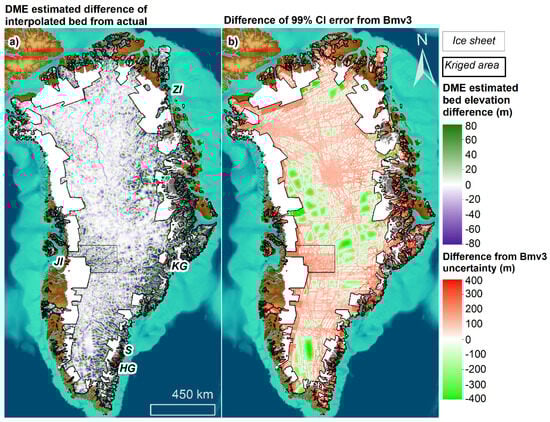
Figure 6.
The DME–error function applied to the kriged area of BedMachine. (a) The predicted mean difference in the bed elevation from the actual bed elevation. Outlet glaciers with extensive deepening in their interior portions are labelled (HG: Heimdal Glacier; JI: Jakobshavn Isbræ; KG: Kangerlussuaq; S: Skinfaxe; and ZI: Zachariae Isstrøm). (b) The predicted mean difference plus three standard deviations difference from Bedmachine uncertainty. Background colours depict topography: sea floor is shown in shades of blue (dark = low; light = high) and land surface in shades of brown (light = high; dark = low).
For areas of kriged bed topography where the flight-line density is less than 0.14 lines per km2, the DME method will provide lower estimates of uncertainty in subglacial topography than currently estimated (99% confidence interval; Figure 7). Such a flight-line density is equivalent to conducting a 3.5 km spaced grid or a 1.8 km spaced line survey. Approximately 56% of the interior of the GrIS is surveyed to this level. Furthermore, our method increasingly improves uncertainty estimates, relative to other datasets, with decreasing flight-line density. Conversely, for denser surveys, the method is less precise than the current estimates of uncertainty (Figure 5, Figure 6 and Figure 7). From this, the mean likely difference may be applied to kriged bed topography to deepen lowlands and raise highlands, addressing one of the main drawbacks of kriging [24], with an accompanying 99% confidence interval (Figure 6).
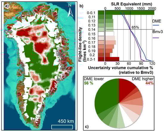
Figure 7.
Flight-line density within a 50 km search window (lines km−2) across the kriged area of BedMachine. (a) Mapped flight-line density, green shows where DME–error function is predicted to reduce uncertainty with respect to Bedmachine, and red is vice versa. (b) Bar chart shows the amount of sea-level rise (SLR) equivalent estimated in each region using BedMachine; lines show the cumulative percentage of the uncertainty volume (uncertainty in elevation multiplied by area) at each flight-line density for DME (blue) and BedMachine (purple). (c) Pie chart shows representative areas of each flight-line density class; the sum of green segments is the area where the DME uncertainty is likely to be lower than that for BedMachine. Background colours depict topography: sea floor is shown in shades of blue (dark = low; light = high) and land surface in shades of brown (light = high; dark = low).
4. Discussion
4.1. Recommendations for Future Survey Planning
The above results provide useful information for planning future RES surveys over ice masses in order to optimise the placement of survey lines to make the largest improvement to our knowledge of subglacial topography. For an assumed topographic setting akin to the ones investigated here, Figure 2 may be used to approximate the accuracy of an interpolated bed dataset from a given flight-line density. Our results also provide solutions for minimising uncertainty in outputs where sparse surveys are flown. Figure 7 highlights that this can be beneficial for large swathes of subglacial topography.
4.2. Uncertainty Improvement in Sparsely Surveyed Regions
In regions of low survey density, uncertainties in any bed topography dataset are greatest [7]. Firstly, our results show currently implemented distance–error functions overestimate the likely interpolation error at a given location; hence, we implemented a refined error estimate based on the results of the 1.5 million sample points taken in this study. Secondly, we proposed a method for obtaining significantly reduced uncertainty based on the bed topography estimate itself, constrained by knowledge of the elevation. This second uncertainty estimate sacrifices 10 m of accuracy in bed topography estimates to provide a probable difference at a location, which may be used to adapt the bed topography. Previous studies have reported bed elevation uncertainties of 20–70 m [36,37]; hence, a 10 m reduction in accuracy is well within the largely reported uncertainties in analysis derived from bed topography. As this method is expedient, it may be applied to kriged bed topography datasets as a quick and low-cost alternative to other methods.
Sparsely surveyed regions of the GrIS constitute large volumes of ice [1,9]. High uncertainties in these regions, therefore, have a greater effect on the overall estimate of volume for the ice sheet. Subsequently, this results in higher uncertainties in the potential future sea-level contribution from Greenland, and our method poses a means of reducing this. Furthermore, this approach may increase model performance over large areas of the ice sheet where bed topography uncertainty is significantly reduced [38]. Where our method deepens or raises the bed to its probable elevation consistently over long-wavelength features (continuous areas of deep purple and green in Figure 6), a significant improvement in model performance may be gained [38].
Our DME method can be efficaciously applied to approximately 56% of the kriged area of BedMachine, which equates to an area of 48% of the entire ice sheet. This area contains a potential global mean sea-level rise (SLR) contribution of 3.5 m, which equates to roughly 47% of the ice sheet total (7.4 m [9]). We estimate that the reduction in the uncertainty volume across this region, the area of the uncertainty in ice thickness multiplied by its scale, is equivalent to 8.5 centimetres of sea-level contribution (Figure 7). This estimate is conservative, as the above analysis is based on regions where the 99% confidence interval of our uncertainty can be expected to be lower than for Bedmachine. While this is a marked reduction in uncertainty, the regions in which our method is most effective are interior portions of the ice sheet that are unlikely to contribute to sea-level rise over the next centuries [39].
Uncertainty estimation for RES-derived bed elevation has evolved alongside interpolation methodologies. Deterministic approaches, such as inverse distance weighting or splines, are computationally efficient but perform poorly under the strongly anisotropic sampling geometry of RES data and provide limited uncertainty information [10,40]. Physically based mass conservation (MC) methods enforce flux balance to infer bed elevation [9], but their reliance on assumptions such as steady-state flow and fixed depth-averaged velocity relationships can lead to systematic biases, particularly in dynamically evolving regions [25]. Geostatistical approaches, notably kriging, explicitly model spatial covariance, accommodate directional sampling aligned with ice flow, and provide statistically rigorous uncertainty estimates [7]. However, kriging-derived uncertainties remain sensitive to variogram choice and sparse across-track sampling [7]. More recently, machine learning approaches, such as quantile regression forests (QRFs), have been proposed to generate data-driven predictive uncertainty by modelling full conditional distributions using auxiliary covariates [11], though their lack of explicit physical constraints can degrade performance in regions where strong prior information is not encoded in the model, such as hydrostatic equilibrium for regions of floating ice [11]. In contrast, the DME method presented here does not seek to produce an alternative bed elevation product but instead operates on existing kriging-derived bed topography datasets to diagnose and reduce conservative uncertainty where geometric and sampling constraints are well understood, making it particularly applicable to interior ice sheet regions and directly compatible with current ice sheet model initialisation practices.
4.3. Implications for the Stability of the GrIS Interior
Our approach generates a deeper and steeper bed topography across the GrIS interior, suggesting an inherently more dynamic system with a greater overall contribution to sea-level rise [28,41]. Moreover, we predict the current inland expanse of the GrIS below mean sea level may be 2% greater than previously reported [9]. Notably, areas of the ice sheet bed over 200 m below sea level were found to be nearly 30% more expansive (Figure 8 and Figure 9). An increase in the area below 200 m is important, as Atlantic water occurs at depths between 200 and 300 m [9,42,43]. Where this relatively warm water is able to reach Greenland outlet glacier margins, enhanced oceanic melting is expected [9,44], and areas of the ice sheet grounded below this depth and connected to the ocean are susceptible to its influence. Hence, if areas beneath 200 m below sea level are more expansive, as we predict, 30% more of the ice sheet interior becomes susceptible to the incursion of Atlantic water when the ice retreats into these locations. Additionally, increased depth below sea level combined with greater ice thickness brings the ice sheet closer to flotation, potentially enhancing future retreat due to reduced effective pressure at the grounding line [45,46]. As the interior of the ice sheet is strongly grounded, it is more sensitive to this effect [47].
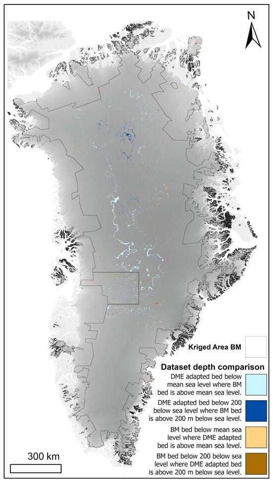
Figure 8.
BedMachine V3 (‘BM’; ref. [9]) and adapted kriged region bed topography depth differences. Blue shading indicates areas where the elevation in the adapted bed topography is lower than the specified threshold and above the threshold in BedMachine. Orange shading indicates the opposite. Lighter shading represents areas with a threshold at the global mean sea level, while darker shading represents areas 200 m below the global mean sea level.
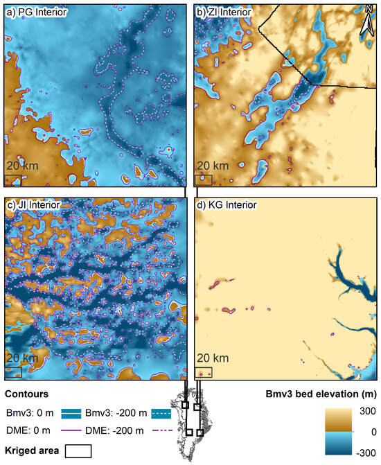
Figure 9.
Sub-sea-level contours for Bedmachine (white) and DME-adapted BedMachine subglacial elevation (purple). Dashed contours illustrate areas 200 m below sea level. (a) Interior area of the Petermann Glacier canyon and the ice sheet interior. (b) Interior area of Zachariae Isstrøm. (c) Jakobshavn Isbræ interior. (d) Kangerlussuaq glacier interior.
Although it can be reasonably assumed that neighbouring expanded deeper areas are connected, our results do not show this (Figure 8). As our results predominantly modified kriged bed topography in the vertical domain, they did not improve the horizontal connectivity of deep basins; hence, “bullseye”-like interpolation artefacts still exist in the dataset (Figure 8; ref. [24]), which remain a challenge for ice sheet modelling studies. While our method does not remove interpolation artefacts that hinder accurate numerical modelling [38], estimates of the sea-level rise contribution would still be greater than the unmodified dataset purely from the deepening of the bed [28]. Though the interior portion of the GrIS is unlikely to contribute to sea-level rise in the current century [39], these findings have implications for our appreciation of the stability of the GrIS in the far future [48]. Nevertheless, isostatic uplift of the bed with deglaciation will act to alleviate this, and it is uncertain how ocean temperature and circulation will evolve on these longer timescales [48].
4.4. Implications for the Stability of Greenland Outlet Glaciers
Our results suggest that the greatest differences in bed elevation are prevalent where the elevation is significantly above or below the local mean elevation. Therefore, where valley cross-sections are derived from the bed topography for ice discharge calculations, these calculations are likely underestimates. The valley cross-sectional area, widely used to calculate ice flux [49], was found to increase by 1 ± 1% if our DME-estimated elevation difference was applied (Figure 10 [locations shown in Figure 11]). Therefore, where flux-gates have been drawn from kriged bed topography, the cross-sectional area should be increased by one per cent. Additionally, the DME-estimated bed elevation across flux-gates at the downglacier edge of the kriged area (i.e., the transition zone to the mass conservation-derived bed topography) was found to be 7 ± 20% lower than in the original kriging (Figure 10), which has implications for the depth-averaged velocity parameter in ice discharge calculations [50].
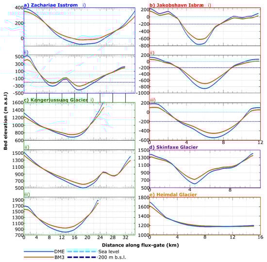
Figure 10.
Comparison of Bedmachine (orange profiles) and DME (blue profiles) altered flux-gate bed elevation cross-sections for major outlet glaciers (labelled in Figure 6). (a) Zachariae Isstrøm: (i) North and (ii) South; (b) Jakobshavn Isbræ: (i) North, (ii) Central, and (iii) South; (c) Kangerlussuaq Glacier: (i) North, (ii) Central, and (iii) South; (d) Skinfaxe Glacier; and (e) Heimdal Glacier.
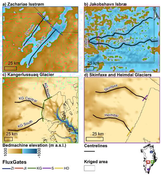
Figure 11.
Map of centreline and flux-gate bed elevation profile locations highlighted in Figure 10 and Figure 12. (a) Zachariæ Isstrøm flux-gate and centreline locations, (b) Jakobshavn Isbræ flux-gate and centreline locations, (c) Kangerlussuaq flux-gate and centreline locations, and (d) Skinfaxe and Heimdal flux-gate and centreline locations.
Flux-gate mean depths throughout the area of the bed topography generated by kriging were found to be deeper, on average, for eight of the ten outlet cross-sections, six of which were significantly deeper at a 95% confidence interval. Consequently, discharge through these regions will be underestimated in models evaluating future dynamic mass loss through these catchments as the ice sheet retreats into them [48]. Importantly, our method has the potential to improve bed topography by reducing the tendency of kriging to smooth out critical bed features, such as valleys and ridges, which steer ice flow. By doing so, we can reduce uncertainty in bed topography over large areas of the interior, enhancing future modelling efforts (Figure 5 and Figure 6). It has been found that a reduction in bed topography uncertainty over long-wavelength features significantly improves numerical modelling [38]. Perturbations of 10s of meters have been observed to strongly influence predicted grounding line retreat [38]. As we provide reduced uncertainty in bed topography and its likely difference (deeper or shallower), our method could be used to improve predictions of the evolution of the interior portions of the GrIS grounded below sea level.
The mean depth along the approximate centrelines of the interior portions of the outlet glaciers labelled in Figure 6 was found to be deeper by 86 ± 20 m (Figure 12). Importantly, for outlets with extensive sub-sea-level bed topography connected to the ice sheet interior (Zachariae Isstrøm and Jakobshavn Isbræ), retrograde bed slopes were found to be steeper by 0.3 ± 0.1° (or 0.5 ± 0.2 as a percentage slope; Figure 12). This is of crucial importance to our understanding of the stability of the GrIS, as sub-sea-level retrograde beds are potentially susceptible to MISI [51,52]. The same gradient increase was observed across all the sampled retrograde beds, suggesting gradients of such beds in other kriged bed topography datasets are likely underestimated. Additionally, the expanse of the area 200 m below sea level is observed across the subglacial topography for Petermann Glacier, Zachariae Isstrøm, and Jakobshavn Isbræ (Figure 11), which, when modelled, would increase the susceptibility of these glaciers to Atlantic water incursions and, consequently, their perceived stability [44]. Deepening of the bed also occurs at the interior of the southern branch of the Kangerlussuaq glacier, where a portion of the bed is lowered below sea level approximately 100 km from the margin along a retrograde bed slope, potentially increasing the susceptibility of this rapidly retreating portion of the ice sheet interior to enhanced retreat in the far term [52,53]. However, the connecting subglacial topography between the current sub-sea-level portion of the glacier and this upglacier section is well above sea level (Figure 11c). Hence, it is likely that inland retreat here will be reduced in the near term when the outlet retreats onto land. These glaciers comprise four of the eight largest contributors to ice discharge from the GrIS [54]. Consequently, long-term forecasts of their sensitivity to grounding line retreat may be underestimated.

Figure 12.
Comparison of BedMachine (orange profiles) and DME (blue profiles) altered centreline bed elevation cross-sections for major outlet glaciers (labelled in Figure 6). (a) Zachariae Isstrøm: (i) North and (ii) South; (b) Jakobshavn Isbræ: (i) North and (ii) South; (c) Kangerlussuaq Glacier: (i) North, (ii) Central, and (iii) South; (d) Skinfaxe Glacier; and (e) Heimdal Glacier.
5. Conclusions
We presented two methods for quantifying and reducing uncertainties in kriged subglacial bed topography datasets. Firstly, a revised distance–error function was presented, which reduces uncertainty in bed topography for areas located further than 1.5 km from flight-line observation. Secondly, an alternative method was presented to estimate the potential difference in subglacial elevation at an interpolated point from the bed elevation generated by kriging. We found that this method provides the greatest benefit in areas with flight-line densities sparser than a 3.5 km spaced grid or 1.8 km spaced parallel flight-lines, approximately 56% of the GrIS interior. Consequently, our method reduces uncertainty over an area of the interior that contains 65% of its ice volume. A reduction in uncertainty by up to hundreds of metres provides improved confidence in bed topography input conditions for numerical modelling of the GrIS [38].
Adaptation of the BedMachine Greenland v3 subglacial topography using our DME method resulted in the deepening of valleys and raising of highlands across the ice sheet interior. Elevation lowering in subglacial valley bottoms was more prevalent than elevation heightening, leading to a seven-millimetre increase in the potential global mean sea-level contribution from the GrIS. Moreover, the total area below sea level expanded by 2%. Of particular importance is that the area 200 m below sea level expanded by 29%. This improvement in the confidence of the area significantly below sea level is important for more reliably modelling the susceptibility of major outlet glaciers to enhanced grounding line retreat in the future, as the ice sheet retreats into these bed elevation lows [48]. Consequently, assessments of the future stability of the GrIS should account for the potential for a wider area of the bed to be susceptible to incursions of Atlantic Water [39]. Importantly, these regions contain three of the eight largest glaciers in terms of solid ice discharge from the ice sheet [54]. While the focus of this study was on the interior of the ice sheet, which has implications for long-term sea-level change [48], the connectivity of these interior regions to the ocean through major outlet glaciers like the Ilullissat Glacier (Jakobshavn Isbræ), which were found to have deeper and steeper retrograde beds, may have potential implications for rates of ice loss in the near term.
Finally, our method is based on observations over a wide suite of topographic settings expected to occur beneath any ice mass. As such, it may be applied to bed topography datasets for other ice masses, which are derived by kriging (e.g., Martian polar ice caps [55]). Consequently, this may contribute to reduced uncertainty in bed elevation for ice sheet model inputs and subsequent projections of sea-level change.
Supplementary Materials
The following supporting information can be downloaded at https://www.mdpi.com/article/10.3390/rs18010016/s1, Figure S1: (a) Kriged bed topography grids of the Inglefield Land PGA, (b) Kriged bed topography grids of the Kangerlussuaq PGA, (c) Kriged bed topography grids of the Peary Land PGA, (d) Kriged bed topography grids of the EGA PGA; Figure S2: Boxplot showing variation in interpolation quality as a result of survey geometry and proximity to the bed; Table S1: Kriging parameters for topographic grids generated for interpolation error assessment; and Table S2: Descriptive statistics for interpolation error based on input proglacial area and survey geometry.
Author Contributions
Conceptualization, O.T.B. and S.J.P.; Methodology, O.T.B.; Formal analysis, O.T.B.; Investigation, O.T.B.; Writing—original draft, O.T.B. and S.J.P.; Writing—review & editing, O.T.B. and S.J.P.; Supervision, S.J.P.; Funding acquisition, S.J.P. All authors have read and agreed to the published version of the manuscript.
Funding
This work was supported by the Natural Environment Research Council [grant number NE/L002434/1]. O.T.B. was funded by the NERC GW4+ DTP studentship NE/L002434/1. Geospatial support for this work was provided by the Polar Geospatial Center under NSF-OPP awards 1043681 and 1559691. DEMs were provided by the Polar Geospatial Center under NSF-OPP awards 1043681, 1559691, and 1542736.
Data Availability Statement
The ArcticDEM tiles used in this study are available via the Polar Geospatial Center [29]. The following tiles were used for the study areas investigated here: Inglefield Land, 29_36_2m_v3.0; Kangerlussuaq, 16_38_2m_v3.0; Peary Land, 31_44_2m_v3.0; and Mackenzie Mountains (EGA), 39_12_2m_v3.0. BedMachine v.3 is available from MM [9]. ArcMap 10.6 was used to conduct the spatial analysis in this research.
Acknowledgments
O.T.B. would like to acknowledge discussions with Anne Le Brocq, Neil Ross, and Mathieu Morlighem, which improved the communication and presentation of this study’s findings. The authors wish to thank the editors and two anonymous reviewers whose comments and feedback greatly improved this manuscript.
Conflicts of Interest
The authors declare no conflicts of interest.
References
- Bamber, J.L.; Griggs, J.A.; Hurkmans, R.T.W.L.; Dowdeswell, J.A.; Gogineni, S.P.; Howat, I.; Mouginot, J.; Paden, J.; Palmer, S.; Rignot, E.; et al. A new bed elevation dataset for Greenland. Cryosphere 2013, 7, 499–510. [Google Scholar] [CrossRef]
- Alley, R.B.; Clark, P.U.; Huybrechts, P.; Joughin, I. Ice-sheet and sea-level changes. Science 2005, 310, 456–460. [Google Scholar] [CrossRef]
- Schoof, C. Basal perturbations under ice streams: Form drag and surface expression. J. Glaciol. 2002, 48, 407–416. [Google Scholar] [CrossRef]
- Dowdeswell, J.A.; Evans, S. Investigations of the form and flow of ice sheets and glaciers using radio-echo sounding. Rep. Prog. Phys. 2004, 67, 1821. [Google Scholar] [CrossRef]
- Schroeder, D.M.; Bingham, R.G.; Blankenship, D.D.; Christianson, K.; Eisen, O.; Flowers, G.E.; Karlsson, N.B.; Koutnik, M.R.; Paden, J.D.; Siegert, M.J. Five decades of radioglaciology. Ann. Glaciol. 2020, 61, 1–13. [Google Scholar] [CrossRef]
- Rodriguez-Morales, F.; Gogineni, S.; Leuschen, C.J.; Paden, J.D.; Li, J.; Lewis, C.C.; Panzer, B.; Alvestegui, D.G.G.; Patel, A.; Byers, K.; et al. Advanced multifrequency radar instrumentation for polar research. IEEE Trans. Geosci. Remote Sens. 2013, 52, 2824–2842. [Google Scholar] [CrossRef]
- Bamber, J.L.; Layberry, R.L.; Gogineni, S.P. A new ice thickness and bed data set for the Greenland ice sheet: 1. Measurement, data reduction, and errors. J. Geophys. Res. Atmos. 2001, 106, 33773–33780. [Google Scholar] [CrossRef]
- Goff, J.A.; Powell, E.M.; Young, D.A.; Blankenship, D.D. Conditional simulation of Thwaites Glacier (Antarctica) bed topography for flow models: Incorporating inhomogeneous statistics and channelized morphology. J. Glaciol. 2014, 60, 635–646. [Google Scholar] [CrossRef]
- Morlighem, M.; Williams, C.N.; Rignot, E.; An, L.; Arndt, J.E.; Bamber, J.L.; Catania, G.; Chauché, N.; Dowdeswell, J.A.; Dorschel, B.; et al. BedMachine v3: Complete bed topography and ocean bathymetry mapping of Greenland from multibeam echo sounding combined with mass conservation. Geophys. Res. Lett. 2017, 44, 11051–11061. [Google Scholar] [CrossRef] [PubMed]
- Pritchard, H.D.; Fretwell, P.T.; Fremand, A.C.; Bodart, J.A.; Kirkham, J.D.; Aitken, A.; Bamber, J.; Bell, R.; Bianchi, C.; Bingham, R.G.; et al. Bedmap3 Updated Ice Bed, Surface and Thickness Gridded Datasets for Antarctica. Sci. Data 2025, 12, 414. [Google Scholar] [CrossRef]
- Palmer, S.; Kirkwood, C.; Luo, C.; Morlighem, M. A Quantile Regression Forest Estimate of Greenland’s Subglacial Topography. J. Glaciol. 2025, 71, e115. [Google Scholar] [CrossRef]
- Nowicki, S.M.; Payne, T.; Larour, E.; Seroussi, H.; Goelzer, H.; Lipscomb, W.; Gregory, J.; Abe-Ouchi, A.; Shepherd, A. Ice sheet model intercomparison project (ISMIP6) contribution to CMIP6. Geosci. Model Dev. 2016, 9, 4521. [Google Scholar] [CrossRef]
- Pritchard, H.D. Bedgap: Where next for Antarctic subglacial mapping? Antarct. Sci. 2014, 26, 742–757. [Google Scholar] [CrossRef]
- Lythe, M.B.; Vaughan, D.G. BEDMAP: A new ice thickness and subglacial topographic model of Antarctica. J. Geophys. Res. Solid Earth 2001, 106, 11335–11351. [Google Scholar] [CrossRef]
- Le Brocq, A.M.; Payne, A.J.; Vieli, A. An improved Antarctic dataset for high resolution numerical ice sheet models (ALBMAP v1). Earth Syst. Sci. Data 2010, 2, 247–260. [Google Scholar] [CrossRef]
- Fretwell, P.; Pritchard, H.D.; Vaughan, D.G.; Bamber, J.L.; Barrand, N.E.; Bell, R.; Bianchi, C.; Bingham, R.G.; Blankenship, D.D.; Casassa, G.; et al. Bedmap2: Improved ice bed, surface and thickness datasets for Antarctica. Cryosphere 2013, 7, 375–393. [Google Scholar] [CrossRef]
- Morlighem, M.; Rignot, E.; Binder, T.; Blankenship, D.; Drews, R.; Eagles, G.; Eisen, O.; Ferraccioli, F.; Forsberg, R.; Fretwell, P.; et al. Deep glacial troughs and stabilizing ridges unveiled beneath the margins of the Antarctic ice sheet. Nat. Geosci. 2019, 13, 132–137. [Google Scholar] [CrossRef]
- Morlighem, M.; Rignot, E.; Seroussi, H.; Larour, E.; Ben Dhia, H.; Aubry, D. A mass conservation approach for mapping glacier ice thickness. Geophys. Res. Lett. 2011, 38, L19503. [Google Scholar] [CrossRef]
- Morlighem, M.; Rignot, E.; Mouginot, J.; Seroussi, H.; Larour, E. Deeply incised submarine glacial valleys beneath the Greenland ice sheet. Nat. Geosci. 2014, 7, 418–422. [Google Scholar] [CrossRef]
- Sundal, A.V.; Shepherd, A.; Nienow, P.; Hanna, E.; Palmer, S.; Huybrechts, P. Melt-induced speed-up of Greenland ice sheet offset by efficient subglacial drainage. Nature 2011, 469, 521–524. [Google Scholar] [CrossRef]
- Davison, B.J.; Sole, A.J.; Cowton, T.R.; Lea, J.M.; Slater, D.A.; Fahrner, D.; Nienow, P.W. Subglacial drainage evolution modulates seasonal ice flow variability of three tidewater glaciers in southwest Greenland. J. Geophys. Res. Earth Surf. 2020, 125, e2019JF005492. [Google Scholar] [CrossRef]
- Deutsch, C.L.; Journel, A.G. GSLIB: Geostatistical Software Library and User’s Guide, 2nd ed.; Oxford University Press: Oxford, UK, 1997. [Google Scholar]
- Dowdeswell, J.A.; Benham, T.J.; Gorman, M.R.; Burgess, D.; Sharp, M.J. Form and flow of the Devon Island ice cap, Canadian Arctic. J. Geophys. Res. Earth Surf. 2004, 109, F02002. [Google Scholar] [CrossRef]
- Williams, C.N.; Cornford, S.L.; Jordan, T.M.; Dowdeswell, J.A.; Siegert, M.J.; Clark, C.D.; Swift, D.A.; Sole, A.; Fenty, I.; Bamber, J.L. Generating synthetic fjord bathymetry for coastal Greenland. Cryosphere Discuss. 2017, 11, 363–380. [Google Scholar] [CrossRef]
- Durand, G.; Gagliardini, O.; Favier, L.; Zwinger, T.; Le Meur, E. Impact of bedrock description on modeling ice sheet dynamics. Geophys. Res. Lett. 2011, 38, L20501. [Google Scholar] [CrossRef]
- Larour, E.; Seroussi, H.; Morlighem, M.; Rignot, E. Continental scale, high order, high spatial resolution, ice sheet modeling using the Ice Sheet System Model (ISSM). J. Geophys. Res. Earth Surf. 2012, 117, F01022. [Google Scholar] [CrossRef]
- Shepherd, A.; Ivins, E.; Rignot, E.; Fettweis, X. Mass balance of the Greenland Ice Sheet from 1992 to 2018. Nature 2019, 579, 233–239. [Google Scholar] [CrossRef] [PubMed]
- Nias, I.J.; Cornford, S.L.; Payne, A.J. New mass-conserving bedrock topography for Pine Island Glacier impacts simulated decadal rates of mass loss. Geophys. Res. Lett. 2018, 45, 3173–3181. [Google Scholar] [CrossRef]
- Claire, P.; Paul, M.; Ian, H.; Myoung-Jon, N.; Brian, B.; Kenneth, P.; Scott, K.; Matthew, S.; Judith, G.; Karen, T.; et al. ArcticDEM. Harvard Dataverse, V1. 2018. Available online: https://dataverse.harvard.edu/dataset.xhtml?persistentId=doi:10.7910/DVN/OHHUKH (accessed on 15 February 2020).
- Bartlett, O.T.; Palmer, S.J.; Schroeder, D.M.; MacKie, E.J.; Barrows, T.T.; Graham, A.G. Geospatial simulations of airborne ice-penetrating radar surveying reveal elevation under-measurement bias for ice-sheet bed topography. Ann. Glaciol. 2020, 61, 46–57. [Google Scholar] [CrossRef]
- Lindbäck, K.; Pettersson, R.; Doyle, S.H.; Helanow, C.; Jansson, P.; Kristensen, S.S.; Stenseng, L.; Forsberg, R.; Hubbard, A.L. High-resolution ice thickness and bed topography of a land-terminating section of the Greenland Ice Sheet. Earth Syst. Sci. Data 2014, 6, 331–338. [Google Scholar] [CrossRef]
- Jamieson, S.S.R.; Stokes, C.R.; Ross, N.; Rippin, D.M.; Bingham, R.G.; Wilson, D.S.; Margold, M.; Bentley, M.J. The Glacial Geomorphology of the Antarctic Ice Sheet Bed. Antarct. Sci. 2014, 26, 724–741. [Google Scholar] [CrossRef]
- Eyles, N.; Moreno, L.A.; Sookhan, S. Ice streams of the Late Wisconsin Cordilleran Ice Sheet in western North America. Quat. Sci. Rev. 2018, 179, 87–122. [Google Scholar] [CrossRef]
- Studinger, M.; Koenig, L.; Martin, S.; Sonntag, J. Operation Icebridge: Using Instrumented Aircraft to Bridge the Observational Gap between Icesat and Icesat-2. In Proceedings of the 2010 IEEE International Geoscience and Remote Sensing Symposium, Honolulu, HI, USA, 25–30 July 2010; pp. 1918–1919. [Google Scholar]
- Jezek, K.; Wu, X.; Paden, J.; Leuschen, C. Radar mapping of Isunnguata Sermia, Greenland. J. Glaciol. 2013, 59, 1135–1146. [Google Scholar] [CrossRef]
- Enderlin, E.M.; Howat, I.M.; Jeong, S.; Noh, M.J.; van Angelen, J.H.; van den Broeke, M.R. An improved mass budget for the Greenland ice sheet. Geophys. Res. Lett. 2014, 41, 866–872. [Google Scholar] [CrossRef]
- King, M.D.; Howat, I.M.; Jeong, S.; Noh, M.J.; Wouters, B.; Noël, B.; van den Broeke, M.R. Seasonal to decadal variability in ice discharge from the Greenland Ice Sheet. Cryosphere 2018, 12, 3813. [Google Scholar] [CrossRef]
- Sun, S.; Cornford, S.L.; Liu, Y.; Moore, J.C. Dynamic response of Antarctic ice shelves to bedrock uncertainty. Cryosphere 2014, 8, 1561–1576. [Google Scholar] [CrossRef]
- Calov, R.; Beyer, S.; Greve, R.; Beckmann, J.; Willeit, M.; Kleiner, T.; Rückamp, M.; Humbert, A.; Ganopolski, A. Simulation of the future sea level contribution of Greenland with a new glacial system model. Cryosphere 2018, 12, 3097–3121. [Google Scholar] [CrossRef]
- Peters, M.E.; Blankenship, D.D.; Carter, S.P.; Kempf, S.D.; Young, D.A.; Holt, J.W. Along-Track Focusing of Airborne Radar Sounding Data from West Antarctica for Improving Basal Reflection Analysis and Layer Detection. IEEE Trans. Geosci. Remote Sens. 2007, 45, 2725–2736. [Google Scholar] [CrossRef]
- Cornford, S.L.; Martin, D.F.; Payne, A.J.; Ng, E.G.; Le Brocq, A.M.; Gladstone, R.M.; Edwards, T.L.; Shannon, S.R.; Agosta, C.; van den Broeke, M.R.; et al. Century-Scale Simulations of the Response of the West Antarctic Ice Sheet to a Warming Climate. Cryosphere 2015, 9, 1579–1600. [Google Scholar] [CrossRef]
- Holland, D.M.; Thomas, R.H.; De Young, B.; Ribergaard, M.H.; Lyberth, B. Acceleration of Jakobshavn Isbræ triggered by warm subsurface ocean waters. Nat. Geosci. 2008, 1, 659–664. [Google Scholar] [CrossRef]
- Rignot, E.; Fenty, I.; Xu, Y.; Cai, C.; Velicogna, I.; Cofaigh, C.Ó.; Dowdeswell, J.A.; Weinrebe, W.; Catania, G.; Duncan, D. Bathymetry data reveal glaciers vulnerable to ice-ocean interaction in Uummannaq and Vaigat glacial fjords, west Greenland. Geophys. Res. Lett. 2016, 43, 2667–2674. [Google Scholar] [CrossRef]
- Schaffer, J.; Kanzow, T.; von Appen, W.J.; von Albedyll, L.; Arndt, J.E.; Roberts, D.H. Bathymetry constrains ocean heat supply to Greenland’s largest glacier tongue. Nat. Geosci. 2020, 13, 227–231. [Google Scholar] [CrossRef]
- Meier, M.F.; Post, A. Fast tidewater glaciers. J. Geophys. Res. Solid Earth 1987, 92, 9051–9058. [Google Scholar] [CrossRef]
- Stearns, L.A.; Van der Veen, C.J. Friction at the bed does not control fast glacier flow. Science 2018, 361, 273–277. [Google Scholar] [CrossRef]
- Favier, L.; Durand, G.; Cornford, S.L.; Gudmundsson, G.H.; Gagliardini, O.; Gillet-Chaulet, F.; Zwinger, T.; Payne, A.J.; Le Brocq, A.M. Retreat of Pine Island Glacier controlled by marine ice-sheet instability. Nat. Clim. Change 2014, 4, 117–121. [Google Scholar] [CrossRef]
- Aschwanden, A.; Fahnestock, M.A.; Truffer, M.; Brinkerhoff, D.J.; Hock, R.; Khroulev, C.; Mottram, R.; Khan, S.A. Contribution of the Greenland Ice Sheet to sea level over the next millennium. Sci. Adv. 2019, 5, eaav9396. [Google Scholar] [CrossRef]
- Shepherd, A.; Du, Z.; Benham, T.J.; Dowdeswell, J.A.; Morris, E.M. Mass balance of Devon Ice Cap, Canadian Arctic. Ann. Glaciol. 2007, 46, 249–254. [Google Scholar] [CrossRef]
- Van Wychen, W.; Burgess, D.O.; Gray, L.; Copland, L.; Sharp, M.; Dowdeswell, J.A.; Benham, T.J. Glacier velocities and dynamic ice discharge from the Queen Elizabeth Islands, Nunavut, Canada. Geophys. Res. Lett. 2014, 41, 484–490. [Google Scholar] [CrossRef]
- Schoof, C. Ice sheet grounding line dynamics: Steady states, stability, and hysteresis. J. Geophys. Res. Earth Surf. 2007, 112, F03S28. [Google Scholar] [CrossRef]
- Durand, G.; Gagliardini, O.; De Fleurian, B.; Zwinger, T.; Le Meur, E. Marine ice sheet dynamics: Hysteresis and neutral equilibrium. J. Geophys. Res. Earth Surf. 2009, 114, F03009. [Google Scholar] [CrossRef]
- Brough, S.; Carr, J.R.; Ross, N.; Lea, J.M. Exceptional Retreat of Kangerlussuaq Glacier, East Greenland, between 2016 and 2018. Front. Earth Sci. 2019, 7, 123. [Google Scholar] [CrossRef]
- Mankoff, K.D.; Colgan, W.; Solgaard, A.; Karlsson, N.B.; Ahlstrøm, A.P.; Van As, D.; Box, J.E.; Khan, S.A.; Kjeldsen, K.K.; Mouginot, J.; et al. Greenland Ice Sheet solid ice discharge from 1986 through 2017. Earth Syst. Sci. Data 2019, 11, 769–786. [Google Scholar] [CrossRef]
- Holt, J.W.; Fishbaugh, K.E.; Byrne, S.; Christian, S.; Tanaka, K.; Russell, P.S.; Herkenhoff, K.E.; Safaeinili, A.; Putzig, N.E.; Phillips, R.J. The construction of chasma boreale on Mars. Nature 2010, 465, 446–449. [Google Scholar] [CrossRef] [PubMed]
Disclaimer/Publisher’s Note: The statements, opinions and data contained in all publications are solely those of the individual author(s) and contributor(s) and not of MDPI and/or the editor(s). MDPI and/or the editor(s) disclaim responsibility for any injury to people or property resulting from any ideas, methods, instructions or products referred to in the content. |
© 2025 by the authors. Licensee MDPI, Basel, Switzerland. This article is an open access article distributed under the terms and conditions of the Creative Commons Attribution (CC BY) license.