Soil Organic Carbon Assessment Using Remote-Sensing Data and Machine Learning: A Systematic Literature Review

Abstract

In the current global change scenario, valuable tools for improving soils and increasing both agricultural productivity and food security, together with effective actions to mitigate the impacts of ongoing climate change trends, are priority issues. Soil Organic Carbon (SOC) acts on these two topics, as C is a core element of soil organic matter, an essential driver of soil fertility, and becomes problematic when disposed of in the atmosphere in its gaseous form. Laboratory methods to measure SOC are expensive and time-consuming. This Systematic Literature Review (SLR) aims to identify techniques and alternative ways to estimate SOC using Remote-Sensing (RS) spectral data and computer tools to process this database. This SLR was conducted using Systematic Review and Meta-Analysis (PRISMA) methodology, highlighting the use of Deep Learning (DL), traditional neural networks, and other machine-learning models, and the input data were used to estimate SOC. The SLR concludes that Sentinel satellites, particularly Sentinel-2, were frequently used. Despite limited datasets, DL models demonstrated robust performance as assessed by R2 and RMSE. Key input data, such as vegetation indices (e.g., NDVI, SAVI, EVI) and digital elevation models, were consistently correlated with SOC predictions. These findings underscore the potential of combining RS and advanced artificial-intelligence techniques for efficient and scalable SOC monitoring.

1. Introduction

Soil is the main life-supporting ecosystem service, as it supports plant growth, which is essential for human food and animal feed (provision services), as well as water retention, erosion control, and biodiversity (regulating services) [1]. Therefore, it is essential to understand the processes in the soil in order to develop sustainable use and management practices [2].

According to Pribyl [3], Soil Organic Carbon (SOC) constitutes approximately 58% of Soil Organic Matter (SOM) and plays an important role in water retention [4], soil fertility, and aggregate stabilization [5], being one of the main indicators of healthy soil and desertification [6], but also in monitoring the Carbon (C) stock of the soil, which is highly variable in space and time [7,8], which contributes to mitigating climate change [9,10].

Routine laboratory analyses commonly used to quantify SOC include SOM calcination, C chemical oxidation with oxidizing reagents such as chromium (Walkley–Black method) [11], or elemental chemical analysis [12]. However, these analyses are expensive, time-consuming, and require chemical reagents that generate toxic environmental waste [13]. Therefore, developing non-degradative techniques to reduce this environmental risk is extremely necessary [14].

Spectroscopic techniques are rapid, easy to use, less expensive, non-destructive, cost-efficient, and sometimes produce more reproducible data than conventional analysis in addition to the simultaneous characterization of soil properties (e.g., SOC, clay, and iron oxides). Although low-cost field equipment is currently available [14,15], these could present inaccuracies when variations occur in the surface layer of the soil due to roughness [16]. In a 2020 review paper by Odebiri et al. [17] on Remote Sensing (RS), 48% of the selected articles used a field spectrophotometer for SOC estimation using Machine Learning (ML). However, their research highlighted that satellite data had great potential to improve and facilitate SOC estimation, which is currently happening.

In recent decades, several studies have considered the advantages of RS, such as the ease of acquiring data, high revisit rate, and the possibility of working with large areas compared to traditional approaches [18,19,20,21,22,23]. However, RS spectra data processing presents some challenges, including dimensionality, spatiotemporal and spectral information, and numerous spectral bands [17].

In the last ten years, due to advances in computational processing and the development of metric techniques such as Traditional Neural Networks (TNNs) and Deep Learning (DL), there has been a rapid increase in studies related to RS data manipulation [24]. Some studies evaluate different TNN models to determine SOC content [25,26,27,28,29]. TNNs are capable of estimating SOC under different land conditions. However, their robustness is lower than that of DL approaches because they have few layers, restricting their ability to process complex data [30]. Therefore, the study and development of DL models has become even more crucial, as they present promising perspectives that have not yet been fully explored [17,31]. TNN and DL are highly related as DL is a subset of TNNs, yet TNNs are the fundamental building blocks with varying depths. In contrast, DL focuses on using Deep Neural Networks (DNNs) with multiple hidden layers for complex pattern recognition and representation.

This study aims to present and discuss the outcomes of a literature review focused on different methodologies for large-scale SOC estimates, using advanced computational techniques (TNN and DL) to process data obtained with non-invasive approaches (satellite imagery, field spectroscopic data, airborne or UVA data), alone or combined with other data sources, and highlights input data and algorithms for the best-performing SOC estimations.

2. Research Method and Literature Search

The methodology used is based on the Systematic Literature Review (SLR) by Kitchenham [32], whose main objective is to systematically identify, evaluate, and interpret all available data, filtering and extracting important information from a scientific area, after setting up all the literature’s inconsistencies, gaps, and limitations. Performing an SLR comprises three phases [33,34,35,36]—planning, conducting, and reporting—all of which will be described in the following sections. Before starting, the existence of other bibliographic reviews should be checked, being that if another recent work is found with the same research object, it is not pertinent to carry out another one [33,34,35,36,37,38].

2.1. Planning

The planning phase involves the development of a protocol that will facilitate the SLR conduction phase, aimed at the search objective. This phase includes elaborating questions, keywords, search strings, data sources, and selection criteria. One of the most important steps is formulation clear and focused research questions. These questions must be formulated to produce answers that provide the information intended to be discovered. Furthermore, these issues must be closely linked to the overall objectives of the review [35].

In addition to the protocol, the planning phase contains two more steps: quality criteria and data extraction. All these steps will be explained in the following sub-sections.

2.1.1. Research Questions

Compiling research questions is the first step in the planning phase. Precisely for this work, the objective is to identify which inputs by RS and which main DL and TNN models are used to estimate SOC. After identifying the objective, the following research questions were created:

• RQ1: What is the ideal study area size and number of samples that best predict SOC at a large scale?
• RQ2: What spectral data were used and what was their spatial and spectral resolution?
• RQ3: Which input data have more correlation with SOC?
• RQ4: What type of model (Other ML (O-ML), TNN, or DL) shows better results in SOC estimation?

2.1.2. Keywords and Synonyms

Keywords and synonyms are related to the main search terms. As the work deals with specific ML techniques (i.e., DL and TNN) used to estimate SOC through RS, the keywords and synonyms chosen for this research are shown in Table 1.

Table 1. Keywords and synonyms for the SLR.

Keywords	Synonyms
Deep Learning	Neural Network
Remote Sensing	-
Soil Organic Carbon	Organic Matter

2.1.3. Search String and Data Sources

Two databases were used for this work: Scopus and Web of Science (WoS).

A base search string was created according to the keywords previously defined. The criteria for its assembly were that each keyword in Table 1, or its synonym, should be included in the title, abstract, or keywords of the articles researched. Therefore, the base string was ((“deep learning” OR “neural network”) AND (“remote sensing”) AND (“soil organic carbon” OR ”organic matter”)).

Following the particularities of the websites of the selected databases, assigning the proposed criteria, the strings were as follows:

Two previous reviews on the same topic were found in research related to this SLR, with one being a detailed version and the other a summary that selected 95 studies for investigation [17,31]. Since these previous reviews covered the period up to 2020, this work includes an SLR from 2021 to 2023.

2.1.4. Selection Criteria

After the previous step, the inclusion or exclusion criteria assist in the orderly selection of these files. Even if an article is relevant, it must be eliminated if it contains one of the exclusion criteria. In this study, the inclusion criteria were all articles that were not in the exclusion criteria, which were as follows: it is not an article; it does not include advanced ML techniques (DL and TNN); it is not about SOC; it is not accessible; it is not written in English.

2.1.5. Quality Assessment Checklist

At this stage, new questions are elaborated to verify the quality and adequacy of an article with the SLR theme. Each question has a weight, and the answer value can be two values (zero = it answers nothing about the question, or one = it answers fully), reaching a maximum score of five. For an article to be considered suitable for SLR, it was defined that it would need to achieve a score of at least four. The five quality questions created are presented below:

• QQ1: Is there a clear objective of the research?
• QQ2: Are the work results discussed well?
• QQ3: Is it a research paper?
• QQ4: Is the work based on one or more DL/TNN models for SOC/SOM prediction?
• QQ5: Does the work use RS to predict SOC/SOM?

2.1.6. Data Extraction

The last step in the planning phase is to apply a data extraction form. In this stage, new questions are created to extract relevant data and information from the final articles selected in the previous stages. The data extraction questions formulated for this review were as follows:

• EQ1: What is the total size of the study area (km²)?
• EQ2: How many SOC samples were used?
• EQ3: What input data are used in the model?
• EQ4: Which input data correlated highest with SOC/SOM?
• EQ5: In the case of satellite imagery, what satellite was used, and what was its spatial and spectral resolution?
• EQ6: In the case of non-satellite image data, what is the source, and what is its spatial and spectral resolution?
• EQ7: What DL/TNN model was used to predict SOC/SOM?
• EQ8: What is the evaluation methodology?
• EQ9: Which DL/TNN model performed better (prediction model)?
• EQ10: Did the literature use temporal series to estimate SOC?

2.2. Conducting

The Preferred Reporting Items for Systematic Review and Meta-Analysis (PRISMA) protocol was used in the conducting phase. This method describes the methodology for carrying out SLRs [39,40].

The SLR conducting process, considering the PRISMA method, contains four steps: (1) “Identification”: search for articles in data sources; (2) “Screening”: the article’s title, abstract, and keywords must be read and those that do not meet the requirements are removed; (3) “Eligibility”: the suitable works were fully read and assessed the answers to the quality questions that generated a final score, and those that did not have a final score above three were excluded; (4) “Included”: extraction questions were applied. The relevant information is extracted from the literature found [39]. The Parsifal free platform was used for this SLR that, in addition to covering the entire step-by-step process of the PRISMA method, generates automatic reports and graphs.

2.3. Data Processing

The data collected in the previous steps were treated statistically using the Stat-graphics software. As there were quantitative and qualitative data, the last received binary values. The data were separated into platform type used (field spectrophotometer, satellite, drone, crewed aircraft), type of satellite, bands used, and type of resolution; vegetation, soil data, and topographic indices; and type of Artificial-Intelligence (AI) model, density sample, among others. This table is available as an appendix. The frequency and percentage of use were verified for each qualitative variable. The density sample variable was transformed into logarithmic for better data interpretation.

2.4. Reporting

The last phase of an SLR is the results dissemination report.

3. Results

In this section, the results obtained during the SLR are presented in the flowchart shown in Figure 1.

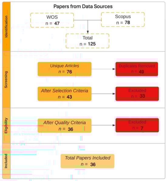
Figure 1. Conducting stage results of the systematic literature review.

In the identification stage, the search carried out in the databases identified 125 articles, 47 in WoS (37.6%) and 78 in Scopus (62.4%). During this process, 49 duplicate articles were removed, resulting in 76 unique articles. Subsequently, the inclusion and exclusion criteria were applied to the remaining articles in the screening stage. As a result, 43 articles met the requirements and advanced to the next phase, while 33 were excluded due to one or more established exclusion criteria. Seven were excluded in the eligibility stage, where all articles were read in full, leaving 36 works classified to the data extraction phase and used in the final review.

In Appendix A, Table A1 presents detailed information on these articles that underwent quality assessment, showing the answers suggested by the authors to the quality questions and the final grades assigned to each work. It is observed that most articles obtained maximum marks (five), which indicates that all items included in the review, besides being entirely related to the research topic, were also of good scientific quality. The only articles that did not obtain the maximum score were [41,42,43,44,45]; however, these articles were considered for the review. It was observed that the number of articles on the topic has grown in the last few years: of the 36 articles selected, 6 were from 2021, 16 from 2022, and 14 from 2023.

As for the countries where the studies were conducted, the results of the 2020–2023 review are similar to those of previous reviews [17,31]. That is, the review included studies that were carried out in 13 different countries: 16 works conducted in China; 6 in Iran; 3 in South Africa, 2 in the United States and Morocco; and 1 each in Kenya, India, Turkey, Lithuania, Italy, France, Portugal, and Spain (Figure 2).

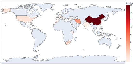
Figure 2. Number of research studies by country.

3.1. Data Extraction Questions

3.1.1. Study Area and SOC Samples (EQ1 and EQ2)

As most AI models based on Neural Networks (NNs) are fed back with real data of the variable to be modeled, in this case, the SOC, this review analyzed whether or not the number of SOC data (number of soil samples), the sampling surface, and density (number of samples/surface) were determining variables in the AI model section.

Figure 3 represents the SOC data used in each reviewed article, with the mean value being 1513 samples, a median of 249 samples, and a standard deviation of 6115.

There are some works with more than 1900 soil samples, including data from repositories or data available in databases. For example, Odebiri et al. [46,47,48] utilized the World Soil Information Repository (ISRIC). The red bar represents the work of S. Wang et al. [45], who used a substantial number of soil samples (37,540 points), being out of the scale of the other reviewed works, which used data from the Rapid Assessment Carbon (RaCA) repository, from the United States Department of Agriculture (USDA).

Regarding the surface area represented by the data collected in each article, some authors report large sampling areas with more than one million km² [45,46,47,48,49]. In contrast, other works apply AI models to relatively small areas, less than 50 km² [50,51,52,53,54,55,56]. In some cases, the authors do not identify the size of the study area but only its spatial location [41,44,57,58,59,60,61]. Based on the number of SOC samples and sampling area, the sampling density is calculated and expressed as the number of samples per area (Figure 4). L. Zhang et al. [62] also used this approach. It was impossible to obtain the sampling density for articles that did not present data from the study area, so they are not included in Figure 4.

The results show that, in most of the analyzed studies, the sampling density is less than one (i.e., less than one sample per km²). Among the studies that exceed this average value, three present densities lower than three samples per km², two are between 20 and 30 samples per km², and another three present more than 60 samples per km². One reviewed article stands out significantly, with a sampling density of 393.333 samples per km², much higher than the other reviewed articles, even higher than the studies that, although with many samples, present low sampling density. Since the sampling density data do not present a normal distribution, it was decided to transform them to a logarithmic scale. Figure 5 represents the frequency histogram (a) and variability of these data (b), on the logarithmic scale. The box and whisker graph highlights the median with a value close to zero, with a significant variation. The histogram shows a greater concentration of data around negative values, which suggests a tendency for lower sampling densities. The statistical analysis shows that the standard skewness and kurtosis are within the expected values for a normal distribution.

Figure 3. Number of samples used in each research (Mallik et al. (2022) [63], Gadal et al. (2023) [43], Liu et al. (2022) [51], Budak et al. (2023) [64], Y. Zhang et al. (2023) [59], Zayani et al. (2023) [56], Ou et al. (2021) [65], Salani et al. (2023) [66], Zeraatpisheh et al. (2021) [53], X. Wang et al. (2021) [52], Zolfaghari Nia et al. (2022) [58], Shi et al. (2021) [42], Chang et al. (2022) [41], F. Zhang et al. (2022) [44], Pellikka et al. (2023) [60], Fathizad et al. (2022) [67], K. Wang et al. (2021) [68], Xu et al. (2023) [57], Taghizadeh-Mehrjard et al. (2022) [69], L. Zhang et al. (2022) [62], Hosseini et al. (2023) [70], Abdoli et al. (2023) [71], Bouasria et al. (2022) [72], Li et al. (2021) [73], Samarinas et al. (2023) [74], Yang et al. (2022) [49], Guo et al. (2023) [61], Ma et al. (2022) [75], Meng et al. (2022) [50], Morais et al. (2023) [55], Li et al. (2023) [54], Zeng et al. (2022) [76], Odebiri et al. (2022a) [48], Odebiri et al. (2022b) [47], Odebiri et al. (2023) [46], S. Wang et al. (2022) [45]). (Note: The red bar does not correspond numerically to the x-axis).

Figure 4. SOC field sample density distribution by research (Yang et al. (2022) [49], Odebiri et al. (2022b) [47], Odebiri et al. (2022a) [48], Odebiri et al. (2023) [46], S. Wang et al. (2022) [45], Samarinas et al. (2023) [74], Fathizad et al. (2022) [67], L. Zhang et al. (2022) [62], Abdoli et al. (2023) [71], K. Wang et al. (2021) [68], Salani et al. (2023) [66], Hosseini et al. (2023) [70], Ma et al. (2022) [75], Gadal et al. (2023) [43], Li et al. (2021) [73], Zeng et al. (2022) [76], Budak et al. (2023) [64], Mallik et al. (2022) [63], Ou et al. (2021) [65], Bouasria et al. (2022) [72], Shi et al. (2021) [42], Zeraatpisheh et al. (2021) [53], Taghizadeh-Mehrjard et al. (2022) [69], Liu et al. (2022) [51], Meng et al. (2022) [50], Zayani et al. (2023) [56], X. Wang et al. (2021) [52], Li et al. (2023) [54], Morais et al. (2023) [55]).

Figure 5. Sample density analysis: (a) Frequency histogram and (b) Box plot (the orange line represents the median of the data).

3.1.2. Input Data (EQ3, EQ4, and EQ10)

The revised articles contain various input data for the models (data inputs), including RS data and topographic or environmental variables. Data inputs are critical to accurate SOC modeling as they capture essential aspects of land use, topography, vegetation, and climatic conditions that influence SOC distribution.

Figure 6 shows the different input data modalities to develop AI models, up to a total of 9 types (Spectral Data (Satellite Images, Vegetation and/or soil index, Field Spectrophotometer, Airborne image, Unmanned Aerial Vehicle (UAV) image), Topography (Digital Elevation Models—DEM), Climate, Soil properties, Land use, Vegetation parameters, Forest type, Geology, and Soil class), as well as the number of articles using each type.

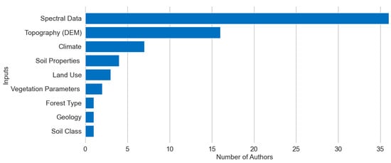
Figure 6. Variables used by the authors as input data for AI models for SOC.

Most authors use spectral data from satellite images, field spectrophotometes, or spectral indices calculated from spectral bands (such as Normalized Difference Vegetation Index (NDVI), Enhanced Vegetation Index (EVI), and others).

Most authors use accurate topographic data from DEM and some use more specific data. For example, Zeraatpisheh et al. [53] were unique in incorporating geological data, soil classes, and soil properties. Pellikka et al. [60] focused on vegetation parameters such as aboveground biomass and forest canopy height and density as inputs to their model, while L. Zhang et al. [62] used plant phenology data. Furthermore, only four authors employed aircraft with attached sensors to obtain spectral data [51,59,60,65]. Among them, Y. Zhang et al. [59] were the only ones to use a UAV. The authors, according to their specific needs, opted for different RS technologies to improve their SOC estimates. These technologies present different spatial, temporal, and spectral resolution characteristics, significantly affecting the estimates’ quality and precision and the costs and resources necessary for their implementation. In this sense, Figure 7 shows the percentage of RS platforms most used by authors.

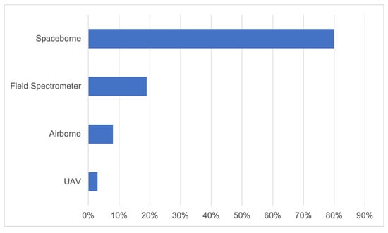
Figure 7. Remote-sensing platforms: frequency of use among researchers.

Figure 7 indicates that satellite data are the most popular platform among reviewed articles, used in 80% of reviewed articles. The field spectrophotometer appears in second place, with 19%. On the other hand, drones are the least used platform, with 3% of items using them. Although the figure does not present these data, some authors combined data from multiple platforms [50,51,56,57].

Derived from spectral bands in different spectrum regions (Visible (VIS), Near-Infrared (NIR), and Shortwave Infrared (SWIR)), vegetation and soil indices are the second most used types of data (Figure 6). Figure 8 details the most frequently used spectral indices in the articles included in this review. The NDVI is used in more than 60% of the articles, probably due to its simplicity of calculation and high correlation with green biomass [77], which is highly related to carbon in the soil [46,48,57,67]. Additionally, the NDVI is well-established and widely validated, providing confidence in the results [78]. The EVI, the Ratio Vegetation Index (RVI), and the Soil-adjusted Vegetation Index (SAVI) appear in more than 40% of the studies. Furthermore, the Difference Vegetation Index (DVI), Transformed Vegetation Index (TVI), and Brightness Index (BI) are used in a further 20% of the articles.

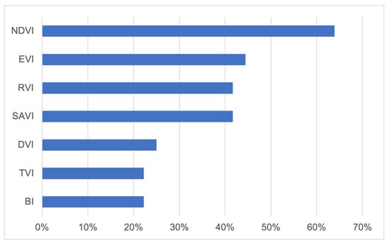
Figure 8. Main vegetation and soil indices used by researchers.

Some topographic indices obtained from the DEM, such as elevation, slope, and roughness, stand out as the input data most correlated with the SOC. However, several other indices also were used as inputs for AI models. The most used ones are shown in Figure 9.

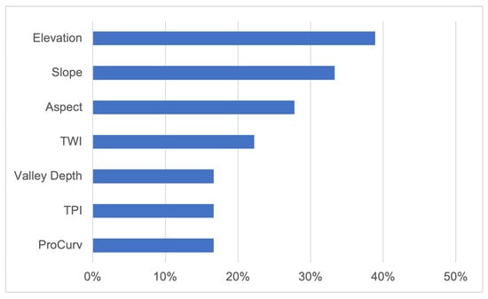
Figure 9. Frequency of use of topographic indexes by articles selected for this systematic literature review.

3.1.3. Satellite and Imagery Resolution (EQ 5 and EQ 6)

Among the five types of satellite data resolution are the following [79]: (1) spatial resolution: distance or pixel size, usually in meters per pixel (m/px); (2) temporal resolution: number of images of the exact location at the same time (number/days); (3) spectral resolution: number of spectral bands from visible-infrared-radar electromagnetic spectrum, each of which corresponds with a specific wavelength; (4) radiometric resolution: bytes of information; and (5) angular resolution, the spatial resolution is the one of greatest interest in this type of determinations.

Articles that used satellite image data or DEM are listed in Table 2, which details the equipment and spatial resolution used. In some cases, the authors resorted to resampling techniques to adjust the spatial resolution of the spectral bands to standardize them or to enhance the quality of images by rearranging the pixels of the original images. This is because satellite sensors have different spectral bands (e.g., Sentinel-2 has spatial resolution differences between bands: Band 1 and 10–11 (60 m); Band 5–7, 9, and 12–13 (20 m); and Band 2–4, and 8 (10 m) [79].

Table 2. Satellites type and spatial resolutions used in each article.

Reference	Satellite	Spatial Resolution
Odebiri et al. [46]	Sentinel-3 * SRTM	Original (300 m) Resampled to 300 m
Odebiri et al. [47]	Sentinel-3	Original (300 m)
Odebiri et al. [48]	Sentinel-3	Original (300 m)
Zeraatpisheh et al. [53]	Sentinel-2 Landsat 8 * ALOS	All resampled to 30 m
Xu et al. [57]	Sentinel-2 * ASTER GMDEM	All resampled to 10 m
L. Zhang et al. [62]	MODIS * Geomorpho90m	Resampled to 90 m Original (90 m)
Abdoli et al. [71]	Sentinel-2 Sentinel-3 Landsat 8 MODIS	Original (10 and 20 m) Original (300 m) Original (30 m) Original (250 m)
Zolfaghari Nia et al. [58]	Sentinel-2 Landsat 8	All resampled to 30 m
Liu et al. [51]	Sentinel-2	Resampled to 20 m
Meng et al. [50]	Landsat 8 GF-5 * SRTM	Original (30 m) Original (30 m) Original (30 m)
Fathizad et al. [67]	Landsat 5 Landsat 7 Landsat 8	Original (30 m) Original (30 m) Original (30 m)
K. Wang et al. [68]	Sentinel-2	Resampled to 20 m
Li et al. [73]	GF-1 * Cartosat-1 (IRS P5)	All resampled to 10 m
Zeng et al. [76]	Landsat 5 * SRTM	Original (30 m) Original (30 m)
Li et al. [54]	Sentinel-2 * NASA Earth Science Data	Resampled to 10 m Original (12.5 m)
Bouasria et al. [72]	Landsat 8	Resampled to 15 m
X. Wang et al. [52]	Sentinel-2	Resampled to 10 m
Taghizadeh-Mehrjardi et al. [69]	Landsat 8	Original (30 m)
Gadal et al. [43]	Landsat 5 Landsat 8 * ASTER GDEM	Original (30 m) Original (30 m) Original (30 m)
Mallik et al. [63]	Sentinel-2 * USGS	Original (10 and 20 m) Resampled to 10 m
Yang et al. [49]	Sentinel-2	Resampled to 20 m
Budak et al. [64]	Sentinel-2	Resampled to 10 m
Guo et al. [61]	Landsat 8 * ASTER GDEM	Original (30 m) Original (30 m)
Morais et al. [55]	Sentinel-1 Sentinel-2 * NASA EOSDIS	Original (10 m) Original (10 and 20 m) Original (30 m)
Samarinas et al. [74]	Sentinel-2	Resampled to 10 m
Salani et al. [66]	PRISMA	Original (30 m)
Hosseini et al. [70]	Landsat 8	Original (30 m)
Zayani et al. [56]	Sentinel-1 Sentinel-2	All resampled to 10 m

* Represents DEM.

The most used satellites were the Sentinel satellites, which belong to the Earth Observation Program of the European Space Agency (The Copernicus program, ESA), specifically the free open-access satellites Sentinel-2 and Sentinel-3 (Figure 10 and Figure 11). Moreover, the Landsat collection, specifically Landsat 7 and Landsat 8, developed by NASA in collaboration with the United States Geological Survey (USGS), was also evidenced in the review made by Velastegui-Montoya et al. [80] on the satellites most used in work using the Google Earth Engine tool.

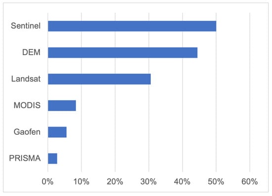
Figure 10. Satellite collection frequency use by researchers.

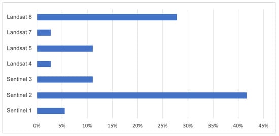
Figure 11. Airborne mission frequency use by researchers.

Regarding the DEM, as shown in Table 2, the Shuttle Radar Topography Mission (SRTM) led by NASA in the year 2000, with a spatial resolution of 30 m, was the most used [46,50,63,76]. Li et al. [54] and Morais et al. [55] only indicate that they used DEM from the NASA Earth data website with a spatial resolution of 12.5 and 30 m, respectively.

The spatial resolutions used by the authors were all above 10 m, as shown in Table 2. Some authors used the original spatial resolution of the data, while others resampled the data at the modified resolution. Considering the surfaces of the study areas, the spatial resolutions offer a good level of detail, even for Liu et al. [51], who used a study area of 2 km². Figure 12 shows the spatial resolutions used in the reviewed articles. Many works simultaneously used data with different pixel sizes, the spatial resolution most used being between 10 and 30 m, which explains why the sum of the bar percentages in Figure 12 exceeds 100%.

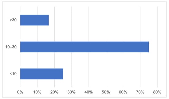
Figure 12. Distribution of the use of spatial resolutions in selected scientific studies.

Regarding the spectral resolution, even if the band numbers do not coincide, the bands can be compared to each other due to the spectral region they cover (for example, Band 8 Sentinel-2 corresponds to the same spectral region as Band 5 on Landsat 8). In general, spectral bands can be classified depending on the spectral region: UV (<400 nm), VIS (400–700 nm), NIR (700–1200 nm), SWIR (1200–2500 nm), and Thermal Infrared (TIR) (8000–14,000 nm) [79]. Figure 13 shows the bands used in the different articles. The VIS and NIR bands, which detect information mainly from vegetation or land use cover [79], are the most frequently used bands for SOC modeling (80%), while the UV bands are only used by 67% of users. The SWIR spectral region is also widely used, as it allows the detection of cover moisture content [79]. The TIR bands are widely used to detect vegetation evapotranspiration and material thermal properties [79]. However, this region was the least used for modeling SOC (28%).

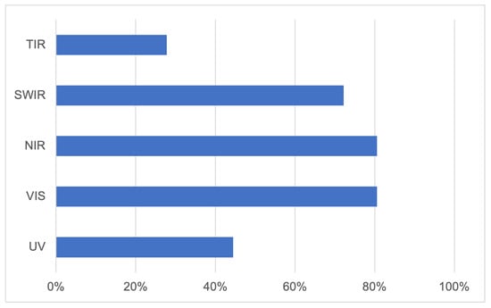
Figure 13. Band frequency use by researchers.

In the latest satellites sent into space (Sentinel program), the temporal resolution is highly advanced, with revisit times between two and six days, allowing frequent and updated monitoring of the same area [81]. Despite this source of temporal data, only four authors carried out temporal analyses [43,50,62,67].

3.1.4. AI Models (EQ 7, EQ8, and EQ9)

Table 3 presents the most commonly used models in the review articles. Most authors found better results for the DL and TNN models (shown by an asterisk in the first column). Deep Neural Networks (DNNs) and Convolutional Neural Networks (CNNs), as well as their derivatives, are the most widely used DL models. Although CNN is a modification of DNN, it was differentiated in Table 3 to maintain the terminology defined by the authors of the selected articles. For TNN, the most used were Artificial Neural Networks (ANNs) and Multi-Layer Perceptron (MLP). Despite the MLP being an ANN, they appear with their own nomenclature to maintain the terminology used by the authors. Random Forest (RF) and Partial Least Squares Regression (PLS) were the most used algorithms for O-ML.

Table 3. Models used to estimate SOC and the most efficient between them.

References	DL	TNN	O-ML	The Most Efficient (${\mathit{R}}^2$)
Odebiri et al. [46]	CAE-DNN DNN Boruta-DNN	Not used	Not used	CAE-DNN
Odebiri et al. [47]	DNN	Not used	Not used	Not applicable
Odebiri et al. [48]	DNN	ANN	RF SVM	DNN
Ma et al. [75]	LeNet-7-CNN 1D LeNet-5	Not used	RF SVM	LeNet-7-CNN
Chang et al. [41]	Not used	BPNN DPSO-BPNN	PLS MSR	DPSO-BPNN
* Zeraatpisheh et al. [53]	Not used	ANN	RF KNN SVM Models ensemble	RF
* Xu et al. [57]	CNN	Not used	SVM PLS LR	PLS
L. Zhang et al. [62]	CNN-LSTM	Not used	RF	CNN-LSTM
* Abdoli et al. [71]	Not used	MLP	SVR GEP	SVR
* Zolfaghari Nia et al. [58]	Not used	ANN	RF KNN RTC CART	RTC
Liu et al. [51]	DNN	MLP	PLS	DNN
Meng et al. [50]	CNN	Not used	RF PLS	CNN
S. Wang et al. [45]	CNN LSTM	ANN	RF PLS Ridge	LSTM
* Fathizad et al. [67]	Not used	MLP	RF SVR	RF
* K. Wang et al. [68]	Not used	ANN	RF SVM PLS	RF
Li et al. [73]	Not used	MLP	Not used	Not applicable
Zeng et al. [76]	LSM-RESNET	Not used	RF	LSM-RESNET
Y. Zhang et al. [59]	SA-DNN	Not used	RF SVM PLS XGB ELM	SA-DNN
F. Zhang et al. [44]	1D-CNN	Not used	PLS	1D-CNN
Li et al. [54]	Not used	ANN	Not used	Not Applicable
Shi et al. [42]	Not used	ANN	RF SVM PLS	ANN
Guo et al. [61]	DNN	Not used	RF	DNN
Bouasria et al. [72]	Not used	MLP	MLR	MLP
X. Wang et al. [52]	Not used	ANN	PLS SVM	ANN
Taghizadeh-Mehrjardi et al. [69]	DNN	ANN	RF SVR GP LAS Lasso KNN ANFIS XGB	ANN
Gadal et al. [43]	Not used	MLP	SVM SAM Parallelepiped MD ML MaD	MLP
* Pellikka et al. [60]	CNN	Not used	RF PLS Lasso GPR	Lasso
* Mallik et al. [63]	Not used	ANN ANN-OK ANN-CK	EBKR	EBKR
Ou et al. [65]	Semi-DNNR	Not used	SVR PLS	Semi-DNNR
* Yang et al. [49]	Not used	ANN	RF PLS SVM	RF
* Budak et al. [64]	Not used	MLP	GBDT	GBDT
* Morais et al. [55]	Not used	ANN	RF MLR XGB	XGB
Samarinas et al. [74]	CNN	Not used	RF PLS SVM Cubist	CNN
* Salani et al. [66]	Not used	MLP	OLS	OLS
Hosseini et al. [70]	CNN RNN Hybrid CNN-RNN	Not used	Not used	Hybrid CNN-RNN
Zayani et al. [56]	DNN	Not used	RF PLS	DNN

Notes: * represents the authors who found better results for O-ML. Recurrent Neural Network (RNN); Long Short-Term Memory (LSTM); Concrete Autoencoder– Deep Neural Network (CAE-DNN); Hybrid Convolutional Neural Network–Recurrent Neural Network (Hybrid CNN-RNN); 1D–Convolutional Neural Network (1D-CNN); Back Propagation Neural Network (BPNN); Dynamic Particle Swarm Optimization–Back Propagation Neural Network (DPSO-BPNN); Simulated Aneling–Deep Neural Network (SA-DNN); Artificial Neural Network–Ordinary Kriging (ANN-OK); Artificial Neural Network–Cokriging (ANN-CK); Semi-Deep Neural Network Regression (Semi-DNNR); Support Vector Machine (SVM); Multiple Stepwise Regression (MSR); K-Nearest Neighbors (KNN); Support Vector Regression (SVR); Genetic Expression Programming (GEP); Lightweight Deep Learning Architecture–Residual Network (LSM-ResNet); 1D LeNet-5–Convolutional Neural Network (1D LeNet-5-CNN); LeNet-7–Convolutional Neural Network (LeNet-7-CNN); Boruta–Convolutional Neural Network (Boruta-CNN); eXtreme Gradient Boosting (XGB); Multiple Linear Regression (MLR); Ordinary Least-Squares (OLS); Gradient Boosted Decision Trees (GBDT); Extreme Learning Machine (ELM); Gaussian Process Regression (GPR); Empirical Bayesian Kriging Regression (EBKR); Spectral Angle Mapper (SAM); Minimum Distance (MD); Mahalanobis Distance (MaD); Adaptive Network-based Fuzzy Inference System (ANFIS); Genetic Programming (GP); Regression tree cubist (Cubist).

Some authors, such as Taghizadeh-Mehrjardi et al. [69], used specific models, called “other averaging methods”, as shown in Table 3, including Akaike’s information criterion, equal weights averaging, Bates–Granger averaging, Bayes’ information criterion, Mallow’s model averaging, Granger–Ramanathan averaging, and Bayesian model averaging.

Figure 14 shows that the DL models demonstrate greater strength in predicting the SOC, with a higher mean and median value in coefficient of determination ($R^2$), indicating greater consistency in the SOC results. In contrast, O-ML models have the lowest median and greatest dispersion of results, indicating less precision and more variability in results. TNN models, on the other hand, have the lowest dispersion among the three, indicating lower variability and, therefore, greater predictive capacity of the SOC.

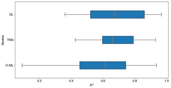
Figure 14. Comparative performance of models through the $R^2$ (The orange line represents the median of the data).

4. Discussion

The interest in this knowledge area is evident when, for 2022, the number of papers is almost triple compared to 2021, and it was almost the same in 2023. The global distribution of articles was similar to that found by Odebiri et al. [17], probably because the same research groups continue to work on the topic in the same countries.

4.1. Study Area and SOC Samples

The use of sampling densities lower than one soil sample per km² in most articles, as shown in Figure 4, is probably related to the high economic cost, labor, and time required for the collection and laboratory analysis of soil samples.

As prediction models, especially DL, depend on a significant volume of data to extract terrain information, the limitation in the number of samples impacts the performance of these algorithms [46,47,48,57,60].

However, L. Zhang et al. [62], Liu et al. [51], and Ou et al. [65] found results, in terms of $R^2$, for DL models greater than TNN or O-ML models, even using a reduced dataset (308, 45, and 95 samples, respectively), although the authors recognize that a more significant number of samples could further improve the performance of DL models.

Almost 70% of the studies considered in this review focus on sampling densities of up to one sample per km², which was considered in this study as low density [43,45,46,47,48,49,62,63,64,65,66,67,68,70,71,72,73,74,75,76].

Figure 15 shows the $R^2$ of the different AI models tested by the authors. The horizontal axis represents the sampling density on a logarithmic scale (LOG10), while the vertical axis shows the $R^2$. The cross indicates the $R^2$ value for the conventional AI model, the red square for the DL model, and the blue square for the TNN model. Thus, for the same database, the authors test the performance of the different AI algorithms, finding that several models can achieve satisfactory or significant $R^2$ values.

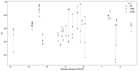
Figure 15. Efficiency of ML models as a function of sampling density.

It is observed that, in general, for lower sampling densities (on the left of the graph), there is greater variability in the efficiency of the models. As the sampling density increases (on the right), the $R^2$ values tend to increase, suggesting that a more significant amount of sample data improves the performance of the models, although there are variations between them. For example, the O-ML models show greater variability in efficiency across all densities, while the DL and TNN models are more consistent in certain regions. At intermediate sampling densities (close to −1 and 1), the DL model reaches high peaks of $R^2$. Nonetheless, the $R^2$ improves with the DL models, and its performance remains high, even for low sample densities, outperforming the other models. These results reinforce the efficiency of these models when working with limited datasets [45,48,65,72,75].

Although DL models can use reduced datasets, the samples must represent the greatest spatial heterogeneity so that the maximum variability is captured and considered by predictive AI models [51]. The spatial distribution of data must be carefully planned to encompass spatial variability. For example, Odebiri et al. [46] and Taghizadeh-Mehrjardi et al. [69] show that high altitude and high humidity increase SOC levels. If these zones are not adequately considered, this can significantly impact the results of the AI model. The spatial distribution refers to the irregularities/roughnesses of the terrain surface, given that SOC predictions with RS refer only to surface soil samples and quickly lose accuracy for deeper soil layers, making it impossible to include soil samples in high depth [73].

Applying a statistical analysis to a bibliographic data matrix (p-value equal to 0.000), it was observed that the sampling density variable explains 36% of the variability in the $R^2$ of the models, with the remaining 64% explained by the other features (e.g., topographic indices, vegetation and soil indices, climate data, among others).

4.2. Input Data

The quality and variability of the input data determine the AI model’s predictive capacity to recognize patterns in the study area. The strength of input data is fundamental to ensure that the data predicted by the AI model is consistent with reality (high predictive capacity), especially in the study areas with significant spatial heterogeneity [54,69].

As reported in the above section and compared to the review by Odebiri et al. [17], a noticeable change can be observed in the data acquisition platforms. On the one hand, satellite data barely represented 35% of the data and are currently used in 80% of review articles. On the other hand, the use of expensive/tedious field spectrophotometers decreases from 48% to 19%. These changes in data acquisition platforms have occurred since 2018, so they can be attributed to the initial use of satellite data from recent Sentinel-2 and Landsat programs, which offer a better spatial, spectral, and temporal resolution than the above satellite data [43,46,47,48,49,50,51,52,53,54,55,56,58,61,63,64,67,68,69,70,71,72,74,75,82].

Vegetation indices obtained from spectral bands (such as NDVI, EVI, SAVI, and others) as input data in AI models are widely used for SOC prediction and correspond to 67% of the review studies. This wide use could be due to the strong influence of the visible/infrared reflectance ratio on the bare soil signal and, consequently, on SOC determination [71,73]. Between many spectral indices, NDVI is one of the most correlated with SOC in models [46,47,48,54,56,57,64,67,69,71,73,75]. Other indices, such as SAVI, RVI, and EVI, also stand out among the best input data in the models [46,47,48,49,54,58,69,71].

According to L. Zhang et al. [62], topographic indices strongly correlate with SOC. These spectral indices, which can differentiate vegetation types (e.g., gymnosperms, angiosperms) or measure biomass/leaf area index, may indirectly provide information about topography [47]. Several studies have used vegetation and topographic indices as model inputs, but there is disagreement regarding which indices have the highest correlation with SOC [43,46,50,53,54,55,57,58,62,63,69,70,73,76]. Although Li et al. [73] compared the combined use of vegetation and topography data, demonstrating better results with data fusion than with topography alone, it is still necessary to investigate both datasets separately to determine which offers the best performance because using too many features can degrade model performance, especially when redundancies exist in the data [46,48,54,71,75].

In addition to spectral data on the surface of the Earth, other environmental variables, such as annual median temperature and rainfall, directly influence SOC content [46,62,69,70]. These climate factors play a crucial role in soil carbon dynamics, affecting processes such as evapotranspiration, organic matter decomposition, and microbial activity, which are essential in the soil C biogeochemical cycle.

4.3. Satellite and Imagery Resolution

Concerning satellites, Sentinel-2 and Landsat 8 were the most used, probably due to the improvement in spatial and spectral resolution compared to previous missions and their open data being easily accessible [17,49]. According to K. Wang et al. [68], Sentinel-2, due to its excellent capacity for inverting soil properties, may be superior to Landsat. MODIS satellite images are also available free of charge; however, they have limitations in their resolutions. Meng et al. and K. Wang et al. [50,68] used data from Chinese Gaofen satellites, but images with good resolutions are provided by private companies, which makes their use more costly.

Spatial resolution is essential in modeling soil characteristics since soil is a complex system influenced by several environmental factors that act at different scales [62]. Higher spatial resolution (i.e., smaller pixel size) provides a greater detail of surface land, allowing spatial variability to be captured with greater accuracy. As evidenced by Odebiri et al. [47], a resolution of 300 m may be sufficient for modeling large areas, showing that models can perform well on national scales with lower resolutions. Currently, compared to the review by Odebiri et al. [17], there is a significant increase in the use of spatial resolutions between 10 and 30 m and a decrease in the use of highly detailed resolutions (<10 m), reflecting the replacement of field spectrophotometers by satellite data. Although obtaining higher-resolution data could improve AI model accuracy, intermediate resolutions offer a good balance between the necessary effort in obtaining data and its strength predictive for large areas.

Regarding the use of multispectral and hyperspectral data, according to Meng et al. [50], the numerous bands and narrower bandwidths of a hyperspectral image allow for better exploration of the spectral features corresponding to the SOC content relative to multispectral images. In his work, the SOC estimations were better from the hyperspectral satellite (GF-5) than those obtained from the Landsat 8 satellite. Liu et al. [51] found similar results using hyperspectral data from the field spectrophotometer (ASD FieldSpec3 sensor) and Headwall Micro-hyperpec, transported by helicopter, compared with Sentinel-2 multispectral data. Xu et al. [57] also found better results for estimating SOC using hyperspectral data. However, other authors argue that using multispectral images is also recurrent, as these are more easily acquired and present promising results [75]. The author also found that the NIR region (783–865 nm) and visible RGB bands (740 nm, 660 nm, and 560 nm) are the most sensitive to SOC variations.

Regarding temporal resolution, according to Dou et al. [83], there is little variability in up to 10 years when the landscape is not drastically changed, which suggests that it is possible to analyze data from different years using a single field sample. Meng et al. [50] found SOC modeling results better when using multitemporal analysis from several satellite images in the same region, with RMSE decreasing and $R^2$ increasing, using a DL model (CNN). Other authors also found better results for multitemporal analyses, which indicates that this little-used technique has great potential [43,62,67].

A practice being explored is using samples at different times and the data corresponding to each period. This approach can provide models with information about how temporal changes are associated with variations in SOC stocks. By integrating temporally varying data, models could identify which inputs contributed to SOC changes over time, enabling the analysis of soil dynamics and improving the models’ ability to detect and quantify environmental and land use influences. With this information, in addition to improving predictions, the models could indicate which variables have the most significant impact on the SOC dynamics.

4.4. AI Models

It is essential to compare the effectiveness of DL, NN, and O-ML models. Although most articles reviewed compare these algorithms to determine the most effective (Table 3), some still need to perform this comparison, using only one or two of these categories for modeling.

The NN and DL techniques proved to be superior in terms of $R^2$ in most of the articles considered in this review, proving to be more robust solutions for SOC estimation [41,42,43,44,45,48,50,51,52,56,59,61,62,65,69,70,72,74,75,76]. In the specific case of DL models, these were rarely surpassed by O-ML or TNN, occurring in only three cases [57,60,69].

Although most DL models used in these studies are not very complex, some are worth explaining in more detail.

Odebiri et al. [46] developed a Concrete Autoencoder–Deep neural network (CAE-DNN), which was revealed to be better in SOC retrieval than a regular DNN and a Boruta-DNN. Their framework starts by eliminating redundant variables and selecting variables using Concrete Autoencoders, and then a DNN is used for the SOC prediction process. The CAE is unsupervised and capable of identifying informative features while reconstructing input data from those selected features because it uses a concrete selector layer as the encoder and a standard NN as the decoder [84]; this is important in estimating SOC, as soil properties are influenced by many variables that are not equally relevant for prediction. A gradual decrease in temperature in the concrete selector layer during training encourages learning a user-specified number of discrete features. During testing, the selected features can be used to reconstruct the remaining input features using the decoder network. Concrete autoencoders are simple to set up and scale well to large datasets, making them a versatile and useful tool for feature selection and data reduction. This model type is an innovation in SOC data recovery, as Odebiri et al. [17] reported in their review. This type of algorithm has yet to be used previously and could be used for SOC prediction, as they were adequate for other similar tasks. Moreover, L. Zhang et al. [62] developed a CNN-LSTM to handle both spatial and temporal information in data. It begins by employing a CNN to extract spatial features from climate and terrain variables, which are commonly related to SOC, effectively converting them to image-like data. Following that, a Long Short-Term Memory (LSTM) network is used to extract temporal features from phenological and EVI time series data, which are also data related to SOC. These spatial and temporal features are concatenated and processed through fully connected layers to predict SOC content. The model’s ability to handle various environmental covariates and extract contextual information in both spatial and temporal domains make it a promising tool for Digital Soil Mapping (DSM) tasks, including SOC mapping, even with limited soil sample data.

Y. Zhang et al. [59] used hyperspectral imagery to map the available copper (ACu) content in the soil using a Simulated Annealing Deep Neural Network (SA-DNN). The SA-DNN method selects relevant spectral bands by combining hyperspectral data with Competitive Adaptive Reweighted Sampling (CARS) and modeling with a DNN architecture enhanced with simulated annealing. The model’s performance was evaluated, demonstrating high accuracy in predicting ACu and SOM content. This method showed the efficacy of using UAV hyperspectral imagery with SA-DNN for soil environmental monitoring and mapping.

Most studies that show a higher accuracy rate in SOC estimation prediction using O-ML methods only compared these traditional models with TNN methods [49,53,58,64,67,68,71]. Only two studies reported in this review presented better results using O-ML than using DL techniques [57,60]. Moreover, both agreed that the DL models used in their research were not very effective due to the lack of training data.

5. Conclusions

This review demonstrates that DL models consistently outperform TNNs and other machine-learning models and that, contrary to initial assumptions, using a large number of SOC data is unnecessary to achieve good model performance. After analyzing more than 60 papers, it became evident that the samples’ spatial distribution and variability are more critical than the total number of samples.

Spectral indices such as NDVI, SAVI, and EVI, along with topographic indices obtained from DEMs, were identified as the most influential inputs for SOC prediction. Due to their improved resolutions, the Sentinel-2 and Landsat 8 satellites were the main data sources.

Although DL methods present greater robustness and predictive power than others identified in this literature review, challenges such as limited data availability and possible redundancy of input variables persist. Future research should focus on improving variable selection processes and exploring integrating multitemporal and hyperspectral data to improve model performance. This study reaffirms the potential of RS and advanced computational techniques in monitoring SOC, allowing the collection of information quickly, cheaply, and without harm to the environment.

References

- Millennium Ecosystem Assessment. Ecosystems and Human Well-Being: Desertification Synthesis; World Resources Institute: Washington, DC, USA, 2005. [Google Scholar]
- Bronick, C.J.; Lal, R. Soil structure and management: A review. Geoderma 2005, 124, 3–22. [Google Scholar] [CrossRef]
- Pribyl, D.W. A critical review of the conventional SOC to SOM conversion factor. Geoderma 2010, 156, 75–83. [Google Scholar] [CrossRef]
- Obour, P.B.; Jensen, J.L.; Lamandé, M.; Watts, C.W.; Munkholm, L.J. Soil organic matter widens the range of water contents for tillage. Soil Tillage Res. 2018, 182, 57–65. [Google Scholar] [CrossRef] [PubMed]
- Shukla, M.; Lal, R.; Ebinger, M. Determining soil quality indicators by factor analysis. Soil Tillage Res. 2006, 87, 194–204. [Google Scholar] [CrossRef]
- Lorenz, K.; Lal, R.; Ehlers, K. Soil organic carbon stock as an indicator for monitoring land and soil degradation in relation to United N ations’ Sustainable Development eoals. Land Degrad. Dev. 2019, 30, 824–838. [Google Scholar] [CrossRef]
- Poeplau, C. Measuring and Modelling Soil Carbon Stocks and Stock Changes in Livestock Production Systems: Guidelines for Assessment; Version 1—Advanced Copy; Johann Heinrich von Thünen-Institut: Braunschweig, Germany, 2019. [Google Scholar]
- Peralta, G.; Di Paolo, L.; Luotto, I.; Omuto, C.; Mainka, M.; Viatkin, K.; Yigini, Y. Global Soil Organic Carbon Sequestration Potential Map (GSOCseq v1. 1)—Technical Manual; Food & Agriculture Org.: Rome, Italy, 2022. [Google Scholar]
- Agjee, N.; Mutanga, O.; Ismail, R. Remote sensing bio-control damage on aquatic invasive alien plant species. S. Afr. J. Geomat. 2015, 4, 464–485. [Google Scholar] [CrossRef][Green Version]
- Odindi, J.; Bangamwabo, V.; Mutanga, O. Assessing theValue ofUrbanGreen Spaces inMitigatingMulti-SeasonalUrban Heat using MODISLand SurfaceTemperature (LST) and Landsat 8 data. Int. J. Environ. Res. 2015, 9, 9–18. [Google Scholar]
- Walkley, A.; Black, I.A. An examination of the Degtjareff method for determining soil organic matter, and a proposed modification of the chromic acid titration method. Soil Sci. 1934, 37, 29–38. [Google Scholar] [CrossRef]
- Nelson, D.W.; Sommers, L.E. Total carbon, organic carbon, and organic matter. Methods Soil Anal. Part 3 Chem. Methods 1996, 5, 961–1010. [Google Scholar]
- Li, S.; Viscarra Rossel, R.A.; Webster, R. The cost-effectiveness of reflectance spectroscopy for estimating soil organic carbon. Eur. J. Soil Sci. 2022, 73, e13202. [Google Scholar] [CrossRef]
- Rossel, R.V.; Behrens, T. Using data mining to model and interpret soil diffuse reflectance spectra. Geoderma 2010, 158, 46–54. [Google Scholar] [CrossRef]
- Rossel, R.V.; Walvoort, D.; McBratney, A.; Janik, L.J.; Skjemstad, J. Visible, near infrared, mid infrared or combined diffuse reflectance spectroscopy for simultaneous assessment of various soil properties. Geoderma 2006, 131, 59–75. [Google Scholar] [CrossRef]
- Gomez, C.; Rossel, R.A.V.; McBratney, A.B. Soil organic carbon prediction by hyperspectral remote sensing and field vis-NIR spectroscopy: An Australian case study. Geoderma 2008, 146, 403–411. [Google Scholar] [CrossRef]
- Odebiri, O.; Mutanga, O.; Odindi, J.; Naicker, R.; Masemola, C.; Sibanda, M. Deep learning approaches in remote sensing of soil organic carbon: A review of utility, challenges, and prospects. Environ. Monit. Assess. 2021, 193, 1–18. [Google Scholar] [CrossRef]
- Mngadi, M.; Odindi, J.; Peerbhay, K.; Mutanga, O. Examining the effectiveness of Sentinel-1 and 2 imagery for commercial forest species mapping. Geocarto Int. 2021, 36, 1–12. [Google Scholar] [CrossRef]
- Khanal, S.; Fulton, J.; Klopfenstein, A.; Douridas, N.; Shearer, S. Integration of high resolution remotely sensed data and machine learning techniques for spatial prediction of soil properties and corn yield. Comput. Electron. Agric. 2018, 153, 213–225. [Google Scholar] [CrossRef]
- Odebiri, O.; Mutanga, O.; Odindi, J.; Peerbhay, K.; Dovey, S.; Ismail, R. Estimating soil organic carbon stocks under commercial forestry using topo-climate variables in KwaZulu-Natal, South Africa. S. Afr. J. Sci. 2020, 116, 1–8. [Google Scholar] [CrossRef]
- Hamida, A.B.; Benoit, A.; Lambert, P.; Amar, C.B. 3-D deep learning approach for remote sensing image classification. IEEE Trans. Geosci. Remote Sens. 2018, 56, 4420–4434. [Google Scholar] [CrossRef]
- Pudełko, A.; Chodak, M. Estimation of total nitrogen and organic carbon contents in mine soils with NIR reflectance spectroscopy and various chemometric methods. Geoderma 2020, 368, 114306. [Google Scholar] [CrossRef]
- Madileng, N.P.; Mutanga, O.; Dube, T.; Odebiri, O. Mapping the spatial distribution of Lantana camara using high-resolution SPOT 6 data, in Mpumalanga communal areas, South Africa. Trans. R. Soc. S. Afr. 2020, 75, 239–244. [Google Scholar] [CrossRef]
- Padarian, J.; Minasny, B.; McBratney, A. Transfer learning to localise a continental soil vis-NIR calibration model. Geoderma 2019, 340, 279–288. [Google Scholar] [CrossRef]
- Mouazen, A.; Kuang, B.; De Baerdemaeker, J.; Ramon, H. Comparison among principal component, partial least squares and back propagation neural network analyses for accuracy of measurement of selected soil properties with visible and near infrared spectroscopy. Geoderma 2010, 158, 23–31. [Google Scholar] [CrossRef]
- Jaber, S.M.; Lant, C.L.; Al-Qinna, M.I. Estimating spatial variations in soil organic carbon using satellite hyperspectral data and map algebra. Int. J. Remote Sens. 2011, 32, 5077–5103. [Google Scholar] [CrossRef]
- Li, Q.Q.; Zhang, X.; Wang, C.Q.; Li, B.; Gao, X.S.; Yuan, D.G.; Luo, Y.L. Spatial prediction of soil nutrient in a hilly area using artificial neural network model combined with kriging. Arch. Agron. Soil Sci. 2016, 62, 1541–1553. [Google Scholar] [CrossRef]
- Yuan, Q.; Shen, H.; Li, T.; Li, Z.; Li, S.; Jiang, Y.; Xu, H.; Tan, W.; Yang, Q.; Wang, J.; et al. Deep learning in environmental remote sensing: Achievements and challenges. Remote Sens. Environ. 2020, 241, 111716. [Google Scholar] [CrossRef]
- Huang, G.B.; Zhu, Q.Y.; Siew, C.K. Extreme learning machine: A new learning scheme of feedforward neural networks. In Proceedings of the 2004 IEEE International Joint Conference on Neural Networks (IEEE Cat. No. 04CH37541), Budapest, Hungary, 25–29 July 2004; Volume 2, pp. 985–990. [Google Scholar]
- Ma, L.; Liu, Y.; Zhang, X.; Ye, Y.; Yin, G.; Johnson, B.A. Deep learning in remote sensing applications: A meta-analysis and review. ISPRS J. Photogramm. Remote Sens. 2019, 152, 166–177. [Google Scholar] [CrossRef]
- Odebiri, O.; Odindi, J.; Mutanga, O. Basic and deep learning models in remote sensing of soil organic carbon estimation: A brief review. Int. J. Appl. Earth Obs. Geoinf. 2021, 102, 102389. [Google Scholar] [CrossRef]
- Kitchenham, B.; Charters, S. Guidelines for performing Systematic Literature Reviews in Software Engineering, 2007. Available online: https://www.researchgate.net/profile/Barbara-Kitchenham/publication/302924724_Guidelines_for_performing_Systematic_Literature_Reviews_in_Software_Engineering/links/61712932766c4a211c03a6f7/Guidelines-for-performing-Systematic-Literature-Reviews-in-Software-Engineering.pdf (accessed on 10 July 2024).
- Brancalião, L.; Gonçalves, J.; Conde, M.Á.; Costa, P. Systematic Mapping Literature Review of Mobile Robotics Competitions. Sensors 2022, 22, 2160. [Google Scholar] [CrossRef]
- Kitchenham, B.; Brereton, O.P.; Budgen, D.; Turner, M.; Bailey, J.; Linkman, S. Systematic literature reviews in software engineering–a systematic literature review. Inf. Softw. Technol. 2009, 51, 7–15. [Google Scholar] [CrossRef]
- Kitchenham, B. Procedures for Performing Systematic Reviews; (Keele University Technical Report No. TR/SE-0401; NICTA Technical Report No. 0400011T. 1); Keele University: Keele, UK, 2004. [Google Scholar]
- Camargo, C.; Gonçalves, J.; Conde, M.Á.; Rodríguez-Sedano, F.J.; Costa, P.; García-Peñalvo, F.J. Systematic Literature Review of Realistic Simulators Applied in Educational Robotics Context. Sensors 2021, 21, 4031. [Google Scholar] [CrossRef]
- Higgins, J.P.D.; Altman, D.G.; Sterne, J.A.C. (Eds.) Chapter 8: Assessing risk of bias in included studies. In: Higgins JPT, Churchill R, Chandler J, Cumpston MS (editors). Cochrane Handbook for Systematic Reviews of Interventions. version 5.2.0 (updated June 2017), Cochrane, 2017. Available online: https://training.cochrane.org/sites/training.cochrane.org/files/public/uploads/resources/Handbook5_1/Chapter_8_Handbook_5_2_8.pdf (accessed on 10 July 2024).
- Popay, J.; Roberts, H.; Sowden, A.; Petticrew, M.; Arai, L.; Rodgers, M.; Britten, N.; Roen, K.; Duffy, S. Guidance on the conduct of narrative synthesis in systematic reviews. In A Product from the ESRC Methods Programme Version; Lancaster University: Lancaster, UK, 2006; Volume 1, p. b92. [Google Scholar]
- Cruz-Benito, J. Systematic Literature Review & Mapping. 2016. Available online: https://repositorio.grial.eu/server/api/core/bitstreams/2806d401-914e-4524-97b7-c7ef859908d1/content (accessed on 10 July 2024).
- Page, M.J.; McKenzie, J.E.; Bossuyt, P.M.; Boutron, I.; Hoffmann, T.C.; Mulrow, C.D.; Shamseer, L.; Tetzlaff, J.M.; Akl, E.A.; Brennan, S.E.; et al. The PRISMA 2020 statement: An updated guideline for reporting systematic reviews. BMJ 2021, 372, n71. [Google Scholar] [CrossRef] [PubMed]
- Chang, R.; Chen, Z.; Wang, D.; Guo, K. Hyperspectral Remote Sensing Inversion and Monitoring of Organic Matter in Black Soil Based on Dynamic Fitness Inertia Weight Particle Swarm Optimization Neural Network. Remote Sens. 2022, 14, 4316. [Google Scholar] [CrossRef]
- Shi, Y.; Zhao, J.; Song, X.; Qin, Z.; Wu, L.; Wang, H.; Tang, J. Hyperspectral band selection and modeling of soil organic matter content in a forest using the Ranger algorithm. PLoS ONE 2021, 16, e0253385. [Google Scholar] [CrossRef] [PubMed]
- Gadal, S.; Oukhattar, M.; Keller, C.; Hanadé, I. Spatio-temporal modelling of relationship between Organic Carbon Content and Land Use using Deep Learning approach and several covariables: Application to the soils of the Beni Mellal in Morocco. In Proceedings of the GISTAM 2023 9th International Conference on Geographical Information Systems Theory, Applications and Management, SCITEPRESS, Prague, Czech Republic, 25–27 April 2023; Volume 1, pp. 15–26. [Google Scholar]
- Zhang, F.; Wang, C.; Pan, K.; Guo, Z.; Liu, J.; Xu, A.; Ma, H.; Pan, X. The Simultaneous Prediction of Soil Properties and Vegetation Coverage from Vis-NIR Hyperspectral Data with a One-Dimensional Convolutional Neural Network: A Laboratory Simulation Study. Remote Sens. 2022, 14, 397. [Google Scholar] [CrossRef]
- Wang, S.; Guan, K.; Zhang, C.; Lee, D.; Margenot, A.J.; Ge, Y.; Peng, J.; Zhou, W.; Zhou, Q.; Huang, Y. Using soil library hyperspectral reflectance and machine learning to predict soil organic carbon: Assessing potential of airborne and spaceborne optical soil sensing. Remote Sens. Environ. 2022, 271, 112914. [Google Scholar] [CrossRef]
- Odebiri, O.; Mutanga, O.; Odindi, J.; Naicker, R. Mapping soil organic carbon distribution across South Africa’s major biomes using remote sensing-topo-climatic covariates and Concrete Autoencoder-Deep neural networks. Sci. Total. Environ. 2023, 865, 161150. [Google Scholar] [CrossRef]
- Odebiri, O.; Mutanga, O.; Odindi, J.; Naicker, R. Modelling soil organic carbon stock distribution across different land-uses in South Africa: A remote sensing and deep learning approach. ISPRS J. Photogramm. Remote Sens. 2022, 188, 351–362. [Google Scholar] [CrossRef]
- Odebiri, O.; Mutanga, O.; Odindi, J. Deep learning-based national scale soil organic carbon mapping with Sentinel-3 data. Geoderma 2022, 411, 115695. [Google Scholar] [CrossRef]
- Yang, J.; Fan, J.; Lan, Z.; Mu, X.; Wu, Y.; Xin, Z.; Miping, P.; Zhao, G. Improved Surface Soil Organic Carbon Mapping of SoilGrids250m Using Sentinel-2 Spectral Images in the Qinghai–Tibetan Plateau. Remote Sens. 2022, 15, 114. [Google Scholar] [CrossRef]
- Meng, X.; Bao, Y.; Wang, Y.; Zhang, X.; Liu, H. An advanced soil organic carbon content prediction model via fused temporal-spatial-spectral (TSS) information based on machine learning and deep learning algorithms. Remote Sens. Environ. 2022, 280, 113166. [Google Scholar] [CrossRef]
- Liu, Q.; He, L.; Guo, L.; Wang, M.; Deng, D.; Lv, P.; Wang, R.; Jia, Z.; Hu, Z.; Wu, G.; et al. Digital mapping of soil organic carbon density using newly developed bare soil spectral indices and deep neural network. Catena 2022, 219, 106603. [Google Scholar] [CrossRef]
- Wang, X.; Han, J.; Wang, X.; Yao, H.; Zhang, L. Estimating soil organic matter content using sentinel-2 imagery by machine learning in shanghai. IEEE Access 2021, 9, 78215–78225. [Google Scholar] [CrossRef]
- Zeraatpisheh, M.; Ayoubi, S.; Mirbagheri, Z.; Mosaddeghi, M.R.; Xu, M. Spatial prediction of soil aggregate stability and soil organic carbon in aggregate fractions using machine learning algorithms and environmental variables. Geoderma Reg. 2021, 27, e00440. [Google Scholar] [CrossRef]
- Li, Y.; Zhang, Z.; Zhao, Z.; Sun, D.; Zhu, H.; Zhang, G.; Zhu, X.; Ding, X. Zoning Prediction and Mapping of Three-Dimensional Forest Soil Organic Carbon: A Case Study of Subtropical Forests in Southern China. Forests 2023, 14, 1197. [Google Scholar] [CrossRef]
- Morais, T.G.; Jongen, M.; Tufik, C.; Rodrigues, N.R.; Gama, I.; Serrano, J.; Gonçalves, M.C.; Mano, R.; Domingos, T.; Teixeira, R.F. Satellite-based estimation of soil organic carbon in Portuguese grasslands. Front. Environ. Sci. 2023, 11, 1240106. [Google Scholar] [CrossRef]
- Zayani, H.; Fouad, Y.; Michot, D.; Kassouk, Z.; Baghdadi, N.; Vaudour, E.; Lili-Chabaane, Z.; Walter, C. Using Machine-Learning Algorithms to Predict Soil Organic Carbon Content from Combined Remote Sensing Imagery and Laboratory Vis-NIR Spectral Datasets. Remote Sens. 2023, 15, 4264. [Google Scholar] [CrossRef]
- Xu, X.; Du, C.; Ma, F.; Qiu, Z.; Zhou, J. A framework for high-resolution mapping of soil organic matter (SOM) by the integration of fourier mid-infrared attenuation total reflectance spectroscopy (FTIR-ATR), sentinel-2 images, and DEM derivatives. Remote Sens. 2023, 15, 1072. [Google Scholar] [CrossRef]
- Zolfaghari Nia, M.; Moradi, M.; Moradi, G.; Taghizadeh-Mehrjardi, R. Machine learning models for prediction of soil properties in the riparian forests. Land 2022, 12, 32. [Google Scholar] [CrossRef]
- Zhang, Y.; Wei, L.; Lu, Q.; Zhong, Y.; Yuan, Z.; Wang, Z.; Li, Z.; Yang, Y. Mapping soil available copper content in the mine tailings pond with combined simulated annealing deep neural network and UAV hyperspectral images. Environ. Pollut. 2023, 320, 120962. [Google Scholar] [CrossRef]
- Pellikka, P.; Luotamo, M.; Sädekoski, N.; Hietanen, J.; Vuorinne, I.; Räsänen, M.; Heiskanen, J.; Siljander, M.; Karhu, K.; Klami, A. Tropical altitudinal gradient soil organic carbon and nitrogen estimation using Specim IQ portable imaging spectrometer. Sci. Total. Environ. 2023, 883, 163677. [Google Scholar] [CrossRef]
- Guo, Z.; Li, Y.; Wang, X.; Gong, X.; Chen, Y.; Cao, W. Remote Sensing of Soil Organic Carbon at Regional Scale Based on Deep Learning: A Case Study of Agro-Pastoral Ecotone in Northern China. Remote Sens. 2023, 15, 3846. [Google Scholar] [CrossRef]
- Zhang, L.; Cai, Y.; Huang, H.; Li, A.; Yang, L.; Zhou, C. A CNN-LSTM model for soil organic carbon content prediction with long time series of MODIS-based phenological variables. Remote Sens. 2022, 14, 4441. [Google Scholar] [CrossRef]
- Mallik, S.; Bhowmik, T.; Mishra, U.; Paul, N. Mapping and prediction of soil organic carbon by an advanced geostatistical technique using remote sensing and terrain data. Geocarto Int. 2022, 37, 2198–2214. [Google Scholar] [CrossRef]
- Budak, M.; Günal, E.; Kılıç, M.; Çelik, İ.; Sırrı, M.; Acir, N. Improvement of spatial estimation for soil organic carbon stocks in Yuksekova plain using Sentinel 2 imagery and gradient descent–boosted regression tree. Environ. Sci. Pollut. Res. 2023, 30, 53253–53274. [Google Scholar] [CrossRef]
- Ou, D.; Tan, K.; Lai, J.; Jia, X.; Wang, X.; Chen, Y.; Li, J. Semi-supervised DNN regression on airborne hyperspectral imagery for improved spatial soil properties prediction. Geoderma 2021, 385, 114875. [Google Scholar] [CrossRef]
- Salani, G.M.; Lissoni, M.; Bianchini, G.; Brombin, V.; Natali, S.; Natali, C. Soil organic carbon estimation in Ferrara (Northern Italy) combining in situ geochemical analyses and hyperspectral remote sensing. Environments 2023, 10, 173. [Google Scholar] [CrossRef]
- Fathizad, H.; Taghizadeh-Mehrjardi, R.; Hakimzadeh Ardakani, M.A.; Zeraatpisheh, M.; Heung, B.; Scholten, T. Spatiotemporal assessment of soil organic carbon change using machine-learning in arid regions. Agronomy 2022, 12, 628. [Google Scholar] [CrossRef]
- Wang, K.; Qi, Y.; Guo, W.; Zhang, J.; Chang, Q. Retrieval and mapping of soil organic carbon using Sentinel-2A spectral images from bare cropland in autumn. Remote Sens. 2021, 13, 1072. [Google Scholar] [CrossRef]
- Taghizadeh-Mehrjardi, R.; Khademi, H.; Khayamim, F.; Zeraatpisheh, M.; Heung, B.; Scholten, T. A comparison of model averaging techniques to predict the spatial distribution of soil properties. Remote Sens. 2022, 14, 472. [Google Scholar] [CrossRef]
- Hosseini, F.S.; Razavi-Termeh, S.V.; Sadeghi-Niaraki, A.; Choi, S.M.; Jamshidi, M. Spatial prediction of physical and chemical properties of soil using optical satellite imagery: A state-of-the-art hybridization of deep learning algorithm. Front. Environ. Sci. 2023, 11, 1279712. [Google Scholar] [CrossRef]
- Abdoli, P.; Khanmirzaei, A.; Hamzeh, S.; Rezaei, S.; Moghimi, S. Use of remote sensing data to predict soil organic carbon in some agricultural soils of Iran. Remote Sens. Appl. Soc. Environ. 2023, 30, 100969. [Google Scholar] [CrossRef]
- Bouasria, A.; Ibno Namr, K.; Rahimi, A.; Ettachfini, E.M.; Rerhou, B. Evaluation of Landsat 8 image pansharpening in estimating soil organic matter using multiple linear regression and artificial neural networks. Geo-Spat. Inf. Sci. 2022, 25, 353–364. [Google Scholar] [CrossRef]
- Li, Y.; Zhao, Z.; Wei, S.; Sun, D.; Yang, Q.; Ding, X. Prediction of regional forest soil nutrients based on Gaofen-1 remote sensing data. Forests 2021, 12, 1430. [Google Scholar] [CrossRef]
- Samarinas, N.; Tsakiridis, N.L.; Kokkas, S.; Kalopesa, E.; Zalidis, G.C. Soil Data Cube and Artificial Intelligence Techniques for Generating National-Scale Topsoil Thematic Maps: A Case Study in Lithuanian Croplands. Remote Sens. 2023, 15, 5304. [Google Scholar] [CrossRef]
- Ma, L.; Zhao, L.; Cao, L.; Li, D.; Chen, G.; Han, Y. Inversion of Soil Organic Matter Content Based on Improved Convolutional Neural Network. Sensors 2022, 22, 7777. [Google Scholar] [CrossRef]
- Zeng, P.; Song, X.; Yang, H.; Wei, N.; Du, L. Digital Soil Mapping of Soil Organic Matter with Deep Learning Algorithms. ISPRS Int. J. Geo-Inf. 2022, 11, 299. [Google Scholar] [CrossRef]
- Pettorelli, N.; Vik, J.O.; Mysterud, A.; Gaillard, J.M.; Tucker, C.J.; Stenseth, N.C. Using the satellite-derived NDVI to assess ecological responses to environmental change. Trends Ecol. Evol. 2005, 20, 503–510. [Google Scholar] [CrossRef]
- Huete, A.; Liu, H.; Batchily, K.; Van Leeuwen, W. A comparison of vegetation indices over a global set of TM images for EOS-MODIS. Remote Sens. Environ. 1997, 59, 440–451. [Google Scholar] [CrossRef]
- Chuvieco, E. Fundamentals of Satellite Remote Sensing: An Environmental Approach; CRC Press: Boca Raton, FL, USA, 2020. [Google Scholar]
- Velastegui-Montoya, A.; Montalván-Burbano, N.; Carrión-Mero, P.; Rivera-Torres, H.; Sadeck, L.; Adami, M. Google Earth Engine: A global analysis and future trends. Remote Sens. 2023, 15, 3675. [Google Scholar] [CrossRef]
- Sentiwiki Copernicus. Available online: https://sentiwiki.copernicus.eu/web/?l=en (accessed on 21 October 2024).
- Tripathi, A.; Tiwari, R.K.; Tiwari, S.P. A deep learning multi-layer perceptron and remote sensing approach for soil health based crop yield estimation. Int. J. Appl. Earth Obs. Geoinf. 2022, 113, 102959. [Google Scholar] [CrossRef]
- Dou, X.; Wang, X.; Liu, H.; Zhang, X.; Meng, L.; Pan, Y.; Yu, Z.; Cui, Y. Prediction of soil organic matter using multi-temporal satellite images in the Songnen Plain, China. Geoderma 2019, 356, 113896. [Google Scholar] [CrossRef]
- Abid, A.; Balin, M.F.; Zou, J. Concrete Autoencoders for Differentiable Feature Selection and Reconstruction. arXiv 2019, arXiv:1901.09346. [Google Scholar]
Disclaimer/Publisher’s Note: The statements, opinions and data contained in all publications are solely those of the individual author(s) and contributor(s) and not of MDPI and/or the editor(s). MDPI and/or the editor(s) disclaim responsibility for any injury to people or property resulting from any ideas, methods, instructions or products referred to in the content. |
© 2025 by the authors. Licensee MDPI, Basel, Switzerland. This article is an open access article distributed under the terms and conditions of the Creative Commons Attribution (CC BY) license (https://creativecommons.org/licenses/by/4.0/).