Multimodal Distribution of Positioning Errors in NRTK GNSS CORSs: A Case Study in Sicily (Italy)

Abstract

In the last 20 years, NRTK GNSS CORS networks have been designed, developed, and employed in Sicily (Italy) for research purposes. Following a comprehensive description of the CORS networks in this region, this study aims to compare results obtained from multiple reference points with known coordinates. The analysis will not only account for the various CORS networks to which these points belong but also examine the different correction streams applied in NRTK surveys. The assumption of a normal distribution, which is often assumed for the positioning errors, is generally confirmed by applying the areal stream corrections (FKP, MAX, iMAX), but still, a multimodal distribution is evident when punctual corrections (Nearest and VRS) are applied. The representation of the results in a GIS environment allows for showing the different patterns for some differential correction streams. A statistical approach allowed confirming the trends of the different distribution frequencies of the residuals of the coordinates and quantifying separately the correlation with parameters involved in the analysis. The correlation retrieved is predominantly weak and very weak for all CORS, except for one of those analyzed, for which the correlation is moderate. The correlation became strong for the same CORS, if all parameters are included, for both planimetric and plano-altimetric components (r = 0.6 and r = 0.7, respectively).

1. Introduction

The Global Navigation Satellite System (GNSS) revolution has made it easier for scientists all over the world to construct infrastructure suitable for wide-ranging Earth monitoring investigations. As is widely known, there are several fully operational satellite navigation systems, such as the Chinese BeiDou Navigation Satellite System (BDS [1]), the European Galileo [2], the Russian GLONASS [3], and the American Navstar GPS [4].

The other three GNSS systems will be available in the next few years, such as those defined as Regional Navigation Satellite Systems (RNSSs), including the Indian Regional Navigation Satellite System (IRNSS/NavIC) [5] or Japanese Quasi-Zenith Satellite System (QZSS [6]) and Regional South Korean Positioning System (KPS) [7].

This represents a massive potential for the scientific community to develop studies that will certainly improve the lives of the world’s population. Indeed, besides historical applications (such as those of Positioning and Orbiting, Meteorology, Ionosphere and Space Weather, Reflectometry, Earthquake Monitoring, Integrated Techniques for Land and Structural Health Monitoring, SHM) and Congruence with Different Modes’ Solutions (Network Real-Time Kinematic, NRTK, Precise Point Positioning, PPP, or Static), GNSS systems will provide exciting applications.

Among the most recent and noteworthy are certainly Autonomous Space Navigation, Atmospheric Modeling, Reflectometry by Remote Sensing (Soil and Moisture Content (SMC), Precision Farming (PF), Earth Remote Sensing from SmallSats) as ocean monitoring, forest and wetland hydrology, and, last but not least, as natural hazards [8].

The impressive volume of data provided by GNSS finds application in hardware and software infrastructures, such as using Continuously Operating Reference Stations (CORSs), which, at different scales (global, regional, and national), allow scientific institutions and professionals to access data free of charge. Moreover, regarding the upcoming CORS upgrades to quad-constellation currently operational (BDS, Galileo, GLONASS, GPS), these infrastructures can provide unlimited potential for both technical and scientific applications, e.g., the evaluation of a global reference system and its inconstancy, geodynamic analysis, mining, surveying and land cadastral management, soil moisture mapping, drought, snow depth, airborne Unmanned Aerial Vehicle (UAV), road and rail transport and logistics, maritime navigation, and aviation.

In other ways, GNNS applications have historically been found in positioning for the analysis of three-dimensional (3D) positioning by using CORS. The scientific and technical applications developed in different parts of the continents involved CORS networks for evaluating 3D positioning in real-time NRTK and in post-process analyses. Indeed, the innovative framework of GNSS CORS networks allowed receiving the most reliable differential corrections over an area by using the virtual reference station (VRS), the Flächen–Korrektur Parameter (FKP), or Multi-Reference Station (MRS) approaches. Many studies were also carried out by applying the multi-GNSS Precise Point Positioning (PPP) technique. As a consequence, the use of CORS networks allowed for increasing the distances between reference stations, contemporarily reducing the total amount of CORS distributed over the same area. Moreover, many advantages have been observed in terms of economic impact and network management.

Upon conducting an in-depth literature review, it is immediately noticeable that the most commonly used differential correction in technical and scientific fields is VRS.

Many authors in the literature have studied the results obtained from the different computing streams of differential corrections: among those that we report in the text, those of Gordini et al. and Heo et al. are undoubtedly significant; in these works, adopting an NRTK VRS approach, centimetric positioning results were obtained [9,10]. Zhang et al. instead, using a dataset of 24 h, discussed how to generate zero difference observations based on the double difference atmospheric delay, to reduce the pseudorange multipath effect on the VRS station; the RTK algorithm was used to obtained 97.6% fixed solution with the RMS of ±1.1 cm in north, ±1.1 cm in east, and ±3.0 cm in up direction [11].

Also, Freeland et al. used VRS correction for PF, with particular attention to agricultural tractor/machine RTK control [12]. VRS correction has historically been employed in many technical and scientific applications; noteworthy are Yu et al., who evaluated the preliminary analysis of positioning performance with BDS VRS technology [13], while Wang et al. recently assessed the network RTK service performance under the new signal system of BDS-3, with horizontal and elevation accuracies within ±1 cm and ±2 cm [14].

Instead, Lambrou and Kanellopoulos investigated a methodology for calibration of a single GNSS receiver and evaluated a new supplement to the ISO rules (the existing ISO 17,123-8 [15], which informs the user only of internal accuracy) using the VRS method [16].

Correspondingly, Zhao et al. studied the application of VRS transmission by NRTK-CORS in Landslide Monitoring [17], while Tusat showed a comparison of the accuracy of VRS and static GPS measurement results for the production of topographic maps and spatial data [18]. In this specific area of research is embedded the paper of Charoenkalunyuta et al. [19], which investigated the horizontal accuracy of GNSS cadastral surveying using the Thai-NRTK GNSS CORS VRS network, after investigating about more of 2100 reference marks, a maximum distance from CORS of 50 km was recommended to obtain reliable positioning for cadastral surveying.

On the other hand, Zhang et al. carried out an experiment on VRS in geological hazard monitoring applications, obtaining results with root mean square (RMS) values of all three directions are ±3.7 mm, ±9.2 mm, and ±5.0 mm, respectively [20]. More recently, Elsobeiey, using a three-hour duration session, assessed the performance of VRS for bathymetry determination, and checked how far these techniques meet the minimum standards of the International Hydrography Organization (IHO). It is shown that the Total Horizontal Uncertainty (THU) and Total Vertical Uncertainty (TVU) of the VRS technique meet the IHO standards for all surveys, with ±5.75 cm and ±7.05 cm, at a 95% confidence level [21].

Less common in technical applications and more widely used in scientific ones is the FKP area correction, such as Park and Kee, who proposed a method that combines compact Real-Time Kinematic (RTK) and reference station (RS) networking techniques such as VRS, FKP, and MRS. Results show a true position with ±6–7 cm horizontal and ±7–8 cm vertical error (95%) in an area of 100 by 100 km [22].

Equally significant is the paper of Gümüş et al., in which using a test network consisting of 56 stations showed that the methods from the most accurate to the least accurate were classical RTK, Net-RTK-VRS, and Net-RTK-FKP. In general, horizontal components were found to be two times better than vertical components, ranging from ±1 mm to approximately ±5 cm [23]. Comparing VRS and FKP solution stream data, Gökdaş and Özlüdemir did not find significant differences between the solutions. The mean differences were at the millimeter level, in their work [24].

These results are also in accordance with Dardanelli et al., in which the NRTK positioning has been obtained with different methods (VRS, FKP, Nearest) and the PPP solution has been calculated with two different software (RTKLIB version 2.4.2 p13and CSRS-PPP version 3.50.0). A statistical approach has been performed to check if the distribution frequencies of the coordinates’ residual belong to the normal distribution, for all pairs analyzed. The results confirm that the hypothesis of a normal distribution holds in most pairs. Specifically, the Static vs. NRTK pair appears to achieve the best congruence while using the PPP approach. Notably, pairs obtained with CSRS software exhibit better congruence than those involving RTKLIB software [25].

In contrast to the work of Öğütcü and Kalayci, the TUSAGA-Aktif CORS network was used to obtain the three NRTK corrections (VRS, FKP, MRS). In terms of accuracy, results showed that all the techniques are practically the same, and the horizontal positioning accuracy is in the order of a few centimeters for all techniques. As far as precision and Time to First Fix (TTFF) are concerned, VRS produced slightly better results compared to the others, and when it comes to ambiguity fixing performance in the dynamic environment, FKP produced the best results [26].

The reported state of the art does not claim to be exhaustive; however, in the authors’ opinion, it highlights many studies on methods, performance, and accuracy of NRTK GNSS positioning.

As previously discussed, this work aims to show whether using different CORS and various calculation streams leads to compatible results. In particular, the dataset consists of several points of known coordinates involved in verifying the position of different networks, comparing the results with those of the static survey. These analyses were considered very relevant, since only a few case studies are mentioned in the literature, except for those of Teunissen et. al. [27] and Gimenez et al. [28].

The paper is organized as follows: the description of the materials and methods is discussed in Section 2, including the description of the VRS Sicilia GNSS CORS network and Sicili@net network, in the acquisition, study area, design of the topographic and expeditious surveys. Section 3 reports the results and discussion. Finally, some conclusive remarks and planned developments of the research study are reported in Section 4.

2. Materials and Methods

2.1. Characteristics of the Sicilian GNSS CORS Networks

With an area of 25,711 km², Sicily (Italy, Europe) is the largest island in the Mediterranean Sea, strategically positioned at the crossroads of civilizations. Over the centuries, it has been a hub for cultural exchange, scientific advancements, and technological innovation. This legacy continues today, particularly in the field of geospatial sciences, where GNSS CORS networks play a crucial role in high-precision positioning and geodynamic studies.

Over time, GNSS CORS networks were implemented in Sicily and provided essential data for applications ranging from seismic monitoring to cadastral mapping, ensuring accurate geodetic measurements across the region.

Chronologically, until the last decade, the presence of GNSS CORS was limited exclusively to those aimed at monitoring and strain control. In addition, two networks managed, respectively, by the Italian National Institute of Geophysics and Volcanology (Istituto Nazionale di Geofisica e Vulcanologia, INGV) and the Italian Institute for Environmental Protection and Research (Istituto Superiore per la Protezione e la Ricerca Ambientale, ISPRA) had been set up. The INGV has realized two different GNSS networks: the first one is an integrated network referred to as the Rete Integrata Nazionale GPS (National Integrated GPS Network, RING) and was located in the most seismogenetically relevant regional areas (see the papers of Devoti et al., Avallone et al., and Barreca et al. [29,30,31]). The RING GNSS Network consists of about 200 stations that are deployed all over Italy; the development and realization of a stable GPS monumentation, and its integration with seismological instruments, make this network one of the most innovative and reliable CGPS networks in the world. Moreover, since 1995, the INGV—Etnean Observatory (INGV—Osservatorio Etneo, INGV—OE) has deployed a network devoted to the monitoring of the Sicilian volcanic areas. In particular, a network of 34 GNSS CORS stations is located on the flanks of Mt. Etna volcano [32], a network of 4 stations is active in Stromboli Island, 7 stations have been realized in the Vulcano–Lipari area, and, finally, 5 stations are currently operating in Pantelleria Island. Since the early 2000s, there has been considerable interest in public and private GNSS CORS networks in Sicily aimed at transferring real-time differential corrections to geodetic professionals and users. 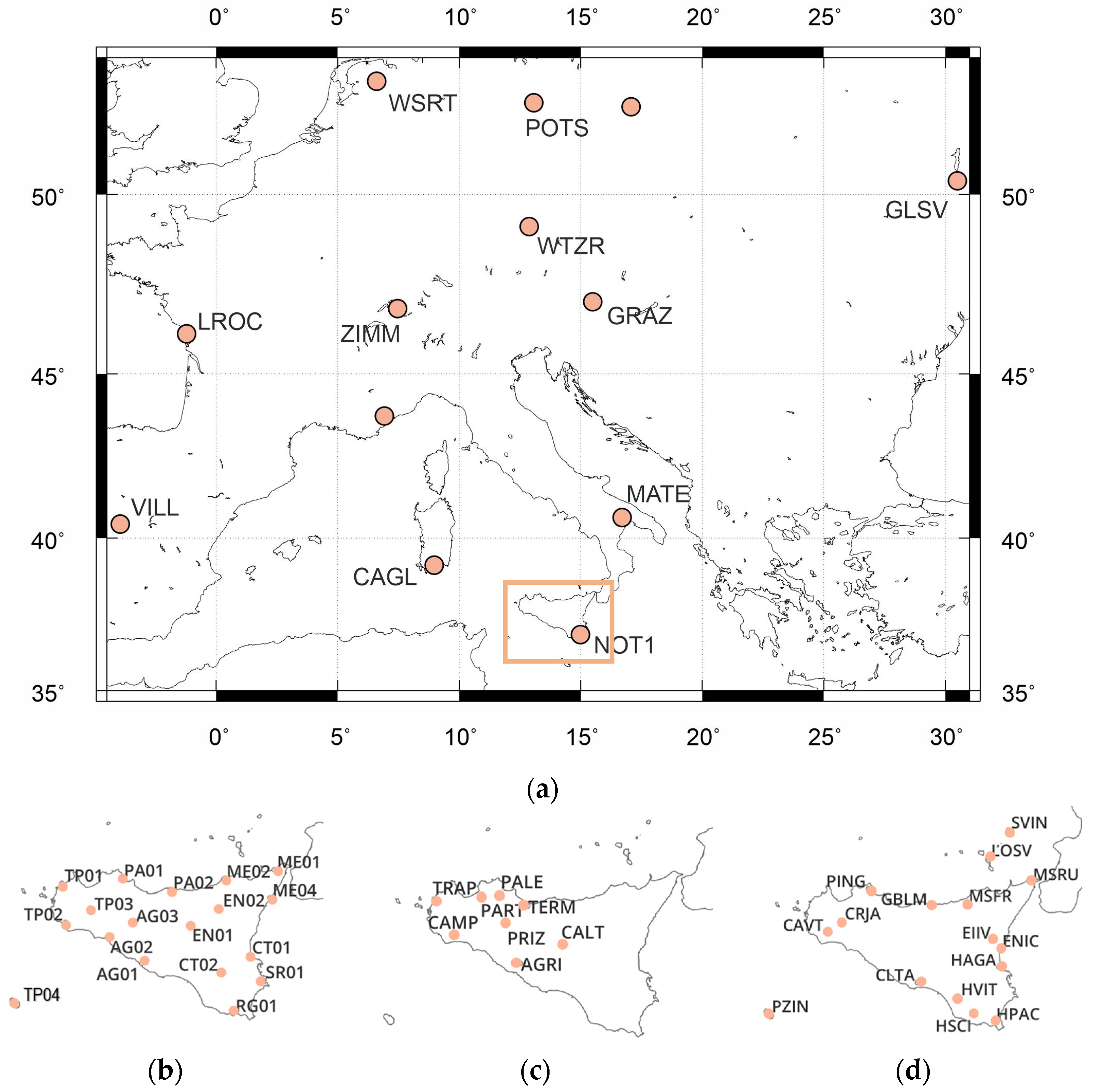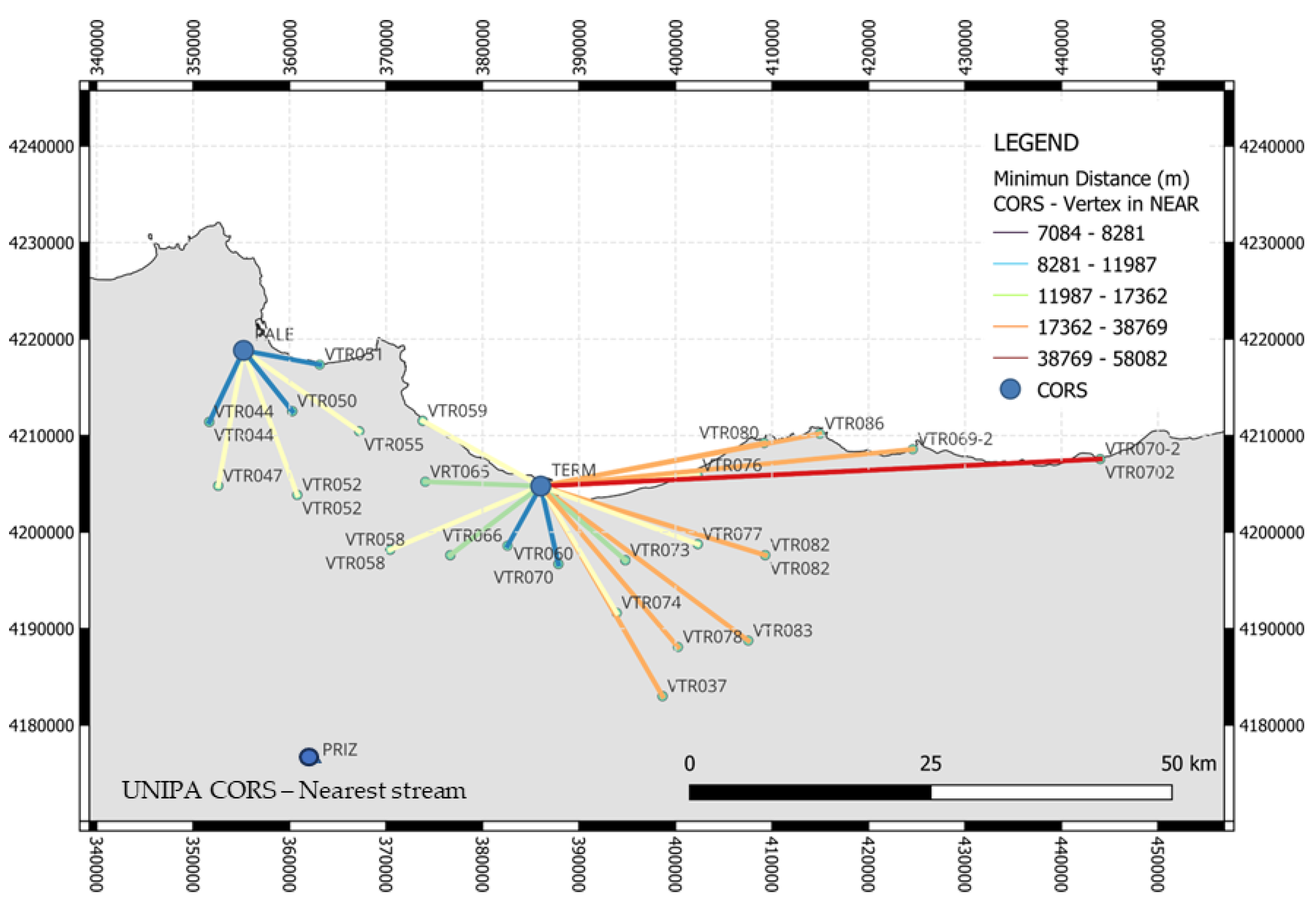Three GNSS CORS networks with different locations, management software and geodetic instruments were thus created in Sicily: the first, in 2007 there has been a private network managed by the Computer Graphics Technologies (CGT) of Palermo, called VRS Sicilia, with Trimble instrumentation, consisting of 18 SPs, framed in the ETRF89 datum, managed by GPSNET software version 2.50, which offers VRS and Nearest as available streams; the second in 2008, the GNSS CORS UNIPA public station network designed and realized by researchers of the University of Palermo, with Topcon instrumentation, was developed, in the framework of the national research project PRIN2005 (networks of GPS permanent stations for real-time surveying in control and emergency deployments), consisting of 8 SPs (Figure 1c), framed in the RDN (Rete Dinamica Nazionale, powered by IGM) ETRF2000 datum, managed by Geo++ software version 2005, VRS, FKP, Nearest available streams [33]; Topcon Positioning Italy, following the collaboration with the University and as part of its commercial activity, has expanded the network by installing other stations in Eastern Sicily; to date, the network has 17 SPs, framed in the IGS05 datum, managed by Geo++ software, streams available VRS, Nea [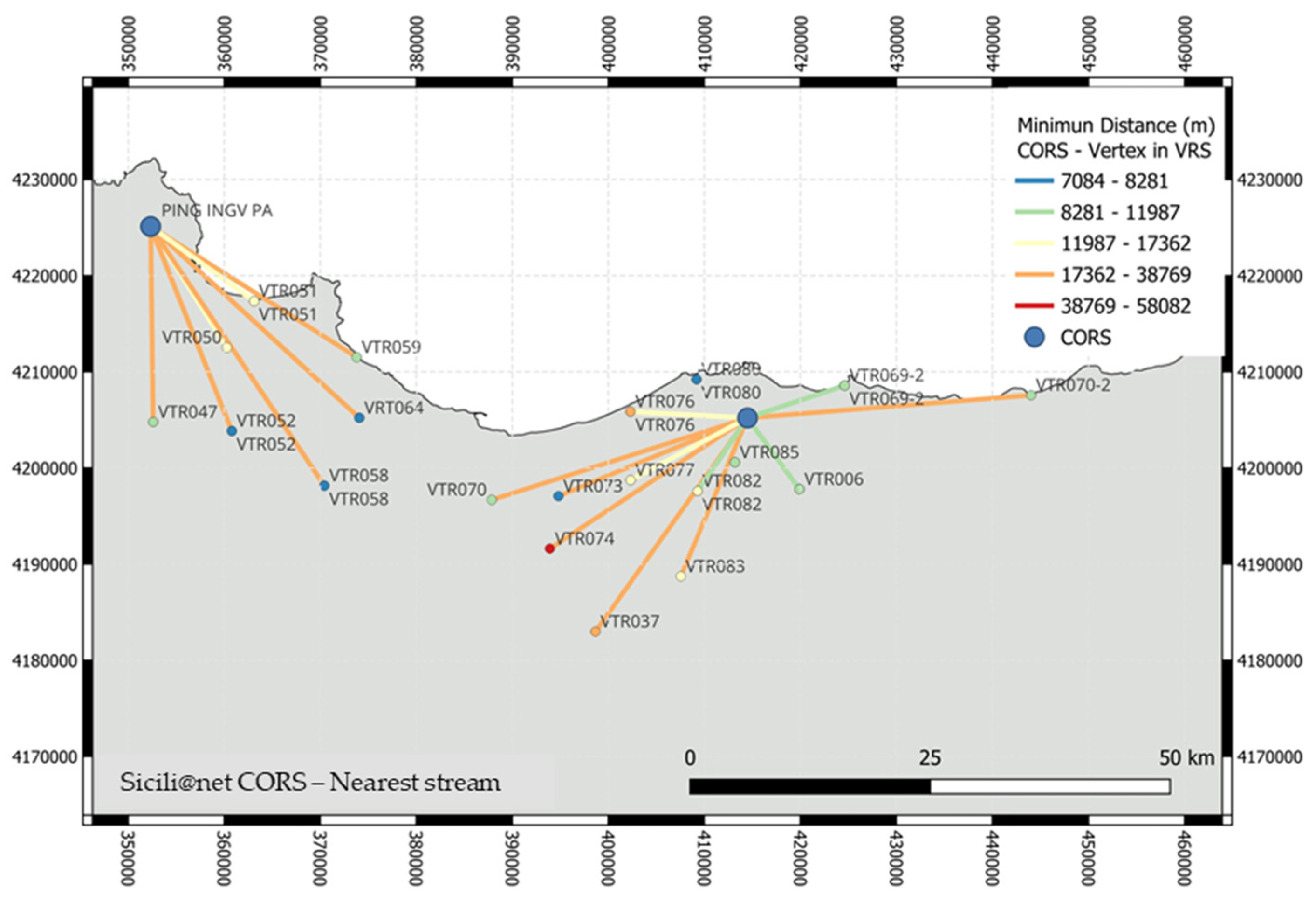34]; the third, since 2009, the INGV has also developed a network of permanent stations for real-time publications called Sicili@net, which relies on some of the 85 CORS managed by the Osservatorio Etneo INGV (INGV OE). This network, consisting of 16 SPs (Figure 1d), with Leica and Trimble instrumentation, is framed in the RDN datum (ETRF2000), managed by the Leica GNSS Spider Net software version 1.0 [30] and offers Max and iMAX, VRS, FKP, and Nearest as available streams. GNSS data are processed by fixing an elevation satellite mask of 10°. Precise IGS (International GNSS Service) Ultra Rapid Orbit is used in the real-time processing that is automatically downloaded; if no precise ephemerides are available, broadcast ephemerides are used. The ionosphere model is fixed to ‘Automatic’, in which GNSS Spider automatically chooses a proper ionospheric model based on the available data. The highest status is given to a model based on the predicted IONEX data, which is downloaded from the IGS. This model is predicted from observations on a global set of GNSS reference stations. It provides the most accurate a priori estimate of the ionosphere’s condition. If this data is not available, the Klobuchar model is used [35]. The Klobuchar model corrects global ionospheric disturbances. In general, it models about 50% of the ionosphere. The parameters needed in the Klobuchar model are provided in the navigation message that is sent from each satellite. The Klobuchar model is applied to the raw observations before the ambiguities are estimated. Furthermore, a standard tropospheric model is applied in data processing. In addition, any tropospheric errors that are not accounted for by the standard troposphere model are estimated by the network processing. This allows network processing to account for unexpected deviations in the tropospheric delay.

Fourth, last but not least, in the Sicilian region, there was also SmartNet ItalPoS managed directly by Leica Geosystem, consisting of 14 SPs, some of which belong to the same INGV network [36].

In Dardanelli et al. [33], all the details concerning the design, data availability, preliminary studies, and analysis involving the GNSS CORS UNIPA network, geodetic framework used, time series of coordinates and displacements retrieved in time, and statistical analysis with the cumulative distribution function (CDF) are shown.

Instead, see the work of Castagnetti et al. [37] for other details of the SmartNet ItalPoS. It is therefore worth pointing out that the GNSS CORS UNIPA and SmartNet ItalPoS networks are now fully operational and form part of the Topcon GNSS [34] and Exagon HxGN SmartNet [36] networks, respectively.

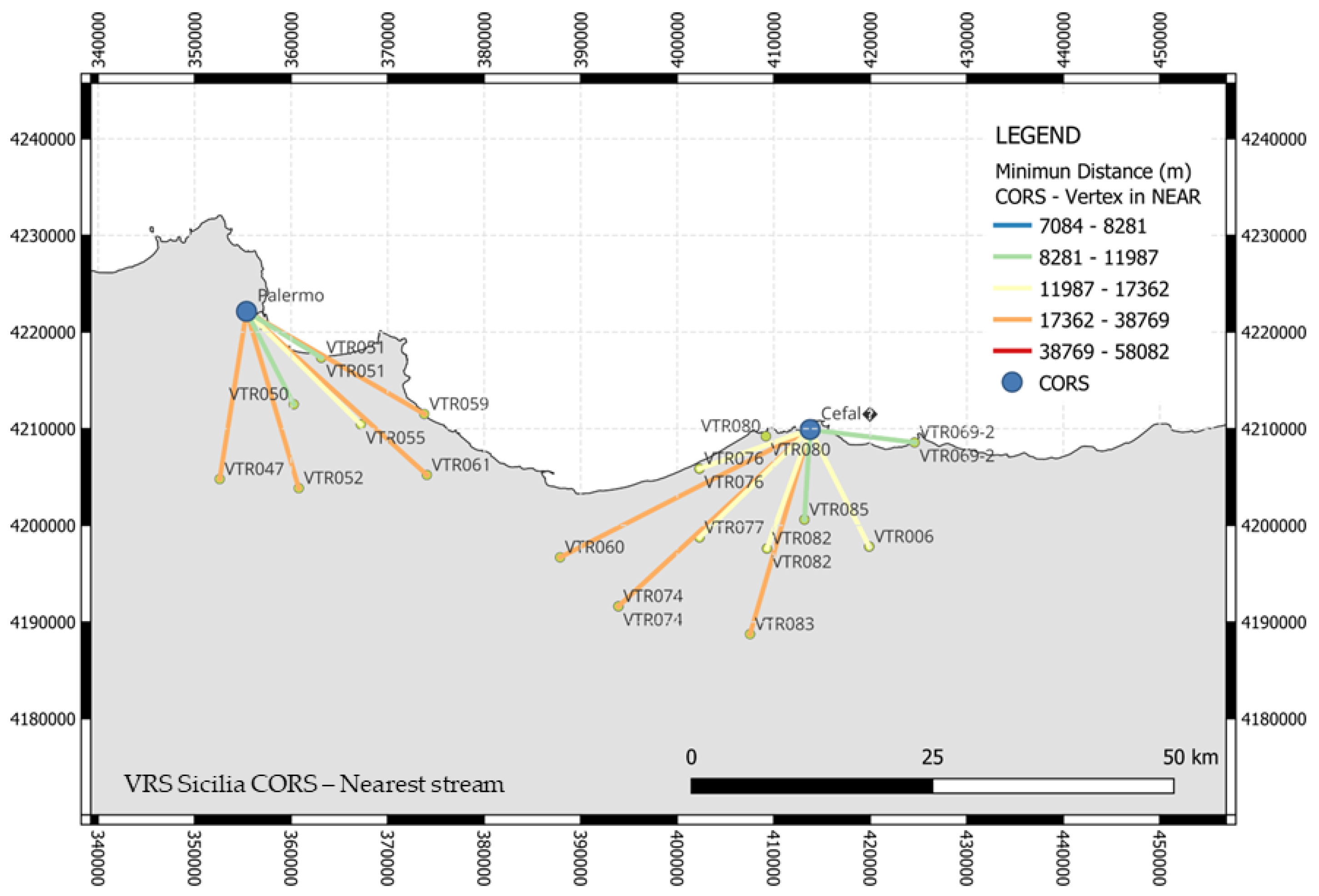
Unlike the networks operated with Topcon and Leica instruments, from 2007 to 2020 the VRS Sicilia network was active on the island (Figure 1b): it consisted of 18 CORS, with Zephir Geodetic II GPS antennas and Trimble^® NetR5 receivers capable of tracking L_1, L_2, L_2 C and L_5 GPS signals, as well as L_1 and L_2 GLONASS. NET TRIMBLE GPS CORS management software. Network service provided corrections: VRS and Nearest.

To determine the geodetic framework of VRS Sicilia, the NDA Professional software (NDA version 2012) has been used. This software has already been used both for the geodetic framework in the GNSS CORS UNIPA network [33] and for other scientific applications. To validate the results of NDA, several adjustments have been carried out over the past years: e.g., Panza et al. compared the results obtained by NDA with those of GAMIT/GLOBK to obtain a combined solution, in the SISMA project (Seismic Information System for Monitoring and Alert), while Dardanelli et al. achieved from NDA performance outcomes that were comparable with Bernese 5.0 [38,39]. Lastly, Maltese et al. 2021 were able to obtain significant results from this software for verification with optical-based classification, thermal diachronic analysis, and a quasi-PS (Persistent Scatter) Interferometric SAR technique in an earthen dam [40]. Therefore, in keeping with what has already been established in the published paper, the following models were used for the processing of the VRS Sicilia network: Saastamoinen tropospheric correction [41,42], the Klobuchar ionospheric correction [35], and the Schwiderski ocean loading correction [43].

In detail, a single baseline was used for the connection between the VRS Sicilia and nearest International GNSS Service (IGS) CORS, CAGL (Cagliari), MATE (Matera) and NOT1 (Noto), represented in Figure 1a in addition to the other IGS stations already used for the geodetic framework of Sicili@net network. For baseline processing, the zenith troposphere estimation (affecting the baseline coordinates estimation) was enabled on both stations (recommended for baselines over 15 km). According to the multi-frequency strategy, double-differenced observation data coming from L5 (wide-lane) and L3 (ionospheric-free) frequency combinations were used. This option is recommended within the software for baseline lengths higher than 10 km. The Least-Squares Ambiguity Decorrelation Adjustment (LAMBDA) method was used to fix the phase ambiguity, as is well known in the work of Teunissen [44]. To estimate the final solution, the wide-lane observation, estimating the wide-lane ambiguity, and then the ionospheric-free observations, estimating the remaining narrow-lane ambiguity, were also used. Finally, the time range and the cut-off angle were set to 30 s and 10 degrees, respectively.

Once the coordinates were calculated in the ITRF2005 system, they were transformed into the ETRF2000 system, using parameters taken from official EUREF documentation (Boucher–Altamimi transformation equations, use of the public website [45]).

Similar to previous studies evaluating permanently materialized CORS, easily accessible and detectable markers were utilized without requiring special arrangements [25]. These GNSS points were selected within the national and local static GNSS networks in Sicily. Specifically, some of the selected points belong to the national network developed during the IGM 95 project, the others to the local GNSS network developed by the Sicilian region. The points from the IGM95 network, developed by the Italian Military Geographical Institute (IGM) in 1990, were calculated in the European datum ETRS89, and they have an interdistance of approximately 20 km and a Root Mean Square Error (RMSE) of ±0.05 m. The points belonging to the regional static local network were mainly developed for technical applications with a spacing of 7–9 km, and an RMSE of ±0.075 m.

When the surveys were carried out, different network SWs were available for postprocessing analyses (Geo++, GNSMART, GPSNEt, Spidernet). Each software has implemented different algorithms for three different network products for real-time survey: data from a virtual station close to the user’s receiver (the so-called VRS approach, in the paper of Vollath et al. [46]), data from an SP and area parameters for spatially correlated disturbances (the so-called FKP approach, in the work of Wübbena et al. [47,48]), corrections for all SPs in the cell surrounding the user (the so-called MAC or MAX, Chen et al. [49].

2.2. Characteristics of the Differential Correction Streams

The acronyms VRS, FKP, and MAX stand for different ways of processing and transmitting network information. Originally, these modes were proposed by individual companies, but later they became standard procedures, partly accepted in the RTCM definitions. As is known, the virtual reference station (VRS) mode requires two-way communication between the user’s receiver and the network center, because the latter has to make specific position corrections for the user’s receiver. The process of combining the data from different stations is performed in the network control center to produce the virtual station data to be sent to the user’s receiver.

The drawbacks of this technique are related to the following aspects: the two-way communication required, a high computational effort of the control center to perform specific calculations for each user, and the requirement of position optimization of the virtual reference station. The latter is necessary to prevent some rovers from using only L1 data, as they received information from a very nearby base station. Of course, this would be appropriate with a real close base station, but not with a virtual one.

The Flachen–Korrectur Parameter (FKP) mode is based on the use of parametric models. The computation is performed by the control center (parameters’ estimation) and the user receiver (position calculation). Indeed, preliminary data from different stations are used to estimate parameters transmitted to the user receiver from the control center. Then, the user receiver performs the optimized position. Compared to the previous method, the FKP mode avoids performing calculations in the control center specific to the user’s receiver; in addition, the transmission could be unidirectional.

The data format of FKP is a proprietary format that exploits the RTCM-2 record 59 left free. In the FPK method, the dispersive effect, i.e., the ionospheric delay, and the frequency-independent effects, where tropospheric delay and orbit errors prevail, are considered separately.

The MAX method was proposed by Leica and Geo++ [48], and the iMAX variant (Individualized MAX) was developed concurrently to accommodate older receivers that were incapable of processing MAX corrections. Nowadays, its format has become part of the RTCM-3 standards. The format is based on data transmission from different reference stations to the user’s receiver without performing any spatial modeling, and the data combination is entrusted to a calculation model that is not strictly defined. The acronym used, ‘Master-Auxiliary’, provides information on network processing based on the differences between the data of a master station (Master) and the remaining stations (Auxiliary). Network processing is easy and does not require a particular model. Also, the MAX system requires the RTCM-3 protocol, and this prevents the use of obsolete receivers.

The iMAX variant provides the information in a format similar to that of the VRS and still uses the RTCM-2 format. Unlike the MAX method, the iMAX mode requires two-way communication. Generally, methods that do not require bi-directional transmission would allow very cost-effective dissemination of information with broadcast-type transmissions based on digital radio technology or similar. Such systems, however, are only experimental. Nowadays, most of the systems are based on a connection between the user’s receiver and the network (direct or via the Internet). Under these conditions, the advantage of a one-to-one system no longer exists [50].

In addition to the differential correction streams mentioned, the Nearest correction has also been involved in the analysis. In this case, the solution is used when the distance between the measured points (VTRs) and the nearest reference station is shorter than approximately 20 km.

2.3. Data Analysis

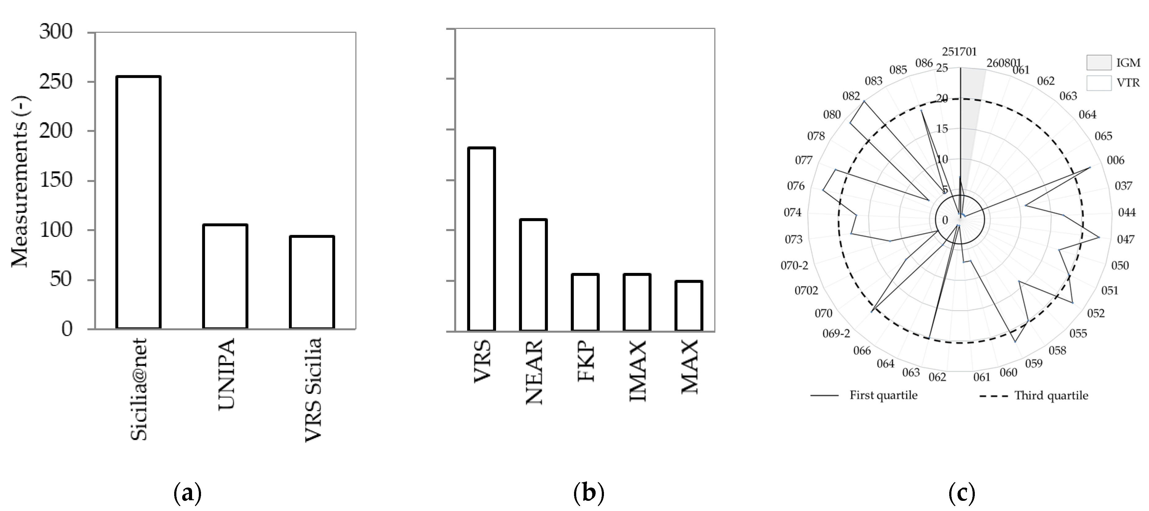
In this work, 455 measurements involving 37 reference points (VTRs) were carried out, employing different CORS networks and streams using NRTK survey. The data consistency of the measurements obtained by using specific guidelines [50] is shown separately in Figure 2, according to the CORS network employed (a), the differential correction streams (b), and then, regardless of the network and the streams involved (c). Considering the consistency of the different CORS networks (panel a), 250 points were measured involving the Sicili@net network, while measurements decreased to ~100 and 90 using the UNIPA CORS network and VRS Sicilia, respectively. Referring to the differential streams, the computation of the solutions with all streams was not possible for all measured points. We reached the most consistent number of measurements with punctual corrections (panel b): ≈180 measurements using the VRS stream, followed by those with Nearest one (≈110 measurements). The measurements obtained involving the areal streams corrections were ≈50 for MAX, IMAX, and FKP. Finally, panel c presents the number of measurements recorded for each VRS point, reported in the vertical axis, obtained using all available CORS networks and data streams. The first quartile, represented in Figure 2c with a black bold circle, corresponds to four measurements, while the third quartile, represented by the dashed circle, corresponds to twenty measurements retrieved from the VTRs and the IGM point. The name of the two IGM points is visualized in the gray sector; the other numbers represent the ID of the VTR points.

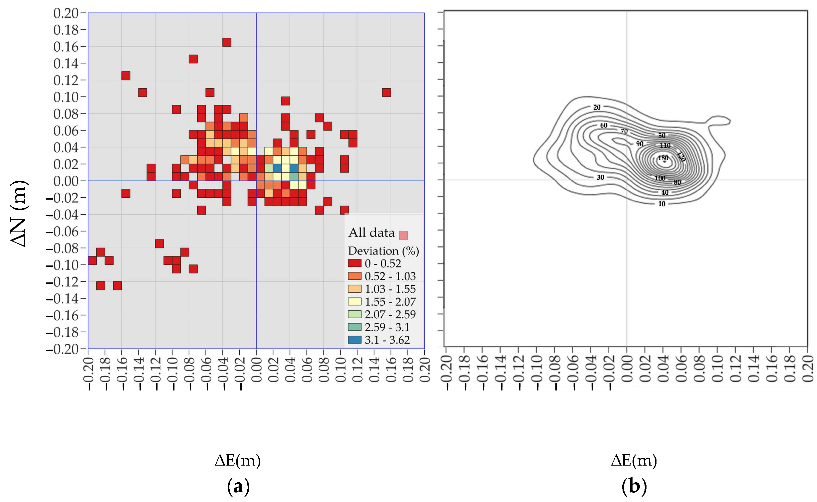
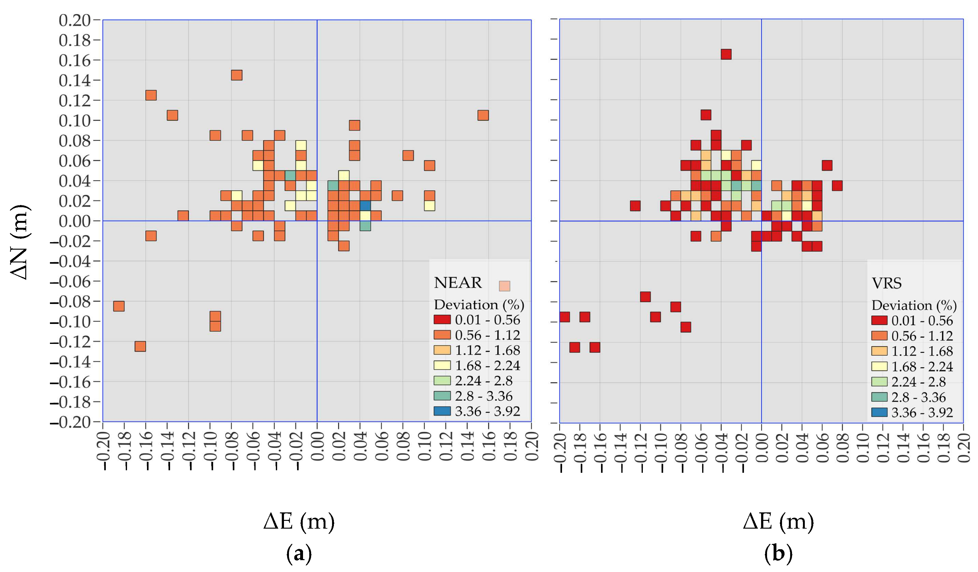
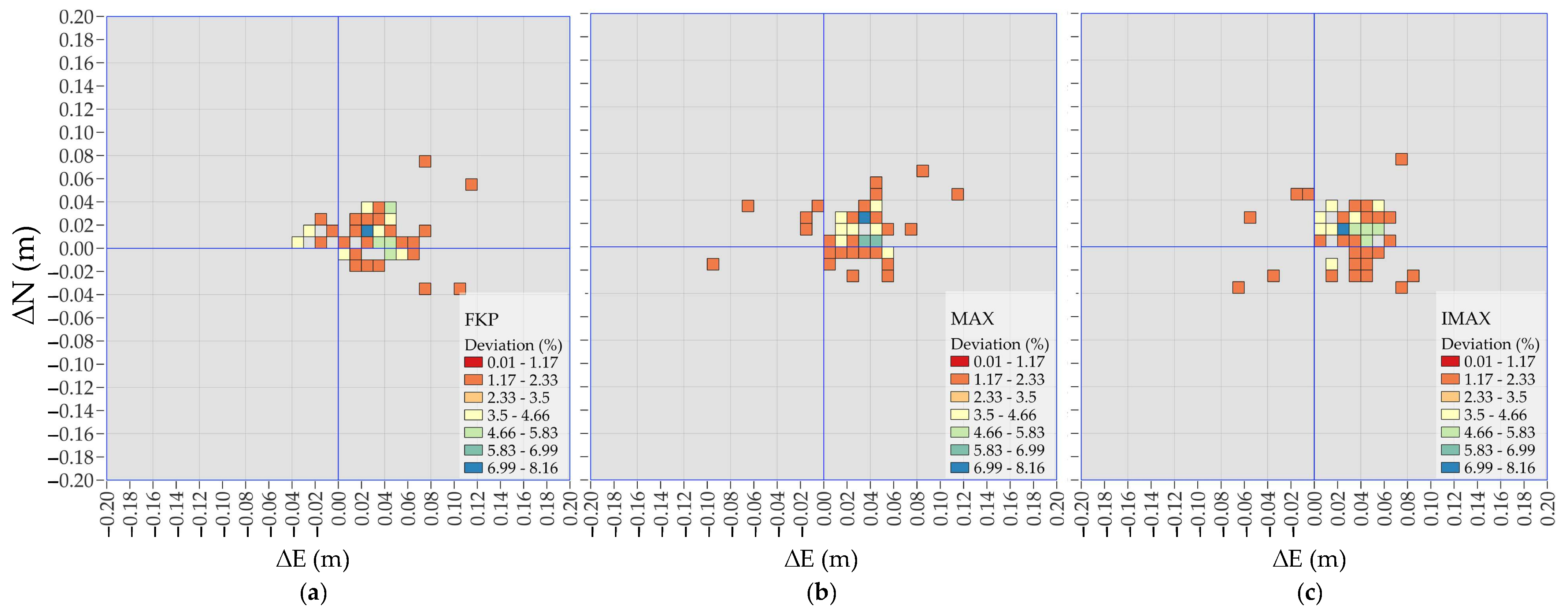
This work evaluates the deviations of the measured points. Preliminary, in a GIS environment, a grid was selected to represent the deviations, analyzing the number of data points falling within each interval; then, the results were separated according to the pattern, as punctual streams solutions (Nearest and VRS) and areal solutions (FKP, MAX, and iMAX).

As is known, the VRS should be considered an areal correction technique. Indeed, it requires multiple reference stations connected to the control center to provide the positioning correction [46]. Since these corrections generate a virtual reference station near the receiver, and the rover processes this data as if it originated from a single reference station, we consider the VRS in this study as comparable to a punctual correction, according to [49]. This provides a basis for comparing it with the Nearest stream, which delivers corrections from the reference station closest to the receiver.

To analyze the empirical distribution of GNSS errors, several statistical tests, among the most representative, have been selected, considering the results for all components in the three directions (∆E, ∆N, ∆Q) separately, and then the planimetric and plano-altimetric components (∆EN, ∆ENQ): Shapiro–Wilk, Cramer–von Mises, Lilliefors (Kolmogorov–Smirnov), Shapiro–Francia, and Anderson–Darling [51].

Razali and Wah conducted a comparative evaluation of the power of various normality tests by analyzing their test statistics relative to critical values. Their findings indicate that the statistical power of these tests is significantly influenced by factors such as the significance level, sample size, and the nature of the alternative distributions. Notably, they observed a non-continuous variation in power, with a critical sample size threshold beyond which test performance changes markedly. Normality tests tend to exhibit reduced power with small sample sizes—typically those of 30 observations or fewer—raising concerns about their reliability in such contexts [52].

Similarly, Mendes and Pala reported that for small sample sizes, the most powerful test may vary depending on the specific sample size, further complicating the selection of an optimal test [53]. In light of these considerations, this study employs a suite of five normality tests to mitigate the limitations of any single method. While individual tests may yield false positives or fail to detect deviations from normality, the combined application of multiple tests is expected to provide a more accurate and comprehensive evaluation of the distributional properties of the GNSS error datasets. Based on the preliminary results, other statistical tests have been performed. Indeed, excluding the normal distribution for some streams, specifically those punctual, the fitting tests involved were some unimodal distributions as Lognormal [54], Weibull [55], and Logistic [56]. The aim was to find whether a unimodal distribution would still fit the patterns obtained. The goodness of the univariate tests was assessed by using the Anderson–Darling (AD) coefficient [57] for the two planimetric and plano-altimetric components ∆EN and ∆ENQ, obtained as a composition of the planimetric and plano-altimetric components, respectively. The lower the AD value obtained, the closer we get to a unimodal distribution.

In the literature, no similar results showing multimodality of GPS processes were found. Some references to multimodality behavior have been retrieved for day–night radiosonde measurement bias data by comparing with zenith tropospheric delay (ZTD) data, as in the papers of Haase et al. [58] and Guerova et al. [59]. Recently, Raghuvanshi and Bisnath verified instances of bimodality for smartphone data, including from Geo++ applications [60], while Xue et al. 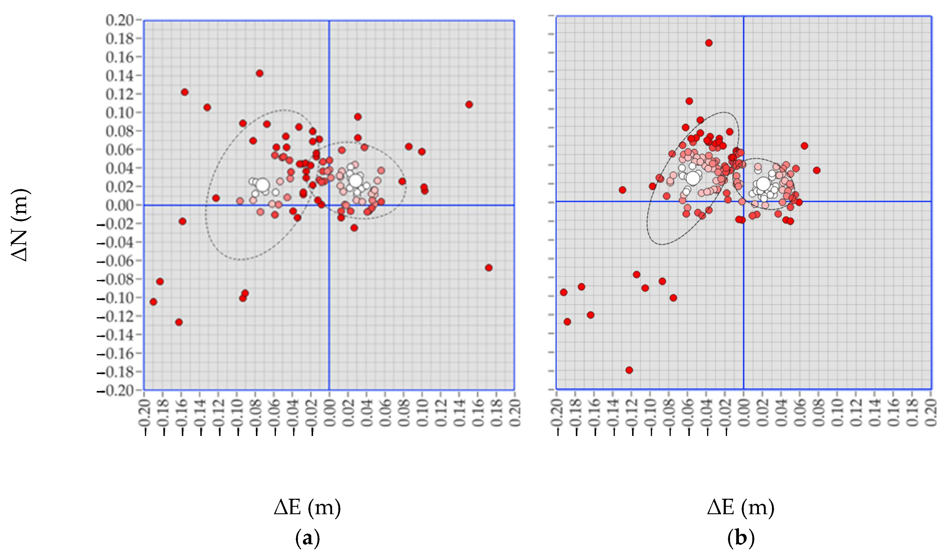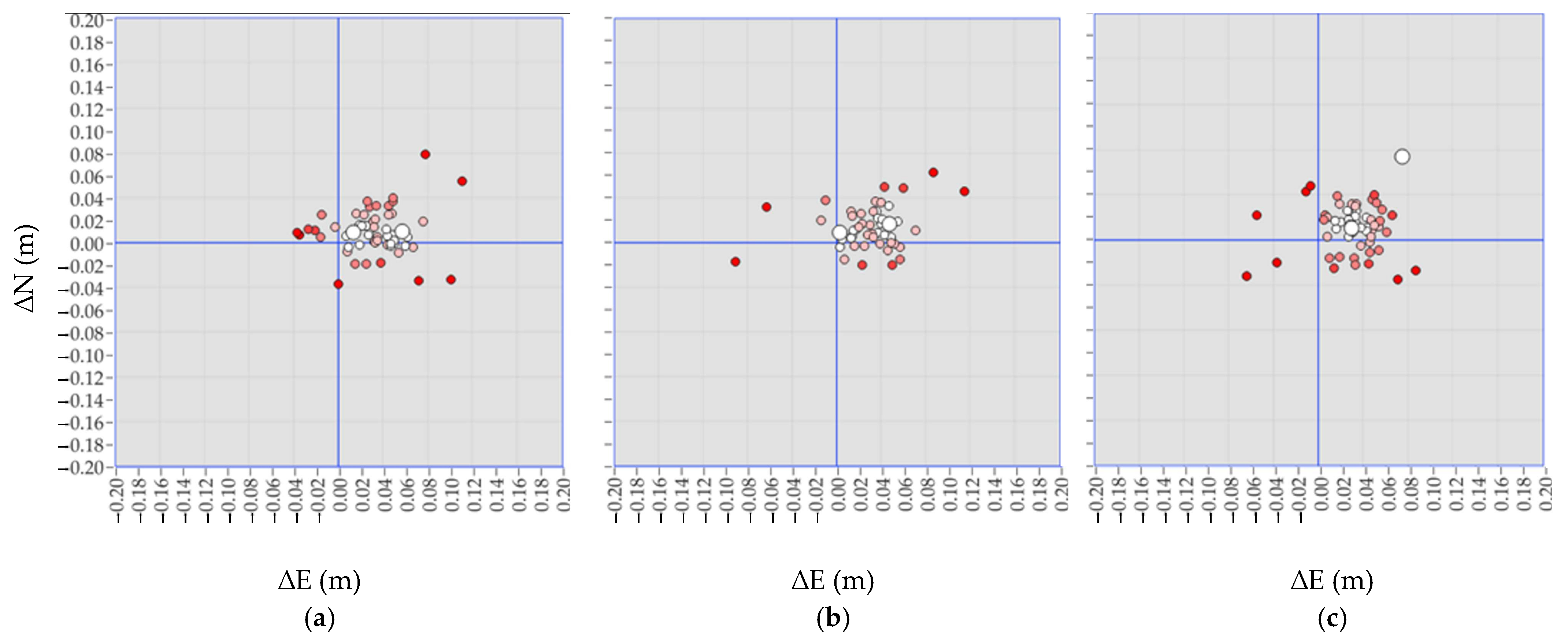found bimodal times for spatial signal ranging errors applied to the GNSS Beidou constellation [61]. To confirm the unusual pattern of the deviations, a Density-Based Spatial Clustering of Applications with Noise (DBSCAN) classification was performed on the geometric position in the domain ∆E − ∆N, for all separated streams [62]. DBSCAN is a non-parametric, density-based clustering method that identifies clusters as contiguous regions of high point density.

Comprehensive descriptions of the algorithm’s theoretical foundations, strengths, limitations, and notable variants are available in the literature [63,64,65]. We selected DBSCAN for this analysis due to its key advantage: it does not require prior specification of the number of clusters. This feature makes it particularly suitable for exploratory spatial data analysis, especially when the underlying distribution is unknown.

In our case study, DBSCAN—executed using the default parameters available in QGIS—identified two clusters in the Nearest, VRS, FKP, and MAX data streams, thereby supporting the hypothesis of bimodality. In contrast, the iMAX stream was predominantly assigned to a single cluster, except for a second cluster consisting of a single outlier point. Additionally, various statistical indicators were extracted and analyzed to quantify the reliability of the results.

The indices involved were the within-cluster deviations (SSW), the between-cluster deviations (SSB), and the total deviations (SST). To account for the heterogeneous sample sizes across streams—reflected in the degrees of freedom within groups (dfw), which were 181, 110, 49, 55, and 55 for the VRS, Nearest, MAX, iMAX, and FKP configurations, respectively—and the number of classes (two per stream, yielding a between-groups degree of freedom, dfb, equal to 1), additional statistical indices were computed. These include the Mean Square Within (MSW) and Mean Square Between (MSB), which were derived accordingly (

Table 1. Univariate normality tests using the Nearest and VRS stream codes for ΔN, ΔE, and ΔQ and the planimetric ΔNE and plano-altimetric ΔNEQ components.

Normality Test	NEAREST					VRS
	ΔN	ΔE	ΔQ	ΔNE	ΔNEQ	ΔN	ΔE	ΔQ	ΔNE	ΔNEQ
Shapiro–Wilk		YES						YES
Cramer–von Mises		YES						YES
Lilliefors		YES						YES
Shapiro–Francia								YES
Anderson–Darling								YES

) and subsequently employed in the calculation of Fisher’s F-statistic.

Two additional statistical tests have been performed to finalize the analysis: the ANOVA and Ashman’s D coefficient analysis. The ANOVA statistical test has been evaluated to determine the probability that the calculated F-value and the critical F-value match. The latter depends on the classes and the sample size used. Since the analyses involve different sample sizes for each stream, an unbalanced F-value was also considered, as required in these cases. The probabilities obtained for each stream were compared with the minimum likelihood obtained from the stream’s solutions. The Ashman’s D coefficient (Equation (1)) was calculated separately for the variables ∆E and ∆N using the following equation:

$$D={\displaystyle \frac{\mid \mu 1-\mu 2\mid }{\sqrt{\left(2\right({\sigma }_1^2+{\sigma }_2^2)}}}$$

(1)

The test based on Ashman’s D coefficient aims to check whether the distribution is bimodal and whether the two peaks are distinct from each other. To this aim, the coefficient D must be >2.

As a final investigation, a linear multiple regression analysis was performed to quantify the influence of several parameters on the distribution response.

The parameters included in the correlation analysis were the distance between the VTRs and the nearest CORS reference stations (d), the distance between the VTRs and the coastline and the altimetry of the measured VTRs (d_s, h) to consider a residual tropospheric effect, and finally the horizontal and vertical root mean squares (σ_h and σ_v, respectively) to consider the satellite geometric configuration at the time of measurement acquisition. The contribution related to the distance between the VTRs and the nearest CORS reference stations providing the correction was made only for the Nearest stream. The same approach was not carried out for the VRS stream, as we do not know the location of the virtual station, still materialized virtually within a few km from the measured VTRs, according to [46]. The value of the Pearson coefficient r [66] indicates the strength of a linear relationship between the empirical and the corresponding values. According to the r values, the correlation varies from very weak (r < 0.2) to very strong (r > 0.8). While equal sample sizes are ideal for maximizing statistical power and robustness, they are not a strict requirement for the statistical tests employed in this study.

Specifically, ANOVA can accommodate unequal sample sizes, although this may affect the test’s sensitivity to violations of homogeneity of variances. In our analysis, assumptions were verified [67]. Provided that, balanced ANOVA assumes equal sample sizes across groups and provides a straightforward interpretation of main effects and interactions; however, when sample sizes differ—as in our case, where the number of observations ranged from approximately 50 to 180 per stream—unbalanced ANOVA could help strengthen the results by adjusting for unequal group sizes [68,69].

Ashman’s D coefficient, used to assess bimodality, is based on the separation between two distributions and remains valid as long as group statistics (means and standard deviations) are reliably estimated [70].

The normality tests applied—Shapiro–Wilk, Cramér–von Mises, Lilliefors (Kolmogorov–Smirnov), Shapiro–Francia, and Anderson–Darling—are all applicable to samples of varying sizes. While their power may vary with sample size, they remain statistically valid across the range used in this study [51,52].

Similarly, goodness-of-fit tests for unimodal distributions (Lognormal, Weibull, Logistic) are robust to unequal sample sizes, provided that expected frequencies are adequate [71].

In our dataset, the number of measurements per stream ranged from approximately 50 to 180. These sample sizes reflect the realistic operational conditions; therefore, we retained the natural sample distribution to preserve the integrity of the observational data and limit artificial balancing that could introduce bias.

3. Results

3.1. Deviations’ Cluster Analysis

As a first step, we examined the planimetric deviations (∆N and ∆E) from the measurements gathered during the NRTK survey.

These were grouped regardless of the CORS network from which the corrections were applied (UNIPA, Sicili@net, VRS Sicilia) and regardless of the stream implemented (Nearest, VRS, FKP, MAX, and iMAX).

We divided the deviation range into 0.01 m bins and tallied the number of points in each interval, thereby quantifying the deviation density and identifying the bins with the highest observations.

A pseudo-color representation of the data clustered into seven classes was selected, characterized by ‘natural breaks’ (Figure 3a). The representation in the left panel seems to highlight two main clusters and shows a non-typical Gaussian distribution of errors.

To further highlight these findings, Figure 3b presents an additional image using the same axes and scale. In this figure, the contour lines, obtained by interpolating the deviation density, confirm the possibility of a multimodal pattern of the planimetric errors. Thus, for the following analyses, we will only refer to the binning.

According to these preliminary results, we first focused on the planimetric errors regardless of the CORS networks involved. Then we separated the punctual and GNSS data streams code (Nearest and VRS) from the areal ones (FKP, MAX, and iMAX). In the following panels, different scales have been used to represent the results for punctual and areal streams, to describe the intra-group variability, and to make the comparison between the various streams.

From this discrimination, the multimodal distribution of the errors already obtained for the whole dataset is now mainly retrieved only for the Nearest and VRS streams codes (Figure 4a,b, respectively). In both panels, two clusters are clearly separated, according to the results shown in Figure 2a, while the pattern changes for the areal streams (Figure 5a–c).

3.2. Statistical Analyses of Deviations’ Distribution

Given the frequent use of the Gaussian distribution in GNSS analyses [25], the normality of all data was tested, considering the various streams involved. The univariate tests on the different components involved (∆N, ∆E, ∆Q, ∆NE, and ∆NEQ) were chosen among the most representative: Shapiro–Wilk, Cramer–von Mises, Lilliefors (Kolmogorov–Smirnov), Shapiro–Francia, and Anderson–Darling. The results would validate that for the punctual techniques, the distribution is not normal, except for the ∆Q component of the VRS stream (Table 1). On the other hand, the normal distribution fits approximately well for some of the areal techniques and not for all components: ∆N, ∆E, ∆Q, and ∆NEQ for FKP, ∆NE, and ∆NEQ for iMAX (

Table 2. Univariate normality tests using the FKP, MAX, and IMAX stream codes for ΔN, ΔE, and ΔQ and the planimetric ΔNE and plano-altimetric ΔNEQ components.

Normality Test	FKP					MAX					iMAX
	ΔN	ΔE	ΔQ	ΔNE	ΔNEQ	ΔN	ΔE	ΔQ	ΔNE	ΔNEQ	ΔN	ΔE	ΔQ	ΔNE	ΔNEQ
Shapiro–Wilk	YES	YES	YES		YES	YES					YES				YES
Cramer–von Mises	YES	YES	YES		YES				YES					YES	YES
Lilliefors	YES	YES	YES		YES			YES	YES					YES	YES
Shapiro–Francia		YES	YES		YES	YES									YES
Anderson–Darling	YES	YES	YES		YES									YES	YES

).

Since the normal distribution was excluded for certain streams, particularly punctual ones, we conducted alternative fitting tests using unimodal distributions such as Lognormal, Weibull, and Logistic. The objective was to determine whether a unimodal distribution could still fit the observed patterns. The goodness of the bivariate tests was evaluated using the Anderson–Darling (AD) coefficient for the two variables, ΔEN and ΔENQ, derived from the composition of planimetric and plano-altimetric variables. The lower the AD value obtained, the closer we get to a normal-type distribution. As expected, the AD coefficient provided higher values for the punctual corrections (

Table 3. Goodness-of-fit test for unimodal distributions for the planimetric component ΔNE, analyzing all correction streams and the Nearest and VRS correction streams separately.

Distribution	ALL		NEAREST		VRS
	AD	P	AD	P	AD	P
Lognormal	2.466	<0.005	0.342	0.488	1.485	<0.005
Weibull	9.373	<0.010	2.064	<0.010	3.952	<0.010
Logistic	8.701	<0.005	3.344	<0.005	2.843	<0.005

and

Table 4. Goodness-of-fit test for unimodal distributions for the plano-altimetric component ΔNEQ, analyzing all correction streams and the Nearest and VRS correction streams separately.

Distribution	ALL		NEAREST		VRS
	AD	P	AD	P	AD	P
Lognormal	1.058	0.009	0.508	0.196	0.504	0.201
Weibull	2.622	<0.010	0.867	0.024	0.826	0.033
Logistic	5.184	<0.005	1.699	<0.005	2.054	<0.005

) than for the areal ones (

Table 5. Goodness-of-fit test for unimodal distributions for the planimetric component ΔNE, analyzing the areal correction streams.

Distribution	FKP		MAX		iMAX
	AD	P	AD	P	AD	P
Lognormal	0.671	0.075	1058	0.008	0.678	0.073
Weibull	0.992	0.012	0.482	0.23	0.52	0.195
Logistic	0.743	0.03	0.372	>0.250	0.264	>0.250

and

Table 6. Goodness-of-fit test for unimodal distributions for the plano-altimetric component ΔNEQ, analyzing the areal correction streams.

Distribution	FKP		MAX		iMAX
	AD	P	AD	P	AD	P
Lognormal	0.349	0.464	0.932	0.017	0.491	0.211
Weibull	0.347	>0.250	0.719	0.057	0.429	>0.250
Logistic	0.525	0.139	0.98	0.006	0.312	>0.250

), for all unimodal distributions analyzed except for the Lognormal distribution.

This result confirms that the distribution along both the planimetric component ∆EN and the plano-altimetric component ∆ENQ of the punctual streams is not strictly unimodal (Table 3 and Table 4, respectively). In the same tables, the highest values in bold for both ∆EN and ∆ENQ components were obtained considering all streams.

To verify these results, other statistical tests, focusing specifically on the bimodal distribution, were conducted as two distinct clusters were identified in prior analyses. Our study aims to highlight this atypical behavior within the dataset, suggesting potential scenarios that could explain its occurrence.

3.3. Classification of the Deviations’ Clusters

A DBSCAN classification was performed on the geometric position in the domain ∆E − ∆N, for all streams considered separately, establishing a priori the separation into two different classes. The validation of the test was carried out by analyzing some statistical indicators and through the visual interpretation of the clusters obtained by the classification. Referring to the latter, in Figure 6 and Figure 7, we represented the different classes, obtained by the classification, as a function of the distance from the respective centroids. A pseudo-color representation was performed in a GIS environment. Specifically, the largest white point represents the mean value, defined as the cluster centroid; the other points represent the distance from the centroid. Also, in Figure 6a,b, two confidence ellipses (±3σ away from the centroid) have been overimposed on the clusters to help highlight the separation between the two different groups obtained once again for the punctual streams. Indeed, the visual interpretation seems to confirm that the two clusters are almost separated from each other, and the distribution is therefore not unimodal.

On the contrary, analyzing the clusters obtained for the areal streams (Figure 7), the two classes obtained by the classification are not clearly separated; also, for FKP and MAX streams, the corresponding centroids seem to be closer to each other (Figure 7a,b, respectively). Given the smaller sample size within each cluster classified by streams, we opted not to represent the confidence ellipses.

The iMAX correction technique, represented in Figure 7c, was the only one with a completely different pattern compared to the other streams. Specifically, from the classification results, the two classes were identified by n-1 points and only 1 point, respectively, where n represents the population analyzed for that stream. Thus, the class identified by a single point is represented by a single centroid in a position quite separate from the other points. This result suggests that the distribution for iMAX could be interpreted as unimodal, indicating that two distinct classes cannot be distinguished. Therefore, no further statistical analysis will be carried out on this stream.

The statistical analyses performed on the other streams aimed to quantify the real existence of two distinct clusters. The indices involved from the classification process are the within-cluster deviations (SSW), the between-cluster deviations (SSB), and the total deviations (SST). Additional indices were also calculated to consider the sample sizes, different for each stream and the classes (2 for all streams). These are the Mean Square Within (MSW) and Mean Square Between (MSB), respectively (

Table 7. ANOVA test and Ashman’s D coefficient analysis.

	VRS	NEAR	MAX	FKP
SST	0.696	0.646	0.067	0.072
MSB	0.2573	0.2738	0.0242	0.0263
MSW	0.0024	0.0034	0.0009	0.0008
F	105.6	80.2	27.1	31.3
Funbalanced	107.2	80.5	26.9	33.8
P/Pmin	2.2 × 10−14	2.2 × 10−9	1.0 × 10+00	1.6 × 10−1
Ashman’s D (ΔE)	12.958	12.576	0.9208	11.099
Ashman’s D (ΔN)	0.0798	0.0537	0.2125	0.0195

), used for the Fisher’s coefficient (F) computation.

Once again, Table 7 shows that the Nearest and VRS streams have a different behavior than the areal streams analyzed (MAX and FKP only). The ANOVA analysis was performed to determine the probability that the calculated F-value and the critical F-value match. The latter depends on the classes used and the sample size. Since the analyses involve different sample sizes for each stream, an unbalanced F-value was also considered, as required in these cases. However, as reported in Table 7, the unbalanced coefficient does not differ much from the calculated F-values.

The probabilities obtained for each stream were compared to the minimum likelihood, which, in this case, was determined using the MAX stream.

From the analysis, the probabilities found for Nearest and VRS streams result very low, indicating that the classes produced by the classifier are dissimilar to each other or at least more different than the classes obtained for the areal correction techniques.

We also summarize in the same table the results of an additional univariate statistical test involving Ashman’s D coefficient, which was calculated separately for the variables ΔE and ΔN.

The test aims to check whether two distributions exist and whether they are distinct from each other. To this aim, the coefficient D must be >~2.

As shown in Table 7, this threshold was not reached for either component or any of the analyzed streams. However, we observed a moderate separability between the classes for ΔE, although not clearly defined, as indicated by the higher values in the punctual streams compared to other techniques. Additionally, the values exceeded 1. Conversely, in the analysis of the ΔN component, all values remained lower than those obtained for ΔE and were close to zero.

3.4. Estimation of the Correlation Between the Parameters Involved in the Analysis

Thus, for all streams, we are not able to detect a clear separability between the classes. These results are probably related to the dominant distribution of the measured points along the E-W direction. In fact, along the E-W direction, the maximum distance between the VTRs is approximately 90 km, whereas along the N-S direction, it is 40 km. Considering only the CORS, the maximum distance between the stations involved is 50 km along the E-W direction and about 20 km along the N-S direction. Considering the distances between the VTRs and the CORS involved separately, these ranged from 7 to ~60 km (Figure 8, Figure 9 and Figure 10). A pseudo-color representation of the distances clustered into five classes was chosen, characterized by ‘natural breaks’ (Jenks algorithm).

All the analyses performed seem to confirm that the distribution of the Nearest and VRS streams is not unimodal. Based on the results of Ashman’s D coefficient and the distances between the VTRs and the CORS reference stations, a further investigation was made to test how this latter, and other parameters discussed below, may influence the distribution response according to the CORS used. To quantify this correlation, a linear multiple regression analysis was performed. The variables analyzed refer to the distance between the VTRs and the nearest CORS reference stations (d), the distance between the VTRs and the coastline and the altimetry of the measured VTRs (d_s, h) to consider a residual tropospheric effect, and finally the horizontal and vertical root mean squares (σ_h and σ_v, respectively) to consider the satellite geometric configuration at the time of measurement acquisition.

The contribution related to the distance between the VTRs and the nearest CORS reference stations—those providing the correction—was evaluated only for the Nearest stream. The results were separated according to the CORS involved (

Table 8. Pearson’s coefficient values using the Nearest stream correction, involving different parameters: the distance (d), the distance between the VTRs and the coastline, and the altimetry of the measured VTRs (d_s, h) and the horizontal and vertical root mean squares (σ_h and σ_v, respectively). Weak correlations in gray, strong correlations in black bold; very weak correlations were omitted.

	ΔEN vs.	ΔENQ vs.	ΔEN vs.	ΔENQ vs.	ΔEN vs.	ΔENQ vs.
r (-)	d	d	(ds, h, d)	(ds, h, d)	(σh, σv, ds, h, d)	(σh, σv, ds, h, d)
VRS Sicilia	0.428	0.483	0.465	0.516	0.595	0.709
UNIPA			0.288		0.294
Sicili@net				0.202		0.209

).

A similar approach was not applied to the VRS stream, as the exact location of the virtual station remains unknown. However, according to [44], it is virtually materialized within a few kilometers of the measured VTRs.

Thus, the comparison between the two streams was made by considering only the variables common to both streams (

Table 9. Comparison between Pearson’s coefficient values using the Nearest and the VRS stream corrections, involving different parameters: the distance (d), the distance between the VTRs and the coastline and the altimetry of the measured VTRs (ds, h) and the horizontal and vertical root mean squares (σ_h and σ_v, respectively). Weak correlations in gray, moderate correlations in black; very weak correlations were omitted.

r (-)	ΔEN vs. (ds, h)		ΔENQ vs. (ds, h)		ΔEN vs. (σh, σv)		ΔENQ vs. (σh, σv)		ΔEN vs. (σh, σv, ds, h)		ΔENQ vs. (σh, σv, ds, h)
	NEAR	VRS	NEAR	VRS	NEAR	VRS	NEAR	VRS	NEAR	VRS	NEAR	VRS
VRS Sicilia			0.009		0.192	0.386	0.209	0.293	0.201	0.408	0.356	0.331
UNIPA	0.283	0.042				0.286			0.293	0.286
Sicili@net			0.202	0.276							0.209	0.281

). For both analyses (Table 8 and Table 9), r values below the 0.2 threshold, providing a very weak correlation, were omitted because their contribution is not relevant for the analysis. Specifically, when comparing the two streams in Table 9, the correlation is predominantly weak, except for the VRS Sicilia network, where it becomes moderate for the VRS stream.

Analyzing the contribution of the distance between the VTRs and the nearest CORS reference stations, only for the Nearest stream, in Table 8, the coefficient r results generally moderate, considering only the VRS Sicilia CORS. The correlation becomes strong for the same CORS if all parameters are included in the analysis, for both planimetric and plano-altimetric components (r = 0.6 and r = 0.7, respectively). The r values for the remaining CORS are low, and the corresponding correlation is mainly weak and very weak. Since high correlations were not obtained in any case when analyzing the contribution of individual variables, this suggests that the results may be influenced by residual errors that were likely not resolved during processing. Furthermore, these findings suggest that multiple factors could influence the distribution’s behavior, contributing to its non-uniformity

4. Discussion

The assumption of a normal distribution of the deviations is commonly accepted in the literature for GNSS analyses. In this study, this seems to be confirmed when areal corrections (FKP, MAX, iMAX) are applied to the GNSS NRTK solutions. On the contrary, when punctual correction streams are involved (Nearest and VRS), the pattern seems to perform a multimodal distribution.

These assumptions have been represented in a GIS environment, distinguishing the results obtained from the CORS networks, considering the streams and the CORS all together, and then when punctual and areal corrections streams are applied separately. The results confirmed that the multimodal distribution obtained for the whole dataset considering the whole streams is mainly due to the contribution of the punctual correction techniques, as represented in Figure 4a,b. When the areal corrections are applied, we are not able to distinguish clearly between the two different groups; rather, the distribution of the errors seems to be more homogeneous. The use of different statistical tests involved in this study aims to analyze the results obtained via GIS and determine whether other distributions different from the normal one could be related to the results.

To confirm the non-normality of some distributions, several univariate tests were chosen among the most representative to be applied along the three components and their combination. The results confirmed that when the punctual corrections are applied, the distribution is not normal, except for the ∆Q component of the VRS stream. The normal distribution could be approximately suitable for some areal streams but not for all components: ∆N, ∆E, ∆Q, and ∆NEQ for FKP, ∆NE, and ∆NEQ for iMAX. Assuming the non-normality of some distributions, other tests have been performed as the Lognormal, Weibull, and Logistic unimodal distributions, to fit the GNSS distributions. The goodness of the bivariate tests was assessed through the AD coefficient for both the planimetric and plano-altimetric components. The lower the AD value obtained, the closer we get to a normal-type distribution. As expected, the AD coefficient provided higher values for the punctual corrections than for the areal corrections for all unimodal distributions analyzed, except for the Lognormal distribution.

Applying the DBSCAN algorithm without a priori assumptions regarding the existence of two distinct classes—as previously suggested by preliminary analyses—visual inspection of the clustering results once again reveals a clear separation between two clusters, indicating a non-unimodal distribution. The positioning of the corresponding centroids further highlights this inter-cluster distinction. However, this separation becomes less evident when spatial corrections are introduced, particularly under the application of the iMAX stream, wherein the dataset appears to form a single homogeneous class. Notably, the two clusters identified via DBSCAN have also been examined through alternative statistical methodologies. Specifically, several indices have been involved in the ANOVA analysis and Ashman’s D coefficient computation. The first test aims to determine the correspondence between the calculated Fisher value and the critical value, considering the classes used and the sample size. The probabilities of each stream were compared with the minimum likelihood obtained in our case for the MAX stream.

The results for the Nearest and VRS streams were very low, indicating that the classes identified by the classifier are significantly different from one another. Ashman’s D coefficient was calculated separately for the ΔE and ΔN components to assess whether two distinct distributions exist. For this purpose, the coefficient D should be approximately 2. This threshold was not reached for either component across all analyzed streams.

However, along ∆E, the highest results were obtained for punctual streams reaching values greater than 1. In contrast to this assumption, along ∆N, the values are still lower than those obtained for ∆E and close to zero. So, in this case, the distinction between the two classes is not clearly evident, maybe for the main distribution of the VTRs and CORS along the E-W direction, instead of along the N-S direction.

In order to quantify the real influence of the distance between the VTRs and the CORSs and investigate the alignment along the main directions E-N of the VTRs and CORS distribution, further analyses have been performed, involving a multiple regression analysis. These focus on the correlation between different parameters involved in the solution determination, such as the mentioned station distances, residual tropospheric effects, and the satellite geometric configuration at the time of measurement acquisition. The results showed a predominantly weak and very weak correlation for all CORS, except for one, for which the correlation is moderate.

For the same CORS, the correlation became strong across all parameters, with values of r = 0.6 for the planimetric component and r = 0.7 for the plano-altimetric component.

Since high correlations were not obtained in any case when analyzing the contribution of individual variables, this suggests that the results may be influenced by residual errors that were likely not resolved during processing. Furthermore, these findings suggest that multiple factors could influence the distribution’s behavior, contributing to its non-uniformity. About the accuracy of the measured points considering their position in this study, and specifically the alignment along the E-W direction, and the density close to the CORS stations along the shoreline in the N-S direction, we can relate the retrieved behavior to that mentioned in the study by Dabove et al. [70]. The authors used two different network software solutions, as in this study—GNSMART by GEO++ and Spidernet by Leica Geosystems—and examined the reliability of Virtual RINEX (VR). The latter is a standard product for postprocessing data (GNSS) when the distance between the rover and the master is greater than 30 km (as in our case), generated by the software’s algorithms to calculate and model the bias. Also, similarly to our analysis, the quality and accuracy of positioning were assessed near the boundaries of two different regions in Italy. Two CORS networks were employed, with an interdistance of approximately 40 km between the SP (typical for Italian networks), and measurement points were distributed close to the boundary between the two networks. The results demonstrated the different behaviors of the two software in generating VR, leading to positioning results that can vary by tens of centimeters. An important role could be attributed to the morphological conditions of the networks, as in our case [72]. Analyzing the behavior of networks close to the limits of different regions, Garrido et al. [73] and Giménez et al. [28] found that the influence of neighboring active networks on measured points in that area is a critical issue. The authors presented the results of post-processed and simultaneous NRTK positioning for several test points situated in the border region between Portugal and the Andalusian Community, in the southwestern Iberian Peninsula. The analysis was based on two active GNSS networks present in this border region, a national RTK network and a local one, with similar interdistances and features. By comparing the post-processed positions for each test point across both analyzed active networks, differences of less than 2 cm were observed for the east and north components, while the up component showed deviations of up to 4 cm.

5. Conclusions

This work aims to analyze the distribution of the deviations of the positioning of several reference VTRs, whose coordinates were already known. The comparison of results considered not only the various CORS networks used for the measurements but also analyzed the influence of different correction streams on NRTK surveys.

More generally, results demonstrated a multimodal pattern for both Nearest and VRS streams, comparable with the results of all data considered as a whole. The multimodal distribution is not predominant when areal corrections are applied. Thus, several statistical tests have been performed to assess this pattern. The tests confirmed that the distribution of the errors could be considered normal when areal corrections are applied, while when the Nearest and VRS are involved, the normality of the solution cannot be considered. Among different unimodal distributions, three representative non-normal distributions have been chosen to confirm the non-normality of the GNSS solutions in this study. As expected, the result seems to confirm that when punctual corrections are involved, the distribution along both the planimetric and the plano-altimetric components is not strictly unimodal. The presence of two distinct classes, and a bimodal error distribution—particularly evident when punctual correction streams are applied—is corroborated by the clusters identified via the DBSCAN algorithm in the (ΔE, ΔN) domain. As DBSCAN does not require prior knowledge of the number of clusters, it enables an unbiased classification. The results, further supported by the representation of class-specific centroids, confirm that solutions employing punctual streams exhibit a clear separation into two distinct clusters. In contrast, the clusters associated with FKP and MAX correction streams demonstrate limited separation, with their centroids located in closer proximity. For the iMAX correction stream, a unimodal distribution is observed, indicating that the assumption of two separate classes is not applicable in this case.

In the last analysis, the correlation between the parameters involved in the solution has been investigated. For both planimetric and plano-altimetric components, a very weak and weak correlation was retrieved in general, excepting for some cases involving the VRS Sicilia CORS and the VRS stream correction. More generally, when all parameters are involved in the analysis, both for the two punctual corrections analyzed and also when the distance between the VTRs and the Nearest CORS is considered, the correlation becomes moderate and strong, respectively. The statistically significant correlations observed between positioning errors in certain data streams and specific physical variables offer promising research directions that deserve further exploration.

Also, the distribution of the VTRs and CORSs along the E-W direction represents another factor of investigation. It cannot be ruled out that these multimodal behaviors are linked to the tectonic context of Sicily, which is strongly influenced by the convergence between the African and Eurasian plates (e.g., Mantovani et al. [74]). Indeed, the double action of these major plates, in some specific areas of Sicily, induces a bimodal seismicity reflecting the two different domains where the seismicity itself occurs, often in very small areas (e.g., Sicali et al. [75]). Future measurement campaigns could be purposefully designed to investigate the potential multimodal behavior of networks primarily oriented along the north–south axis. Moreover, comparative analysis of data from CORS distributed across both tectonically active and geologically stable regions could yield valuable insights into possible correlations with regional crustal deformation processes.

References

1. BDS. Available online: http://en.beidou.gov.cn/SYSTEMS/System/ (accessed on 3 July 2025).
2. Galileo. Available online: https://www.gsc-europa.eu/system-service-status/constellation-information (accessed on 3 July 2025).
3. GLONASS. Available online: https://www.glonass-iac.ru/en/sostavOG (accessed on 3 July 2025).
4. GPS. Available online: https://www.gps.gov/systems/gps/space (accessed on 3 July 2025).
5. IRNSS/NavIC. Available online: https://www.isro.gov.in/IRNSS_Programme.html (accessed on 3 July 2025).
6. QZSS. Available online: https://qzss.go.jp/en (accessed on 3 July 2025).
7. KPS. Available online: https://www.gpsworld.com/korea-will-launch-its-own-satellite-positioning-system/ (accessed on 3 July 2025).
8. Jin, S.; Wang, Q.; Dardanelli, G. A Review on Multi-GNSS for Earth Observation and Emerging Applications. Remote Sens. 2022, 14, 3930. [Google Scholar] [CrossRef]
9. Gordini, C.; Kealy, A.N.; Grgich, P.M.; Hale, M. A Performance Analysis of Sparse GNSS CORS Networks for Real Time Centimetric Level Positioning: A Case Study in Victoria, Australia. In Proceedings of the 19th International Technical Meeting of the Satellite Division of The Institute of Navigation, ION GNSS 2006, Fort Worth, TX, USA, 26–29 September 2006; pp. 1196–1207. [Google Scholar]
10. Heo, Y.; Li, B.; Lim, S.; Rizos, C. Development of a Network Real-Time Kinematic Processing Platform. In Proceedings of the 22nd International Technical Meeting of the Satellite Division of the Institute of Navigation 2009, ION GNSS 2009, Savannah, GA, USA, 22–25 September 2009; Volume 6, pp. 3647–3655. [Google Scholar]
11. Zhang, S.; Guo, J.; Meng, X. An Implementation of Zero Difference VRS Observation for Network-RTK. Geomat. Inf. Sci. Wuhan Univ. 2011, 36, 1226–1230. [Google Scholar]
12. Freeland, R.S.; Buschermohle, M.J.; Wilkerson, J.B.; Pierce, J.C. Precision Agriculture—Assessing Virtual and Single Reference Stations. Appl. Eng. Agric. 2012, 28, 913–922. [Google Scholar] [CrossRef]
13. Yu, D.; Li, P.; Wang, G.; Zhou, M.; Hu, Z. Preliminary Analysis of Positioning Performance with BDS Virtual Reference Station Technology. In Proceedings of the China Satellite Navigation Conference (CSNC) 2015; Sun, J., Liu, J., Fan, S., Lu, X., Eds.; Springer: Berlin/Heidelberg, Germany, 2015; Volume III, pp. 335–340. [Google Scholar]
14. Wang, P.; Liu, H.; Yang, Z.; Shu, B.; Xu, X.; Nie, G. Evaluation of Network RTK Positioning Performance Based on BDS-3 New Signal System. Remote Sens. 2022, 14, 2. [Google Scholar] [CrossRef]
15. ISO 17123-8; Optics and Optical Instruments—Field Procedures for Testing Geodetic and Surveying Instruments—Part 8: GNSS Field Measurement Systems in Real-Time Kinematic (RTK), Second Edition. ISO: Geneva, Switzerland, 2015.
16. Lambrou, E.; Kanellopoulos, N. Check and Calibration of a Single GNSS Receiver by Using the VRS RTN Positioning Method. Measurement 2018, 117, 221–225. [Google Scholar] [CrossRef]
17. Zhao, W.Y.; Zhang, M.Z.; Ma, J.; Han, B.; Ye, S.Q.; Huang, Z. Application of CORS in Landslide Monitoring. IOP Conf. Ser. Earth Environ. Sci. 2021, 861, 042049. [Google Scholar] [CrossRef]
18. Tusat, E. A Comparison of the Accuracy of VRS and Static GPS Measurement Results for Production of Topographic Map and Spatial Data: A Case Study on CORS-TR. Teh. Vjesn. 2018, 25, 158–163. [Google Scholar] [CrossRef]
19. Charoenkalunyuta, T.; Satirapod, C.; Keitniyomrung, V.; Yomwan, P. Performance of Network-Based RTK GNSS for the Cadastral Survey in Thailand. Int. J. Geoinform. 2019, 15, 13–19. [Google Scholar]
20. Zhang, Q.; Chen, M.; Wu, J.; Xu, C.; Wang, F. Feasibility verification of virtual reference station technology in geological hazard monitoring. Int. Arch. Photogramm. Remote Sens. Spat. Inf. Sci. 2021, XLIII-B1-2021, 235–240. [Google Scholar] [CrossRef]
21. Elsobeiey, M.E. Accuracy Assessment of Satellite-Based Correction Service and Virtual GNSS Reference Station for Hydrographic Surveying. J. Mar. Sci. Eng. 2020, 8, 542. [Google Scholar] [CrossRef]
22. Park, B.; Kee, C. The Compact Network RTK Method: An Effective Solution to Reduce GNSS Temporal and Spatial Decorrelation Error. J. Navig. 2010, 63, 343–362. [Google Scholar] [CrossRef]
23. Gümüş, K.; Tağı Çelik, C.T.; Koç, İ. Finding an Appropriate Method for Small-Scale Surveying Application among Real Time Satellite-Based Methods in Turkey. Teh. Vjesn. 2013, 20, 467–472. [Google Scholar]
24. Gökdaş, Ö.; Özlüdemir, M.T. A Variance Model in NRTK-Based Geodetic Positioning as a Function of Baseline Length. Geosciences 2020, 10, 262. [Google Scholar] [CrossRef]
25. Dardanelli, G.; Maltese, A.; Pipitone, C.; Pisciotta, A.; Lo Brutto, M. NRTK, PPP or Static, That Is the Question. Testing Different Positioning Solutions for GNSS Survey. Remote Sens. 2021, 13, 1406. [Google Scholar] [CrossRef]
26. Öğütcü, S.; Kalayci, I. Investigation of Network-Based RTK Techniques: A Case Study in Urban Area. Arab. J. Geosci. 2016, 9, 199. [Google Scholar] [CrossRef]
27. Teunissen, P.J.G.; Odijk, D.; Zhang, B. PPP-RTK: Results of CORS Network-Based PPP with Integer Ambiguity Resolution. J. Aeronaut. Astronaut. Aviat. Ser. A 2010, 42, 223–230. [Google Scholar]
28. Giménez, E.; Garrido, M.S.; de Lacy, M.C.; Gil, A.J. Comparing RTK Positioning from Updated REGAM and MERISTEMUM CORS Networks in Southeast Spain. J. Appl. Geod. 2011, 5, 23–35. [Google Scholar] [CrossRef]
29. Devoti, R.; D’Agostino, N.; Serpelloni, E.; Pietrantonio, G.; Riguzzi, F.; Avallone, A.; Cavaliere, A.; Cheloni, D.; Cecere, G.; D’Ambrosio, C.; et al. A Combined Velocity Field of the Mediterranean Region. Ann. Geophys. 2017, 60, S0215. [Google Scholar] [CrossRef]
30. Avallone, A.; Selvaggi, G.; D’Anastasio, E.; D’Agostino, N.; Pietrantonio, G.; Riguzzi, F.; Serpelloni, E.; Anzidei, M.; Casula, G.; Cecere, G.; et al. The RING Network: Improvement of a GPS Velocity Field in the Central Mediterranean. Ann. Geophys. 2010, 53, 39–54. [Google Scholar] [CrossRef]
31. Barreca, G.; Bruno, V.; Dardanelli, G.; Guglielmino, F.; Lo Brutto, M.; Mattia, M.; Pipitone, C.; Rossi, M. An Integrated Geodetic and InSAR Technique for the Monitoring and Detection of Active Faulting in Southwestern Sicily. Ann. Geophys. 2020, 63, 3. [Google Scholar] [CrossRef]
32. INGV Sicili@net. Available online: https://www.ct.ingv.it/index.php/risorse-e-servizi/sicil-net (accessed on 3 July 2025).
33. Dardanelli, G.; Lo Brutto, M.; Pipitone, C. GNSS CORS network of the university of Palermo: Design and first analysis of data. GT 2020, 15, 43–69. [Google Scholar] [CrossRef]
34. Topcon GNSS Network. Available online: https://www.topconpositioning.com/surveying/gnss-reference-network (accessed on 3 July 2025).
35. Klobuchar, J.A. Ionospheric Effects on GPS. In Global Positioning System: Theory and Applications; Parkinson, B.W., Spilker, J.J., Eds.; American Institute of Aeronautics and Astronautics INC: Washington, DC, USA, 1996; pp. 485–515. [Google Scholar]
36. HxGN SmartNet. Available online: https://hexagon.com/products/hxgn-smartnet (accessed on 3 July 2025).
37. Castagnetti, C.; Casula, G.; Dubbini, M.; Capra, A. Adjustment and Transformation Strategies of ItalPoS Permanent GNSS Network. Ann. Geophys. 2009, 52, 181–195. [Google Scholar] [CrossRef]
38. Panza, G.F.; Peresan, A.; Magrin, A.; Vaccari, F.; Sabadini, R.; Crippa, B.; Marotta, A.M.; Splendore, R.; Barzaghi, R.; Borghi, A.; et al. The SISMA Prototype System: Integrating Geophysical Modeling and Earth Observation for Time-Dependent Seismic Hazard Assessment. Nat. Hazards 2013, 69, 1179–1198. [Google Scholar] [CrossRef]
39. Dardanelli, G.; La Loggia, G.; Perfetti, N.; Capodici, F.; Puccio, L.; Maltese, A. Monitoring Displacements of an Earthen Dam Using GNSS and Remote Sensing. Proc. SPIE 2014, 9239, 923928. [Google Scholar]
40. Maltese, A.; Pipitone, C.; Dardanelli, G.; Capodici, F.; Muller, J.-P. Toward a Comprehensive Dam Monitoring: On-Site and Remote-Retrieved Forcing Factors and Resulting Displacements (GNSS and PS–InSAR). Remote Sens. 2021, 13, 1543. [Google Scholar] [CrossRef]
41. Saastamoinen, J. Atmospheric Correction for the Troposphere and Stratosphere in Radio Ranging Satellites. In The Use of Artificial Satellites for Geodesy; American Geophysical Union (AGU): Washington, DC, USA, 1972; pp. 247–251. ISBN 978-1-118-66364-6. [Google Scholar]
42. Niell, A.E. Global Mapping Functions for the Atmosphere Delay at Radio Wavelengths. J. Geophys. Res. Solid Earth 1996, 101, 3227–3246. [Google Scholar] [CrossRef]
43. Schwiderski, E.W. On Charting Global Ocean Tides. Rev. Geophys. 1980, 18, 243–268. [Google Scholar] [CrossRef]
44. Teunissen, P.J.G. The Least-Squares Ambiguity Decorrelation Adjustment: A Method for Fast GPS Integer Ambiguity Estimation. J. Geod. 1995, 70, 65–82. [Google Scholar] [CrossRef]
45. EUREF Permanent GNSS Network. Available online: http://www.epncb.oma.be/_productsservices/coord_trans/ (accessed on 3 July 2025).
46. Vollath, U.; Buecherl, A.; Landau, H.; Pagels, C.; Wagner, B. Multi-Base RTK Positioning Using Virtual Reference Stations. In Proceedings of the 13th International Technical Meeting of the Satellite Division of the Institute of Navigation, ION GPS-2000, Salt Lake City, UT, USA, 19–22 September 2000; pp. 123–131. [Google Scholar]
47. Wübbena, G.; Schmitz, M.; Bagge, A. PPP-RTK: Precise Point Positioning Using State-Space Representation in RTK Networks. In Proceedings of the 18th International Technical Meeting of the Satellite Division of The Institute of Navigation, ION GNSS 2005, Long Beach, CA, USA, 13–16 September 2005; pp. 2584–2594. [Google Scholar]
48. Keenan, C.R.; Zebhauser, B.E.; Euler, H.-J.; Wubbena, G. Using the Information from Reference Station Networks: A Novel Approach Conforming to RTCM V2.3 and Future V3.0. In Proceedings of the 2002 IEEE Position Location and Navigation Symposium, Palm Springs, CA, USA, 15–18 April 2002; pp. 320–327. [Google Scholar]
49. Chen, X.; Deking, A.; Landau, H.; Stolz, R.; Vollath, U. On the Influence of Different Network Correction Formats on Network RTK Performance. In Proceedings of the 18th International Technical Meeting of the Satellite Division of the Institute of Navigation, ION GNSS 2005, Long Beach, CA, USA, 13–16 September 2005; pp. 2523–2530. [Google Scholar]
50. Benciolini, B.; Biagi, L.; Crespi, M.G.; Manzino, A.; Roggero, M. Linee Guida per La Realizzazione Di Reti Di Stazioni Permanenti Di Servizio; Bollettino Di Geodesia E Scienze Affini: Firenze, Italy, 2006; pp. 93–121. [Google Scholar]
51. Thode, H.C. Testing for Normality; CRC Press: Boca Raton, FL, USA, 2002; ISBN 978-0-429-21325-0. [Google Scholar]
52. Razali, N.M.; Wah, Y.B. Power Comparisons of Shapiro-Wilk, Kolmogorov-Smirnov, Lilliefors and Anderson-Darling Tests. J. Stat. Model. Anal. 2011, 2, 21–33. [Google Scholar]
53. Mendes, M.; Pala, A. Type I Error Rate and Power of Three Normality Tests. Inf. Technol. J. 2003, 2, 135–139. [Google Scholar] [CrossRef]
54. Gaddum, J.H. Lognormal Distributions. Nature 1945, 156, 463–466. [Google Scholar] [CrossRef]
55. Weibull, W. A Statistical Distribution Function of Wide Applicability. J. Appl. Mech. 1951, 18, 293–297. [Google Scholar] [CrossRef]
56. Balakrishnan, N. Order Statistics from the Half Logistic Distribution. J. Stat. Comput. Simul. 1985, 20, 287–309. [Google Scholar] [CrossRef]
57. Anderson, T.W.; Darling, D.A. A Test of Goodness of Fit. J. Am. Stat. Assoc. 1954, 49, 765–769. [Google Scholar] [CrossRef]
58. Haase, J.; Ge, M.; Vedel, H.; Calais, E. Accuracy and Variability of GPS Tropospheric Delay Measurements of Water Vapor in the Western Mediterranean. J. Appl. Meteorol. 2003, 42, 1547–1568. [Google Scholar] [CrossRef]
59. Guerova, G.; Brockmann, E.; Schubiger, F.; Morland, J.; Mätzler, C. An Integrated Assessment of Measured and Modeled Integrated Water Vapor in Switzerland for the Period 2001–03. J. Appl. Meteorol. 2005, 44, 1033–1044. [Google Scholar] [CrossRef]
60. Raghuvanshi, A.; Bisnath, S. Improving Smartphone Positioning Accuracy by Adapting Measurement Covariance with T-Test on Innovations. GPS Solut. 2024, 29, 38. [Google Scholar] [CrossRef]
61. Xue, B.; Wang, H.; Yuan, Y. Performance of BeiDou-3 Signal-in-Space Ranging Errors: Accuracy and Distribution. GPS Solut 2021, 25, 23. [Google Scholar] [CrossRef]
62. Ester, M.; Kriegel, H.-P.; Sander, J.; Xu, X. A Density-Based Algorithm for Discovering Clusters in Large Spatial Databases with Noise. In Proceedings of the Second International Conference on Knowledge Discovery and Data Mining, Portland, OR, USA, 2–4 August 1996; AAAI Press: Menlo Park, CA, USA, 1996; pp. 226–231. [Google Scholar]
63. Ali, T.; Asghar, S.; Sajid, N.A. Critical Analysis of DBSCAN Variations. In Proceedings of the 2010 International Conference on Information and Emerging Technologies, Karachi, Pakistan, 14–16 June 2010; pp. 1–6. [Google Scholar]
64. Shinde, H.; Sankhe, A. Comparison of Enhanced DBSCAN Algorithms: A Review. Int. J. Eng. Res. 2017, 5. [Google Scholar] [CrossRef]
65. Ravi, J.; Kulkarni, S. A critical review on density-based clustering algorithms and their performance in data mining. Int. J. Res. Anal. Rev. 2022, 9, 73–82. [Google Scholar]
66. Pearson, K. Determination of the Coefficient of Correlation. Science 1909, 30, 23–25. [Google Scholar] [CrossRef] [PubMed]
67. Montgomery, D.C. Design and Analysis of Experiments, 8th ed.; John Wiley & Sons, Incorporated: Hoboken, NJ, USA, 2012; ISBN 978-1-118-21471-8. [Google Scholar]
68. Minitab. Balanced and Unbalanced Designs in ANOVA Models. Available online: https://support.minitab.com/en-us/minitab/help-and-how-to/statistical-modeling/anova/supporting-topics/anova-models/balanced-and-unbalanced-designs/ (accessed on 3 July 2025).
69. Balanced vs. Unbalanced Designs: What’s the Difference? Available online: https://www.statology.org/balanced-vs-unbalanced-designs/ (accessed on 3 July 2025).
70. Ashman, K.M.; Bird, C.M.; Zepf, S.E. Detecting Bimodality in Astronomical Datasets. Astron. J. 1994, 108, 2348. [Google Scholar] [CrossRef]
71. D’Agostino, R.B.; Stephens, M.A. Goodness-of-Fit Techniques; Marcel Dekker, Inc.: New York, NY, USA, 1986; ISBN 978-0-8247-7487-5. [Google Scholar]
72. Dabove, P.; Cina, A.; Manzino, A.M. How Reliable Is a Virtual RINEX? In Proceedings of the 2016 IEEE/ION Position, Location and Navigation Symposium (PLANS), Savannah, GA, USA, 11–14 April 2016; pp. 255–262. [Google Scholar]
73. Garrido, M.S.; Giménez, E.; Armenteros, J.A.; Lacy, M.C.; Gil, A.J. Evaluation of NRTK Positioning Using the RENEP and RAP Networks on the Southern Border Region of Portugal and Spain. Acta Geod. Geophys. Hung. 2012, 47, 52–65. [Google Scholar] [CrossRef]
74. Mantovani, E.; Albarello, D.; Tamburelli, C.; Babbucci, D. Evolution of the Tyrrhenian Basin and Surrounding Regions as a Result of the Africa-Eurasia Convergence. J. Geodyn. 1996, 21, 35–72. [Google Scholar] [CrossRef]
75. Sicali, S.; Barbano, M.S.; D’Amico, S.; Azzaro, R. Characterization of Seismicity at Mt. Etna Volcano (Italy) by Inter-Event Time Distribution. J. Volcanol. Geotherm. Res. 2014, 270, 1–9. [Google Scholar] [CrossRef]
Figure 1. (a) Distribution of the IGS CORS used for the definition of the framework of the Sicilian CORS. The study area where the Sicilian CORS are located is represented within the pink square; the coordinates in ITRF200 of the VRS Sicilia (b) and Sicili@net (d) SPs are shown in Appendix A. In panel (c), the distribution of the UNIPA SPs is adapted from Dardanelli et al. 2020 [33].
Remotesensing 17 02452 g001
Figure 2. Number of measurements represented by (a) the CORS network, (b) the correction streams, and (c) the VTR and IGM points (represented in the gray sector), without distinction between the network and the streams. In panel (c), two circles are overimposed to represent the first and the third quartile of the measurements, with bold and dashed lines, respectively.
Remotesensing 17 02452 g002
Figure 3. (a) Scatterplot of the deviation in the E and N directions, ΔE (m) and ΔN (m): all data considering both the CORS networks and the differential correction streams. (b) contour lines interpolated with the same representation and scale of the binning.
Remotesensing 17 02452 g003
Figure 4. Scatterplot of the deviations in the E and N directions, ΔE (m) and ΔN (m) employing the punctual streams: (a) Nearest; (b) VRS.
Remotesensing 17 02452 g004
Figure 5. Scatterplot the deviations in the E and N directions, ΔE (m) and ΔN (m) employing the areal streams: (a) FKP; (b) MAX; and (c) iMAX.
Remotesensing 17 02452 g005
Figure 6. Clustering of the classification results in the domain ΔE-ΔN involving (a) the Nearest stream; (b) the VRS stream. Confidence ellipses, with axes equal to three times the standard deviation, are depicted using a dashed line. Clusters’ centroids are shown with a larger-size white dot, the other points are represented with different colors from white to red, as a function of the distance from the centroids.
Remotesensing 17 02452 g006
Figure 7. Clustering of the classification results in the domain ΔE-ΔN involving the areal streams: (a) FKP, (b) MAX, and (c) iMAX. Clusters’ centroids are shown with a larger-size white dot, the other points are represented with different colors from white to red, as a function of the distance from the centroids.
Remotesensing 17 02452 g007
Figure 8. Pseudo-color representation of the distances between the VTRs and the UNIPA CORS using the Nearest stream correction.
Remotesensing 17 02452 g008
Figure 9. Pseudo-color representation of the distances between the VTRs and the VRS Sicilia CORS using the Nearest stream correction.
Remotesensing 17 02452 g009
Figure 10. Pseudo-color representation of the distances between the VTRs and the Sicili@net CORS using the Nearest stream correction.
Remotesensing 17 02452 g010