Article

Evaluation of Tropospheric Delays over China from the High-Resolution Pangu-Weather Model at Multiple Forecast Scales

1
Changjiang Spatial Information Technology Engineering Co., Ltd., Wuhan 430010, China
2
College of Geomatics and Geoinformation, Guilin University of Technology, Guilin 541006, China
3
Changjiang Institute of Survey, Planning, Design and Research Co., Ltd., Wuhan 430010, China
4
State Key Laboratory of Precision Geodesy, Innovation Academy for Precision Measurement Science and Technology, Chinese Academy of Sciences, Wuhan 430077, China
*
Author to whom correspondence should be addressed.
Remote Sens. 2025, 17(18), 3164; https://doi.org/10.3390/rs17183164
Submission received: 8 July 2025 / Revised: 8 September 2025 / Accepted: 8 September 2025 / Published: 12 September 2025
(This article belongs to the Special Issue BDS/GNSS for Earth Observation (Third Edition))

Abstract

Highlights

What are the main findings?
  • The Pangu-Weather model outperforms the traditional GFS product at both lead times, especially in the climatically and topographically complex regions of Southern China.
  • The Pangu-Weather model based on artificial intelligence deep learning algorithms exhibits a lower error accumulation trend, maintaining more stable accuracy over longer forecast periods.
What is the implication of the main finding?
  • The Pangu-Weather model shows significant potential for applications in real-time GNSS positioning and meteorological monitoring.

Abstract

Tropospheric delay is recognized as one of the main error sources affecting Global Navigation Satellite System (GNSS) positioning accuracy. Previous studies have only employed artificial intelligence-based weather models with low temporal resolution for comprehensive assessments. Therefore, this study proposes an ensemble forecasting approach based on multiple initial conditions from the Pangu-Weather model to obtain hourly resolution tropospheric delays. The ZTD data from 250 Crustal Movement Observation Network of China (CMONOC) GNSS stations across China in 2020 are used to validate the accuracy of the Pangu-Weather model. The findings show that the Pangu-Weather model exhibits strong performance under both forecast lead times compared to the traditional Global Forecast System (GFS) product, particularly in southern China. However, the Pangu-Weather model provides slightly inferior forecast accuracy compared to the GFS product in dry, low-humidity regions at stations located between 2 and 4 km in altitude, and for forecast lead times of less than 9 h. Nevertheless, a lower error accumulation trend is exhibited by the Pangu-Weather model, as its RMSE is larger than that of the Global Pressure and Temperature 3 (GPT3) empirical model after 240 h (10 days), demonstrating more stable accuracy over longer forecast periods. In summary, the Pangu-Weather model shows significant advantages in Chinese regions with complex climates and terrains, and it is of great potential in GNSS real-time positioning and meteorological monitoring.

1. Introduction

Tropospheric delay has been recognized as one of the primary error sources affecting the positioning accuracy of Global Navigation Satellite Systems (GNSS) [1,2,3,4]. Its complex spatiotemporal variability poses significant challenges to high-precision applications such as intelligent transportation, meteorological monitoring, and geodetic deformation analysis [5,6,7,8,9]. Accurate external a priori zenith total delay (ZTD) can be utilized to improve positioning accuracy and accelerate convergence or can be converted into precipitable water vapor (PWV) for use in atmospheric monitoring [10,11,12,13,14].
Currently, widely used tropospheric delay models that rely on in situ meteorological parameters include the Hopfield model [15], the Saastamoinen model [16], the Black model [17], and the Askne model [18]. These models enable the precise estimation of tropospheric delay using observed meteorological data. However, since GNSS stations were originally designed for geodetic and geodynamic applications, most of them are not equipped with meteorological sensors, and the spatial distribution of automatic weather stations fails to meet the increasing demand for high-precision positioning [19,20]. As a result, empirical tropospheric delay models that do not require the input of parameters, which have gained popularity [21,22,23]. Such models have been constructed using atmospheric reanalysis data, and significant progress has been achieved [24,25]. For example, the most representative Global Pressure and Temperature 3 (GPT3) model was developed based on monthly mean reanalysis profiles from the European Centre for Medium-Range Weather Forecasts (ECMWF) and meteorological parameter models. It enables the immediate estimation of meteorological parameters at any location and time, and allows the computation of ZTD values in combination with meteorological parameter models [26,27].
In the GPT3 model, only the annual and semiannual components are utilized to represent the long-term characteristics of the parameters with the primary aim of reducing the dependence of PPP-RTK/AR services on time-varying data sources and lowering the computational burden of tropospheric corrections. The complex diurnal variation effects of tropospheric delay are not considered [28,29,30]. To obtain tropospheric delay information with finer spatial and temporal resolution, related research has gradually matured. Huang et al. [31] developed a global piecewise ZTD empirical grid (GGZTD-P) model based on a sliding window algorithm and ERA5 reanalysis data. The results indicate that when the ZTD profiles from radiosonde stations are used as the reference, the RMSE of the GGZTD-P model is 3.23 cm, representing a 53% reduction relative to that of the GPT3 model. When the MERRA-2 reanalysis data are used as the reference, the GGZTD-P model outperforms the GPT3 model in every latitudinal region. While these empirical models are easy to use, their performance is not always satisfactory, especially under extreme weather or complex terrain conditions [32,33,34,35].
To better account for the current atmospheric state, numerical weather prediction (NWP) models have been adopted to provide real-time global meteorological data for refined tropospheric delay estimation [36]. Lu et al. [37] estimated tropospheric delays using the Global Forecast System (GFS) forecast product (an NWP product) and applied the results to improve BDS precise positioning. Meanwhile, the VMF3_FC product, generated by the Integrated Forecasting System (IFS) of the ECMWF, has been used to provide tropospheric delay data for four specific epochs (H00, H06, H12, and H18) at designated grid points or stations for the following day [26,38,39]. Li et al. [40] evaluated the Vienna Mapping Function 3 developed by the Vienna University of Technology (TUW-VMF3) and the Vienna Mapping Function 3 developed by the German Research Centre for Geosciences (GFZ-VMF3) using the screened ZTD dataset created by the Karlsruhe Institute of Technology (KIT) team in 2020. The results indicate that TUW-VMF3 and GFZ-VMF3 exhibit high similarity in RMSE/bias, with values of 16.47/−3.62 mm and 17.63/−2.23 mm, respectively. Nonetheless, due to the inherent complexity of traditional NWP methods, several hours of computation on supercomputers are often required to produce a 10-day forecast. The emergence of artificial intelligence (AI)-driven weather models, such as Pangu-Weather, has led to the achievement of higher forecast accuracy and faster operational speeds compared to conventional NWP approaches, thereby offering a new opportunity for real-time, high-accuracy, and high-resolution tropospheric delay estimation [41,42,43,44]. Xiong et al. [45] conducted extensive evaluations of tropospheric delay forecasts at 6 h intervals using the Pangu and Fengwu AI models, and their results demonstrated the substantial potential of these models in this field. Similarly, Ding et al. [46] systematically explore the application of AI foundation models in tropospheric delay prediction for the first time and reveal their significant advantages through global-scale validation. The results show that the RMSE of the Pangu-Weather, GraphCast, and Fengwu models increases with forecast lead time, starting from approximately 1.8 cm, 1.0 cm, and 1.0 cm at 6 h, respectively, and approaching values comparable to the GPT3 model around 10 days. The development of tropospheric modeling based on AI-driven weather models is regarded as a new complementary pathway to traditional numerical forecast models such as GFS and their associated datasets.
However, previous studies only employed AI weather models with low temporal resolution for comprehensive assessments. Given the significant diurnal variations in tropospheric delays, this paper proposes a multi-initial-condition ensemble forecast method based on the Pangu-Weather model to evaluate the accuracy of tropospheric delays at hourly resolution. The results are then compared with products from the traditional numerical prediction model GFS and the GPT3 empirical model for a comprehensive analysis.

2. Data Description

In this study, mainland China is selected as the primary experimental region. This vast geographic area is characterized by diverse climates and complex topography. Multiple climate zones are covered by this region, and high-precision real-time ZTD modeling is posing significant challenges under these complex climatic conditions.
The ERA5 reanalysis profiles and surface data provided by the ECMWF are collected as the initial fields for the Pangu-Weather model, along with the GFS forecast grids from the National Centers for Environmental Prediction (NCEP) of the US during the same period and the GNSS tropospheric delay data from the Crustal Movement Observation Network of China (CMONOC). The basic information of these datasets is summarized and included in Table 1.

2.1. GNSS Tropospheric Delays

As one of the largest continuously operating GNSS monitoring networks in the world, the CMONOC has provided hourly tropospheric delay data through multi-frequency, multi-constellation GNSS observations from 264 reference stations across China [47,48]. In this study, ZTD data from 250 CMONOC GNSS stations are processed. The geographical distribution and terrain of these stations are shown in Figure 1. The dataset covers the period from 1 January 2020, to 31 December 2020.

2.2. Pangu-Weather Model

For the NWP model, the AI-driven Pangu-Weather model hosted on Huawei Cloud was utilized. This model was trained using 39 years of ERA5 reanalysis data and a hierarchical temporal aggregation strategy [39]. It provides global atmospheric variables at a spatial resolution of 0.25° × 0.25° and at temporal resolutions of 1, 3, 6, and 24 h. The output includes five stratified variables across 13 pressure levels and four surface variables. To investigate the forecasting performance at hourly resolution across different forecast scales, the 24 h time-step forecast products from the Pangu-Weather model are employed to estimate future time series of ZTD. The specific strategy is as follows: for each forecast cycle, the initial field is set at 00 UTC on the first day, and the meteorological variables at 00 UTC for the subsequent 7 (or 14) days are extracted to estimate daily ZTD values at 00 UTC over the forecast period. To obtain ZTD forecasts for all 24 full-hour time points (00–23 UTC) within each day, the initial field is shifted hourly. Specifically, forecasts are initialized at 01, 02, …, and 23 UTC, and for each initialization, the corresponding time node within the next 7 days (or 14 days) is extracted to construct a complete 24 h ZTD time series. Finally, the geopotential height, temperature, and specific humidity from the 7-day and 14-day forecasts of the Pangu-Weather model are used to compute the ZTD profiles over China, referred to as Pangu-7 and Pangu-14, respectively.

2.3. GFS Forecast Grids

In comparison, the GFS model from the NCEP provides global atmospheric variables at 31 pressure levels on a 0.25° × 0.25° spatial grid. Forecasts are generated four times daily at 00, 06, 12, and 18 UTC, extending up to 384 h ahead. Forecasts are produced at 3 h intervals for the first 240 h and at 12 h intervals thereafter, with a latency of approximately 3 to 5 h [49]. To ensure consistency in forecast intervals with the Pangu-Weather model, GFS forecast fields are selected at 7-day and 14-day intervals starting from forecasts initialized at 00:00 UTC on 1 January 2020, through 31 December 2020. Concurrently, the GFS forecast data at 6 h or 12 h intervals is interpolated to hourly data using linear interpolation. Geopotential height, temperature, and relative humidity from the 7-day and 14-day forecasts of the GFS are used to compute ZTD over China, referred to as GFS-7 and GFS-14, respectively.

3. Methodology

Before the ZTD at a GNSS station is calculated using profiles from the Pangu-Weather model and GFS product, the ellipsoidal height of the GNSS station must be converted to the geopotential height used in the vertical reference system of the Pangu-Weather model and GFS product. Further details can be found in the study by Wang et al. [50]. Subsequently, atmospheric variables defined on pressure levels from the Pangu-Weather model and GFS grids are integrated to obtain the tropospheric delay using the following expression.
e = S h P 0.622
N = k 1 ( P e ) T + k 2 e T + k 3 e T 2
Z T D = 10 6 h L h t op N d H
where e represents the water vapor pressure, S h represents the specific humidity, P represents the atmospheric pressure, N represents the total atmospheric refractivity, T represents the temperature, h L represents the height at the bottom of the atmospheric data integration calculation and h t o p represents the height at the top of the atmospheric data integration calculation. k 1 = 77.604   K / hPa , k 2 = 64.79   K / hPa , k 3 = 375,463   K 2 / hPa are all constant coefficients.
Since profiled specific humidity data are not provided by the traditional numerical weather prediction product GFS, but only profiled relative humidity, water vapor pressure is calculated using the layered relative humidity and temperature parameters, and the specific formulas are given as follows [51].
For general temperature ranges (applicable to T 45   ° C ), the following approach is adopted.
e s ( T ) = 6.112 × exp 17.67 × T T + 243.5
For low-temperature conditions (applicable to T < 45   ° C ), the following approach is adopted.
e s ( T ) = 6.112 × exp 22.46 × T T + 272.62
e = RH 100 × e s ( T )
where e s is saturation vapor pressure ( hPa ) , RH is relative humidity (%).
After integrating ZTD from pressure-level atmospheric variables, a residual atmospheric above the top pressure level still exists. To improve the accuracy of ZTD estimation, the zenith delay above the model top is calculated using the Saastamoinen model and added to the integrated result at each grid point.
Z H D t o p = 0.0022768 P t o p 1 0.00266 cos 2 φ 0.00028 h t o p
Z T D t o t a l = Z H D t o p + 10 6 h L h t op N d H
where P t o p represents the pressure above the top level ( hPa ) , φ is the grid latitude in radians, h t o p represents the height above the top level. Finally, vertical interpolation is performed using a piecewise exponential function, and horizontal interpolation is carried out using bilinear interpolation. Further details can be found in the study by Huang et al. [31].
To assess the performance of the proposed model, bias, root mean square error (RMSE), correlation coefficient (R) and anomaly correlation coefficient (ACC) are chosen:
bias = 1 N i = 1 N ( X S i X R i )
RMSE = 1 N i = 1 N ( X S i X R i ) 2
R = i = 1 N ( X S i X S i ¯ ) ( X R i X R i ¯ ) i = 1 N ( X S i X S i ¯ ) 2 i = 1 N ( X R i X R i ¯ ) 2
A C C = i = 1 N F i F ¯ O i O ¯ i = 1 N F i F ¯ 2 i = 1 N O i O ¯ 2
where N represents the number of samples, X S i represents the sample value, X S i ¯ represents the sample mean value, X R i represents the reference value, X R i ¯ represents the reference mean value, F i represents the forecast field anomaly value of the sample, F ¯ represents the average value of the forecast field anomaly, O i represents the observed field anomaly value of the sample, and O ¯ represents the average value of the observed field anomaly.

4. Results and Discussion

4.1. Accuracy Analysis of Spatial Distribution

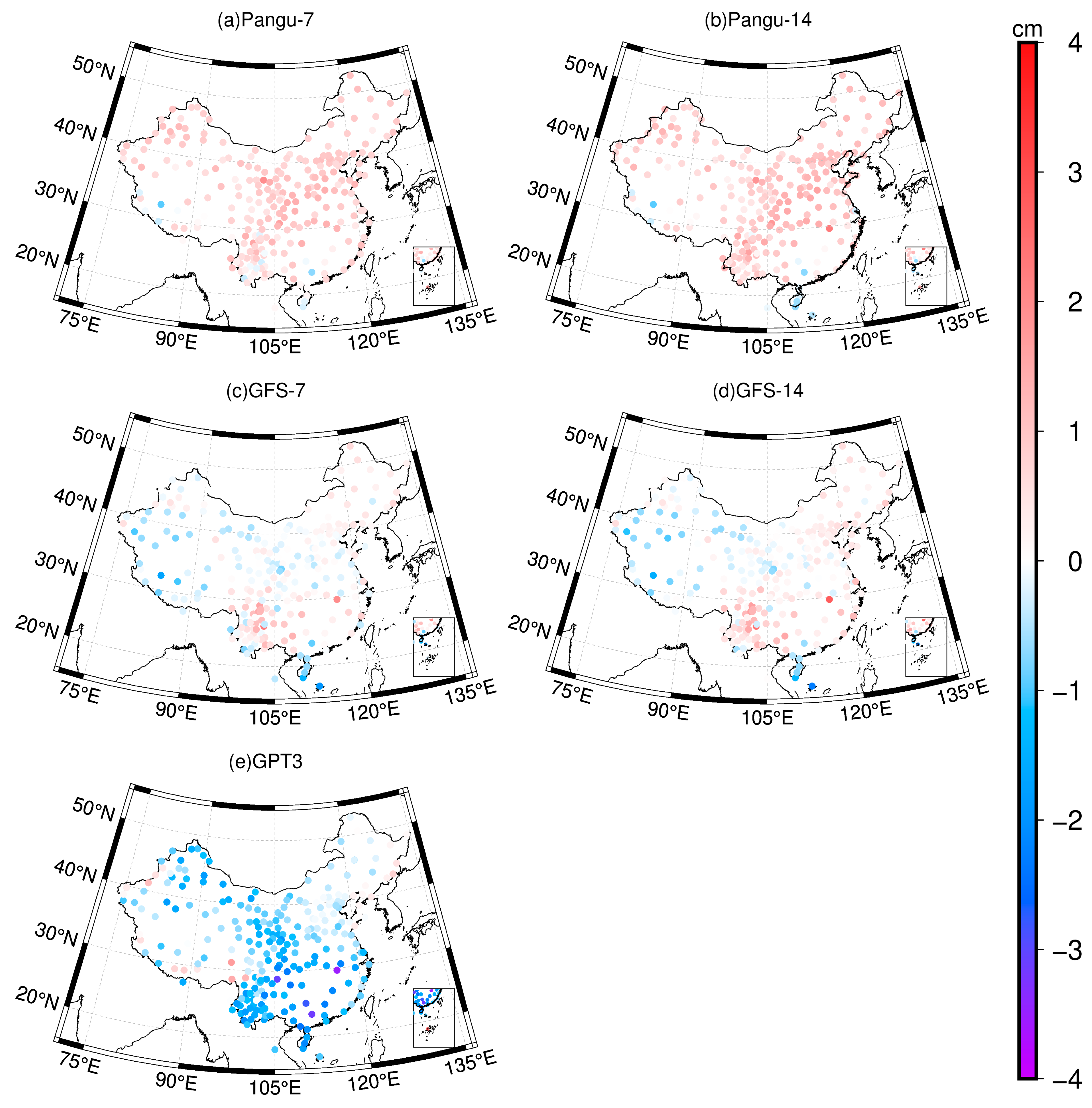
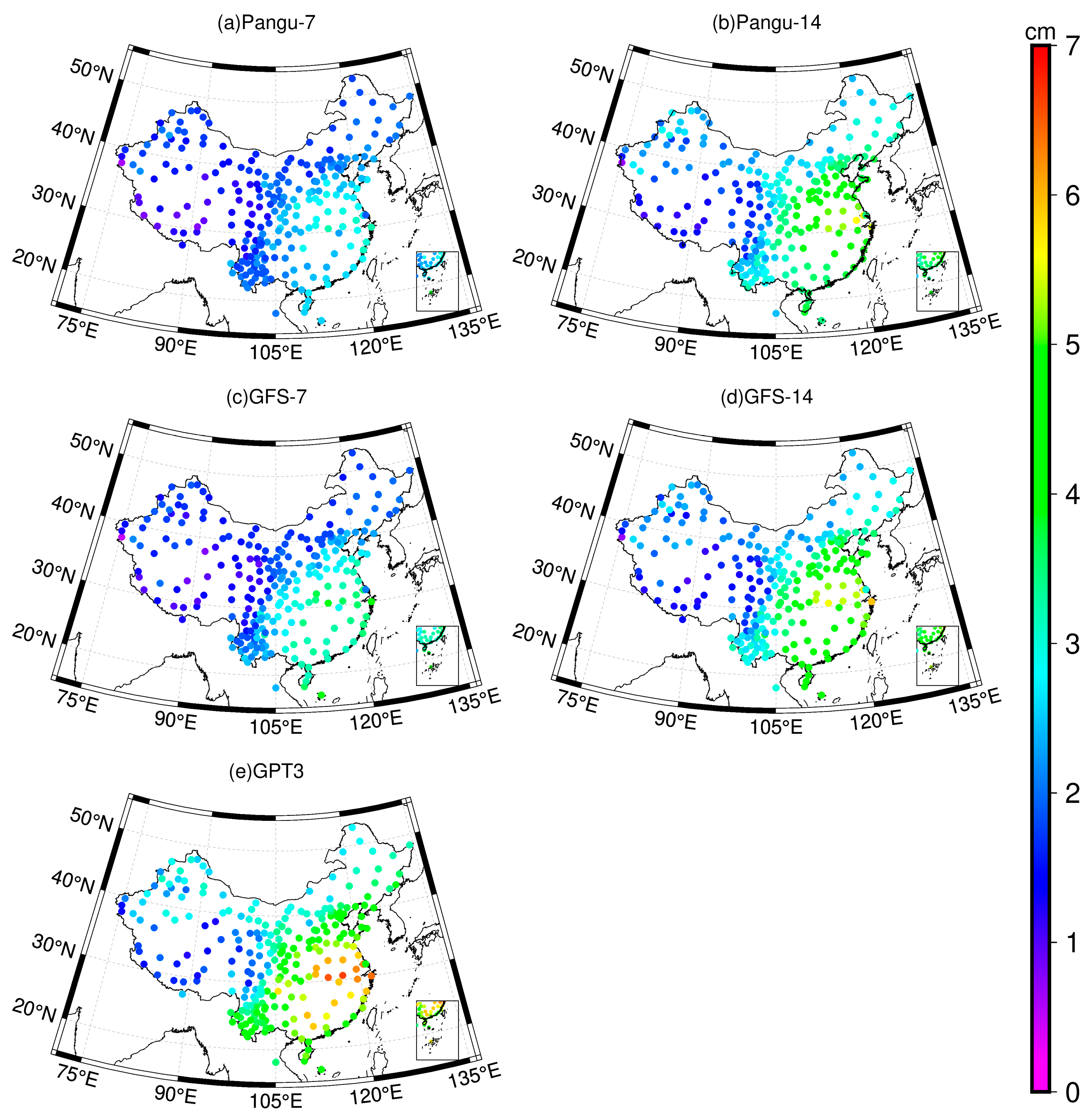
The Pangu-Weather model, the GFS product, and the GPT3 empirical model are validated using hourly ZTD values for each day in 2020 from GNSS stations provided by CMONOC as reference data [26]. The bias and RMSE statistics of different models are summarized in Table 2 and illustrated in Figure 2 and Figure 3.
As shown in Table 2, the GFS product achieves the lowest mean bias under both forecast scales, with values of 0.06 cm and 0.16 cm, compared to the Pangu-Weather model and the GPT3 empirical model. However, its bias fluctuation ranges from −1.95 to 2.32 cm and from −2.29 to 2.78 cm, exceeding those of the Pangu-Weather model, which range from −0.95 to 1.95 cm and from −0.94 to 2.26 cm. Based on the RMSE results, the mean RMSE values of the GFS product are 2.16 cm and 2.98 cm for the two forecast scales, which are higher than those of the Pangu-Weather model (Pangu-7: 1.99 cm and Pangu-14: 2.94 cm) and inconsistent with the performance in terms of mean bias. These results indicate that the positive and negative deviations of the GFS product are relatively unstable, leading to the mutual cancelation of errors and thus a lower mean bias. Overall, the Pangu-Weather model demonstrates higher accuracy in forecasting ZTD over the China region. Meanwhile, both the Pangu-Weather model and the GFS product outperform the GPT3 model in terms of both bias and RMSE statistics.
Figure 2 shows that both forecast scales of the Pangu-Weather model exhibit a significant positive bias over the China region, indicating that the forecasted ZTD values are larger than the GNSS-derived ZTD. The bias distributions of the two forecast scales are similar, although the bias of Pangu-14 is slightly larger. In contrast, the GPT3 empirical model demonstrates a pronounced negative bias across China, particularly with slightly larger absolute bias values at low latitudes. However, the GFS product presents a comparable number of positive and negative biases across the two forecast scales, with most station biases performing better than those of the Pangu-Weather model and the GPT3 empirical model.
In Figure 3, although the GFS product achieves the most favorable bias performance at GNSS stations across China, its RMSE distribution is slightly inferior to that of the Pangu-Weather model, particularly in eastern and southern China, where larger RMSE values are observed. With increasing forecast time, both the Pangu-Weather model and the GFS product exhibit a noticeable increase in RMSE values, especially in regions affected by complex climate conditions and relatively active water vapor, where the impact is more pronounced. Additionally, under longer forecast lead times, the GFS product remains inferior to the Pangu-Weather model in these regions. Notably, the overall RMSE distributions of both the Pangu-Weather model and the GFS product are kept lower than that of the GPT3 empirical model under a 14-day forecast horizon, which indicates that the empirical model is limited in dynamically responding to real-time meteorological variations and results in larger errors.

4.2. Accuracy Analysis of Density Scatter for Four Randomly Selected Stations

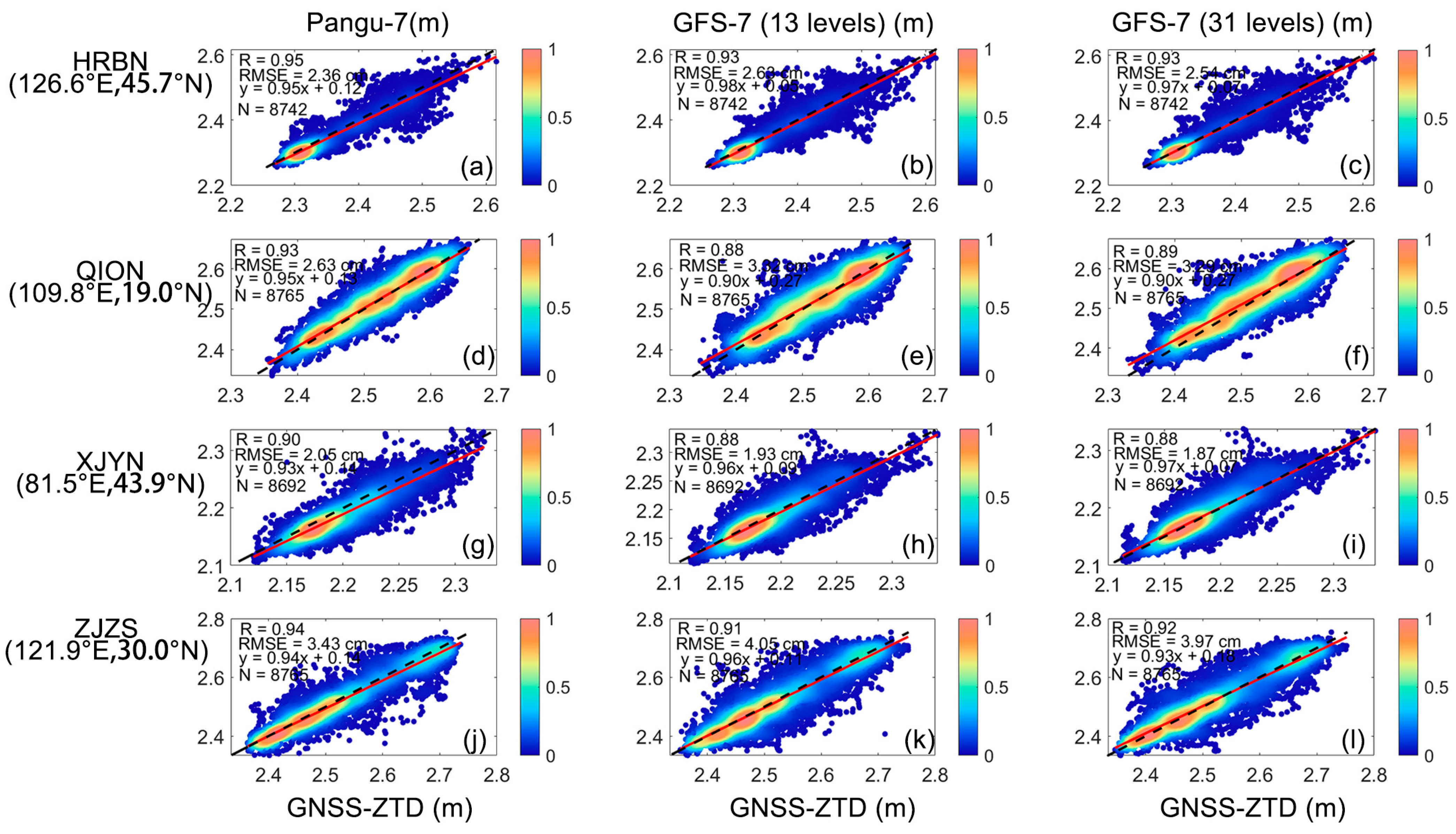
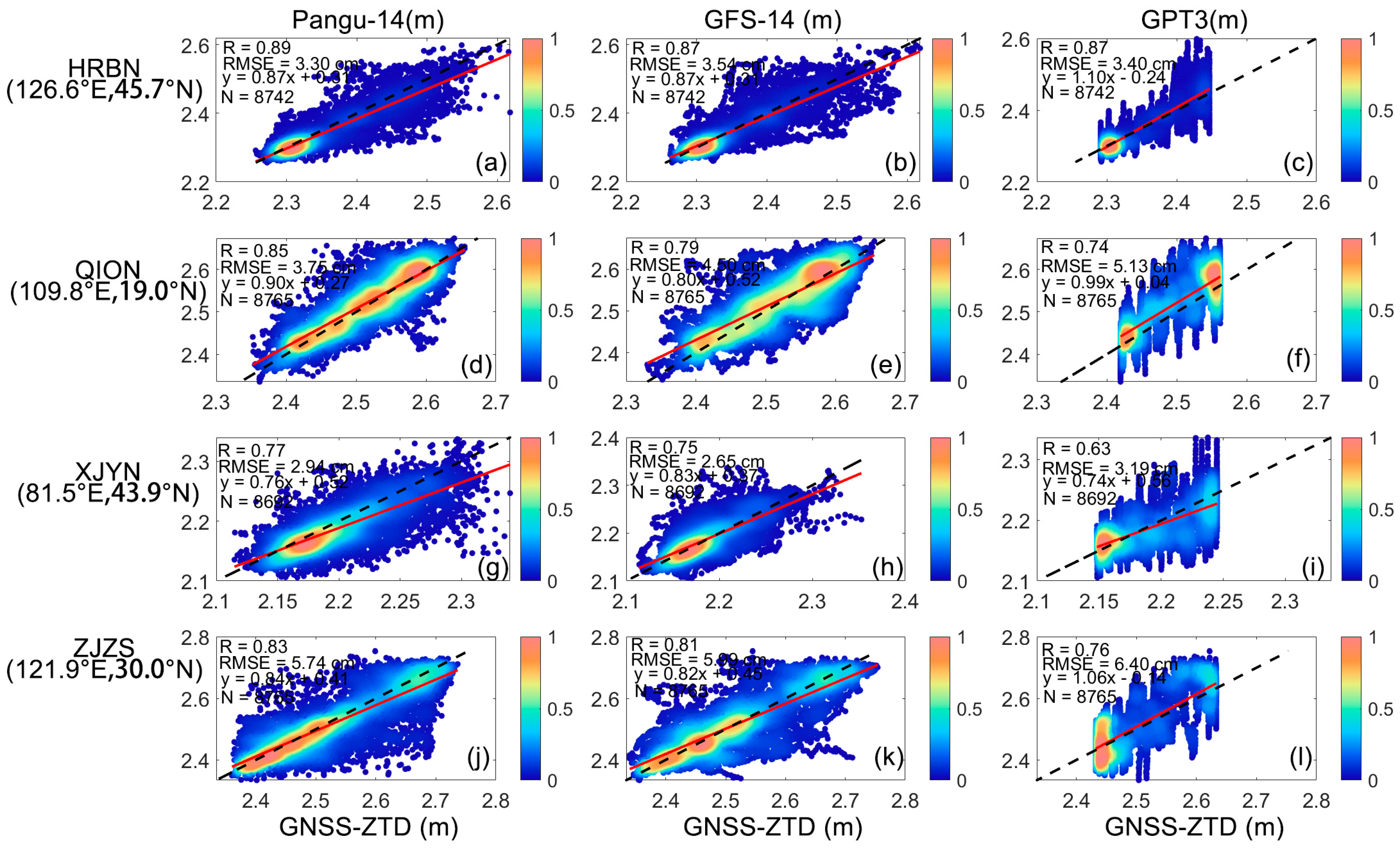
To further investigate the forecasting performance of the Pangu-Weather model, four GNSS stations with relatively complete datasets are randomly selected from the eastern, southern, western, and northern regions. The forecast accuracy is evaluated using the RMSE and the R, and the results are presented in Figure 4 and Figure 5.
As can be seen from Figure 4, when the GFS product is used to calculate ZTD values with the same 13 pressure levels as the Pangu-7 model, the values at the four stations show slightly greater dispersion compared to the results calculated using all pressure levels, with a slightly higher RMSE and a slightly lower R. The correlation coefficients (R) between the Pangu-7 model and GNSS-ZTD all exceed 0.90, which indicates that the Pangu-Weather model has a strong capability to capture the trend of ZTD changes on a 7-day forecast scale. Unfortunately, at the XJYN station, the RMSE values for the Pangu-Weather model are higher than those of the GFS product for both pressure-level resolutions. This may be related to the relatively low water vapor content in the northwest region, where the ZTD is primarily dominated by the hydrostatic tropospheric delay, which is directly related to atmospheric pressure. In comparison, the GFS product provides a finer assimilation and characterization of the pressure field in dry, low-humidity, small-scale areas. In contrast, in the humid southern regions of China, where water vapor content is high and ZTD variability is pronounced, the dominance of ZWD is considered to make the model’s dynamic responsiveness to moisture more crucial. The Pangu-Weather model, built on the Transformer architecture, is better suited for capturing large-scale meteorological patterns and is shown to possess a stronger capability in learning nonlinear features in complex humidity fields.
In Figure 5, with increasing forecast time, both models exhibit consistent performance between the 14-day and 7-day forecast scales at the four stations. The Pangu-7 model demonstrates the highest correlation coefficients compared to the other two models. However, the Pangu-Weather model still presents higher RMSE values than the GFS product at the XJYN station, as previously explained. In contrast, the scatter distribution of the GPT3 model is relatively dispersed across the four stations, while more scatter points of the AI-based Pangu-14 based on the Transformer architecture align closely with the 1:1 line and indicate better forecast performance.

4.3. Accuracy Analysis of Different Latitude Belts and Different Height Ranges

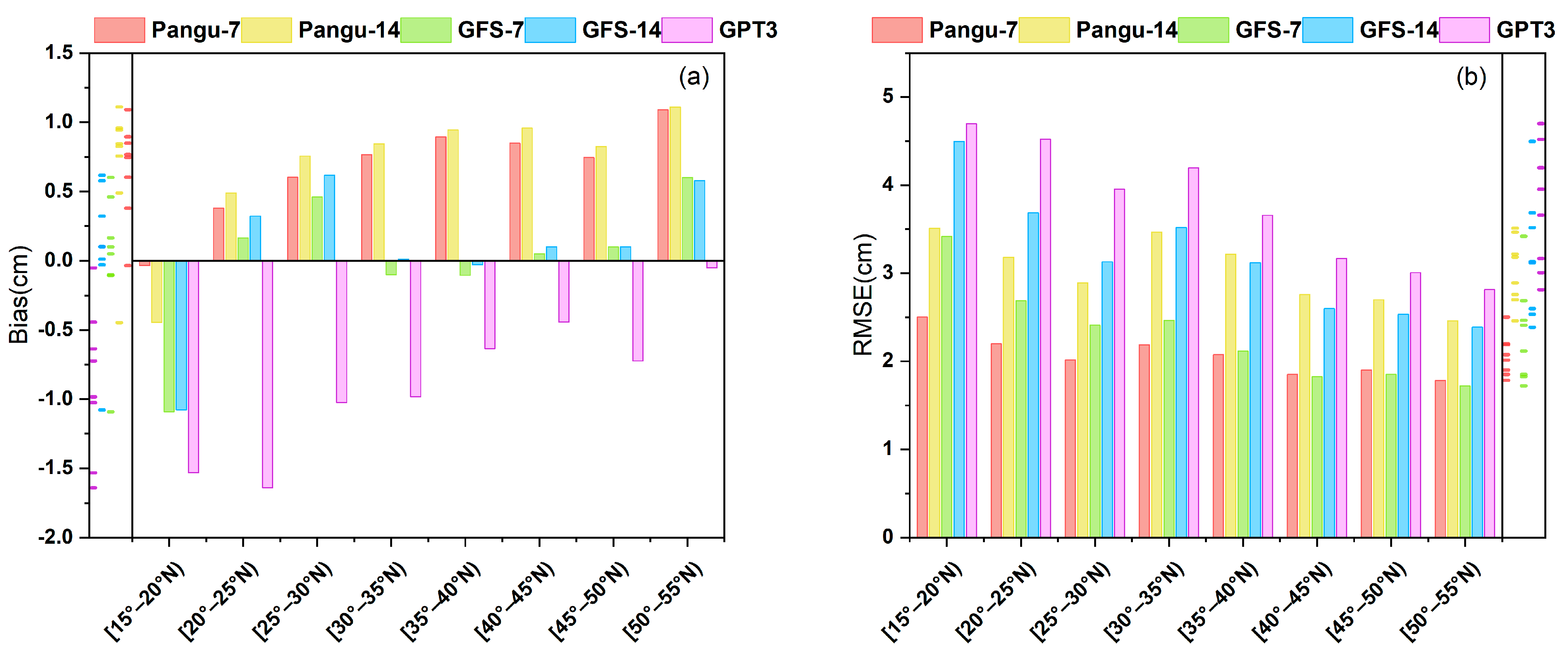
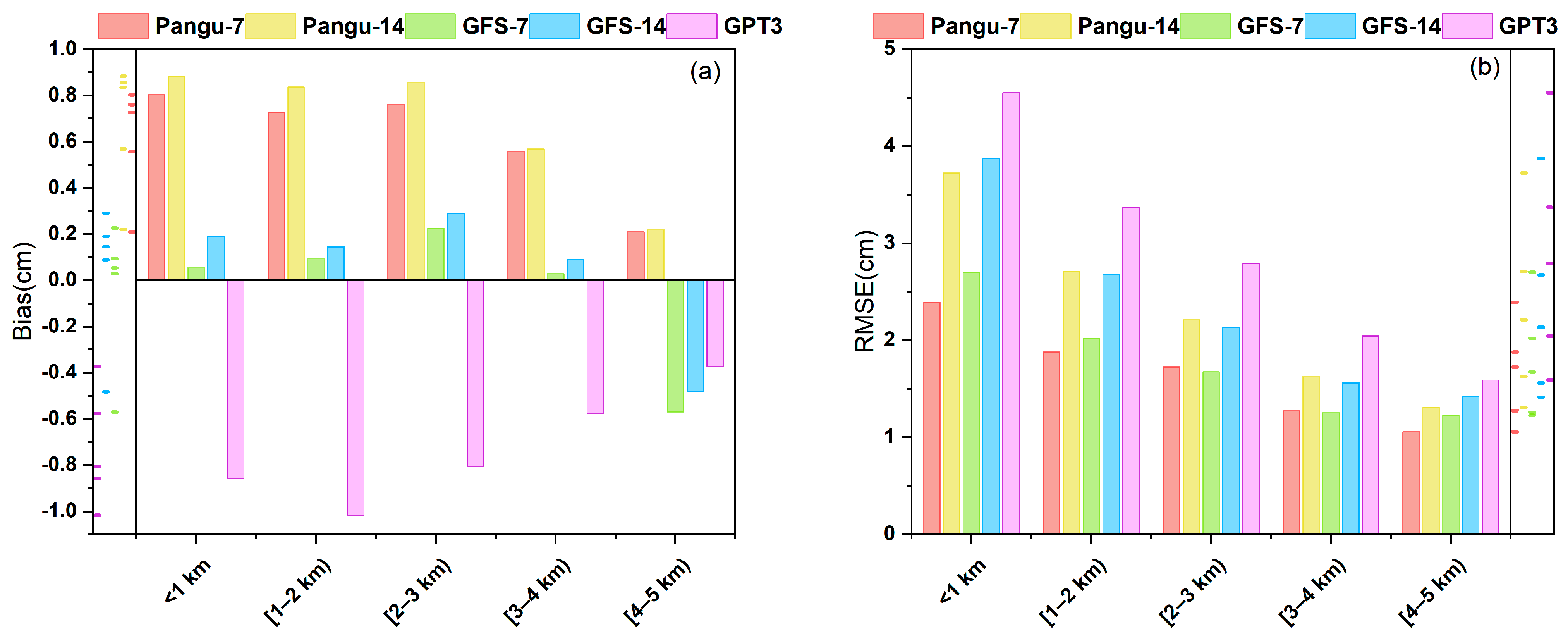
Previous studies have demonstrated that ZTD is significantly correlated with both elevation and latitude [52,53,54]. To further analyze the distribution characteristics of bias and RMSE for the three models with respect to latitude and elevation, the 250 GNSS stations are categorized at 5° latitude intervals and 1 km elevation intervals. The results are presented in Figure 6 and Figure 7.
As shown in Figure 6, across different latitude bands and forecast time scales, the Pangu-Weather model outperforms the GFS product in terms of bias only within the 15–20°N latitude band. In contrast, the GFS product achieves mean bias values close to 0 cm in the mid- and high-latitude regions. The GPT3 empirical model exhibits the lowest mean bias within the 50–55°N latitude band. The Pangu-Weather model demonstrates significantly lower mean RMSE values than the GFS product in low-latitude regions, particularly within the 15–20°N latitude band, where the 14-day forecast RMSE of the Pangu-Weather model approaches that of the GFS product at the 7-day forecast scale. However, within the 20–40°N latitude band, the Pangu-Weather model achieves lower RMSE values compared to the GFS product, although its poorer bias performance can be attributed to the reasons previously discussed. In the 40–55°N latitude band, the RMSE performance of the Pangu-Weather model is slightly inferior to that of the GFS product but remains superior to that of the GPT3 empirical model overall.
In Figure 7, the Pangu-Weather model achieves the best mean bias only at stations located at 4–5 km elevations, while the GFS product exhibits the optimal mean bias at stations below 4 km. The GPT3 empirical model continues to show the poorest ZTD forecast performance at these stations, with significantly larger negative bias values. From the RMSE, it is observed that the Pangu-Weather model provides the best forecast accuracy at stations below 1 km and between 4 and 5 km. In addition, Pangu-7 maintains the lowest RMSE at stations between 1 and 2 km, whereas Pangu-14 begins to perform slightly worse than the GFS product in this range. However, at stations located between 2 and 4 km, slightly inferior forecast accuracy is shown by the Pangu-Weather model compared to the GFS product. This is attributed to the use of only 13 pressure levels in the Pangu-Weather model, leading to lower vertical interpolation precision compared to the GFS product, which uses 31 pressure levels.

4.4. Accuracy Analysis of Different Months

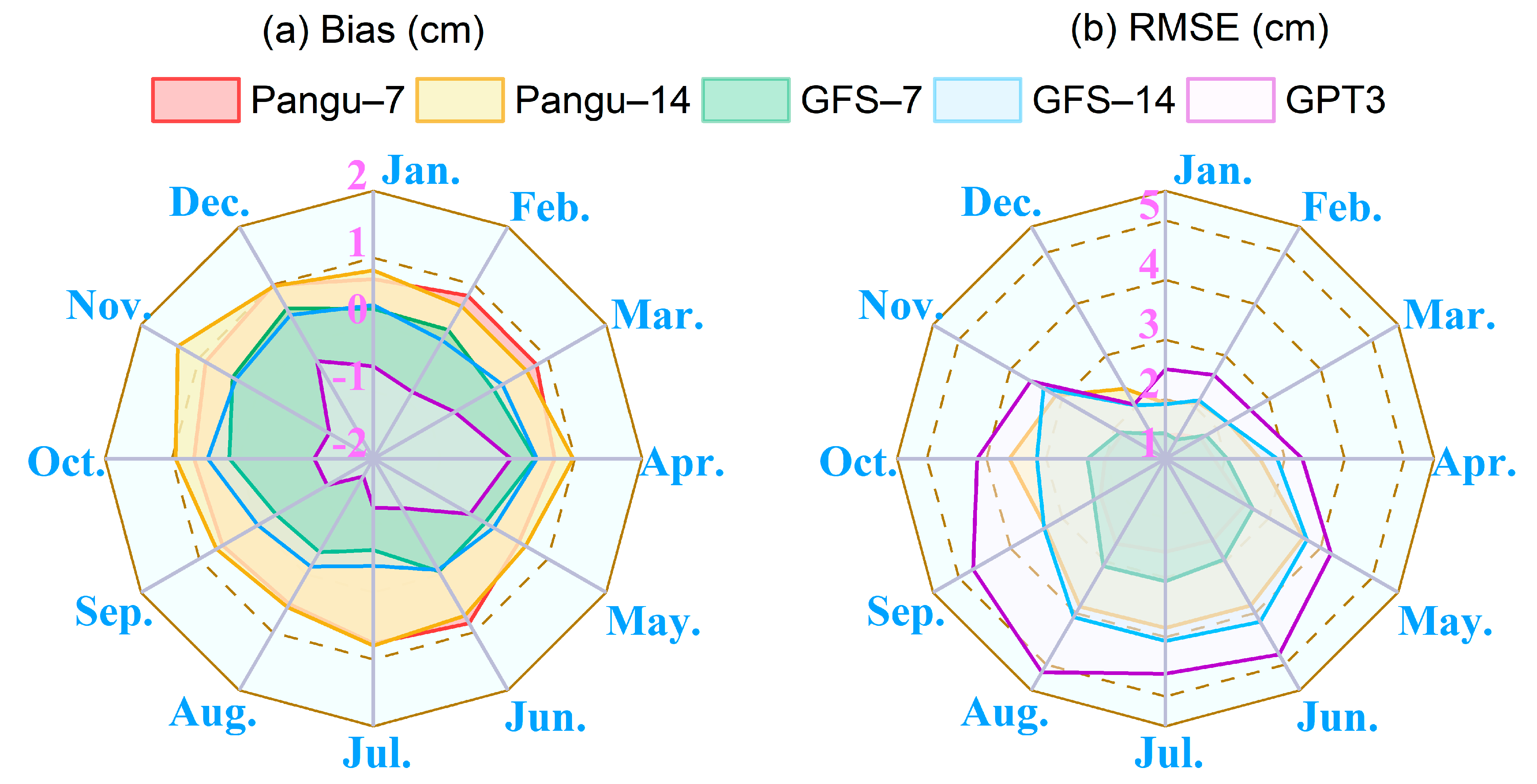
To analyze the monthly variations in bias and RMSE in ZTD calculated using the three models, the bias and RMSE values at 250 GNSS stations are statistically meant by month. The results are shown in Figure 8.
As illustrated in Figure 8, the Pangu-Weather model exhibits a consistently positive monthly mean Bias under both forecast time scales, with a relatively stable fluctuation range remaining within approximately 1 cm throughout the year. In contrast, the GFS product achieves the lowest monthly mean Bias across all months, with values oscillating around 0 cm. The GPT3 empirical model shows a persistent negative Bias throughout the year. Regarding RMSE performance, all five models display a distinct seasonal variation, with RMSE values peaking during the summer months. This increase is likely associated with the climatic characteristics of summer in China, which is dominated by a monsoonal regime [55,56]. Influenced by warm and humid oceanic air masses, atmospheric parameters such as water vapor become highly active and variable during this period. This poses challenges for numerical weather forecast models, including Pangu-Weather and GFS, in accurately capturing rapid and complex ZTD variations. Nevertheless, both models still maintain a clear advantage over the GPT3 empirical model in terms of accuracy. It is noteworthy that under the 7-day forecast time scale, the Pangu-Weather model consistently outperforms the GFS product in terms of monthly mean RMSE throughout the year. Under the 14-day forecast time scale, the Pangu-Weather model only exhibits slightly higher RMSE values than the GFS product in October and December. Overall, the Pangu-Weather model demonstrates strong year-round stability and minimal error fluctuation, highlighting its robustness and adaptability in ZTD forecasting across different temporal and climatic conditions.

4.5. Accuracy Evaluation of RMSE in 7-Day and 14-Day ZTD Forecasting

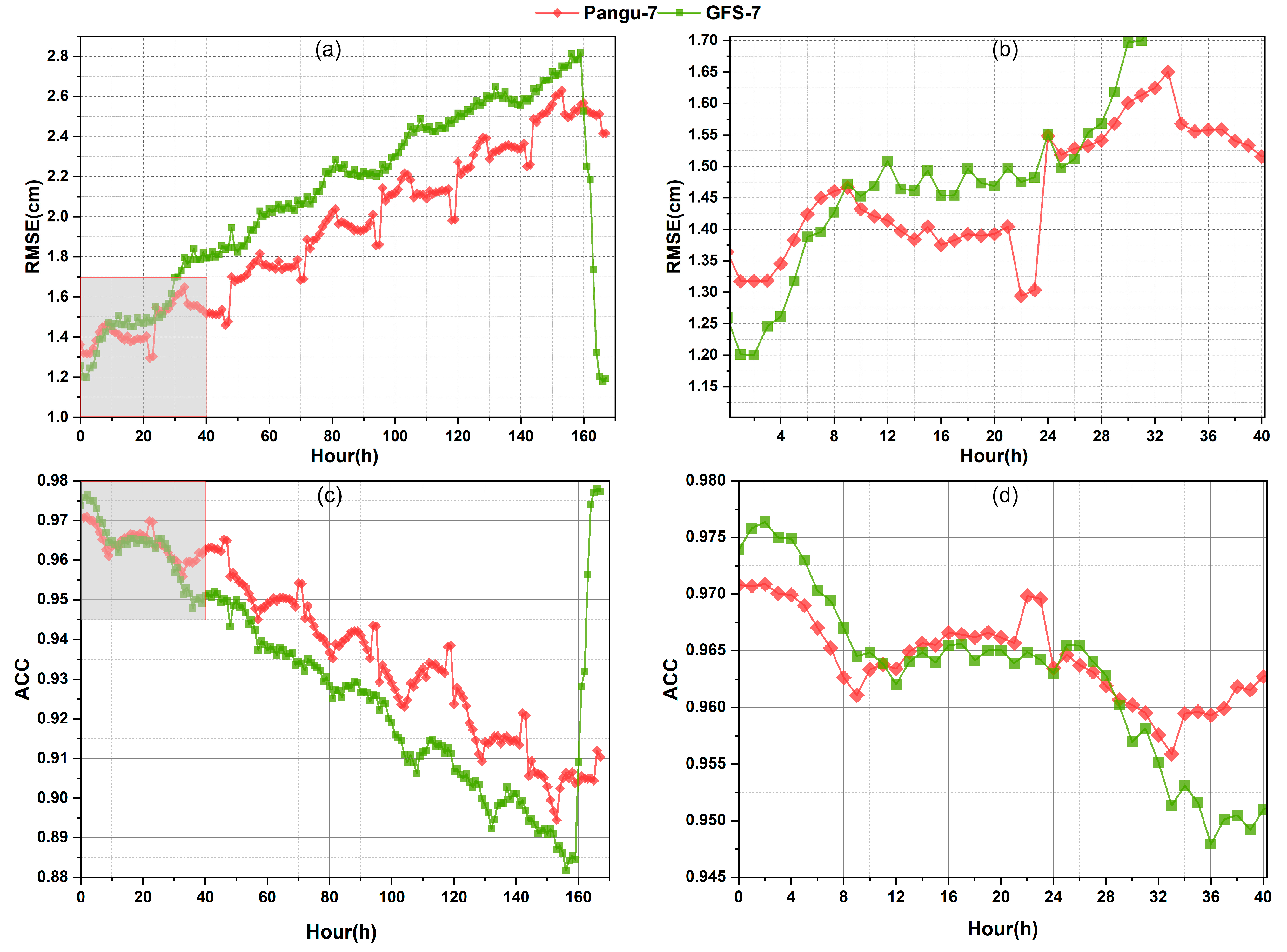
To more clearly illustrate the variation characteristics of the hourly RMSE values for the Pangu-Weather model and the GFS product over 7-day and 14-day forecasts, the forecasted values are separated over each 7-day and 14-day period. The corresponding time series plots are presented in Figure 9 and Figure 10.
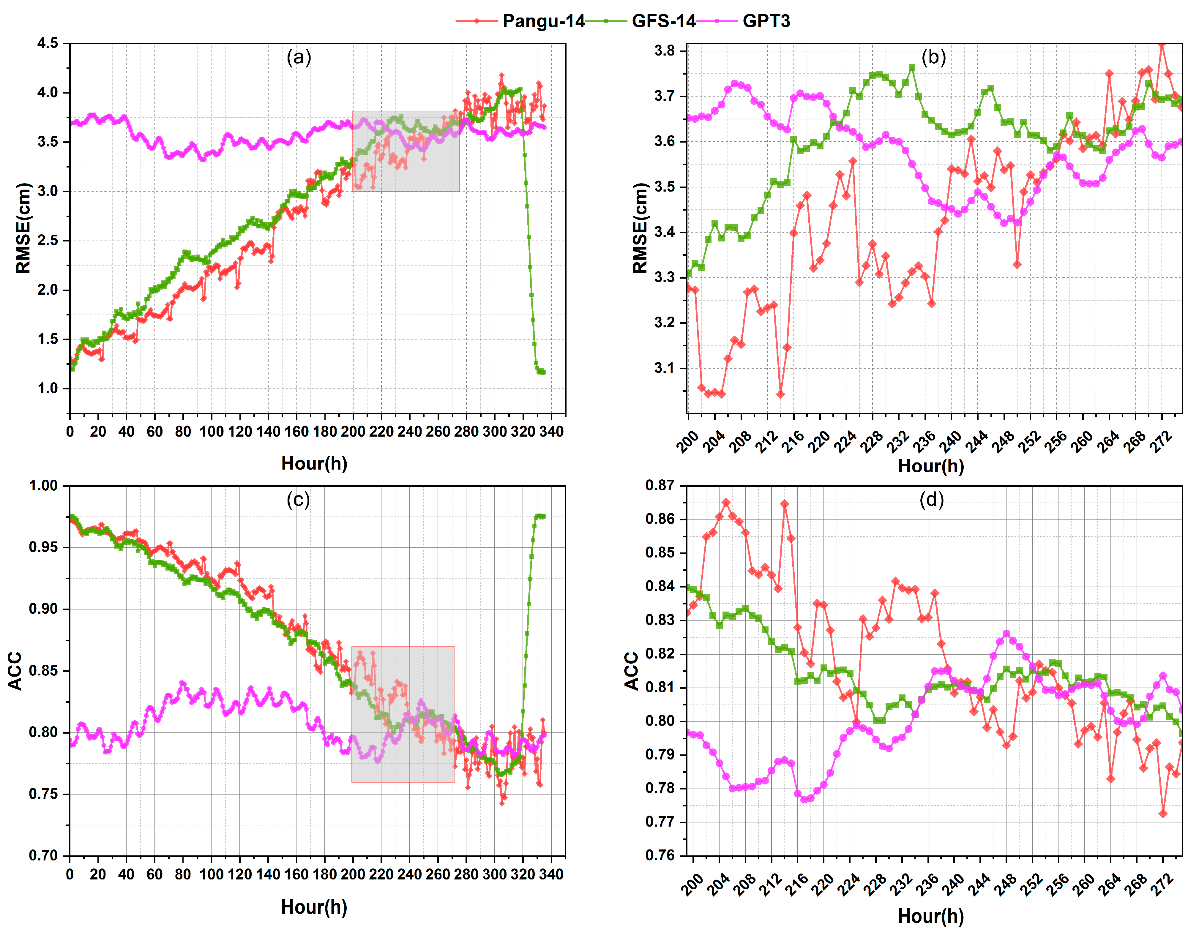
As shown in Figure 9a,b, the RMSE values of both the Pangu-Weather model and the GFS product exhibit a continuous increase with the extension of forecast time. Due to the Pangu-Weather model’s employment of a hierarchical temporal aggregation strategy for forecasting, its RMSE experiences a periodic increase after every 24 h cycle. In contrast, the GFS product reveals a greater tendency toward error accumulation over longer forecast ranges, resulting in a steeper RMSE growth rate. Notably, abrupt RMSE drops observed between hours 159 to 163 and 319 to 335 are attributed to the reinitialization of the GFS product’s initial fields. During the first 9 forecast hours, the GFS product maintains the lowest RMSE due to its finer vertical pressure level resolution. This allows it to more accurately capture the vertical gradient changes in key meteorological elements, such as temperature inversions and humidity stratification, leading to more precise short-term ZTD predictions. In contrast, the Pangu-Weather model’s use of only 13 pressure levels results in a coarse resolution, which is prone to physical quantity interpolation errors due to insufficient vertical stratification when handling complex terrain or weather systems with intense vertical movement. This type of error is quickly magnified, particularly in short-term forecasts. Beyond the 9 h mark, the Pangu-Weather model gradually surpasses the GFS product in forecast accuracy. Figure 9c,d show hourly mean ACC statistics, revealing a trend opposite to that of the RMSE values, as the ACC decreases with increasing forecast time. The decline is more pronounced for the GFS product, whereas the Pangu-Weather model exhibits a periodic and slower decrease. However, differing from the RMSE behavior in the early forecast period, higher ACC values than those of the GFS product are achieved by the Pangu-Weather model only after the 12th forecast hour.
From Figure 10, temporal analysis over the 14-day forecast horizon reveals that the Pangu-Weather model and GFS product do not consistently outperform the GPT3 empirical model throughout the forecast period. Specifically, the RMSE values of the two models became slightly higher than those of the GPT-3 model after 240 h and 223 h, respectively, while their ACC values began to fall below those of the GPT-3 model after 240 h and 232 h, respectively. These results indicate that while the GFS product shows superior performance in very short-range forecasts, the deep neural network-driven Pangu-Weather model demonstrates more stable accuracy over longer forecast periods. Compared to the conventional GFS numerical weather prediction product, the Pangu-Weather model shows greater adaptability to complex meteorological conditions.

4.6. Accuracy Analysis of Models Under Complex Weather Conditions

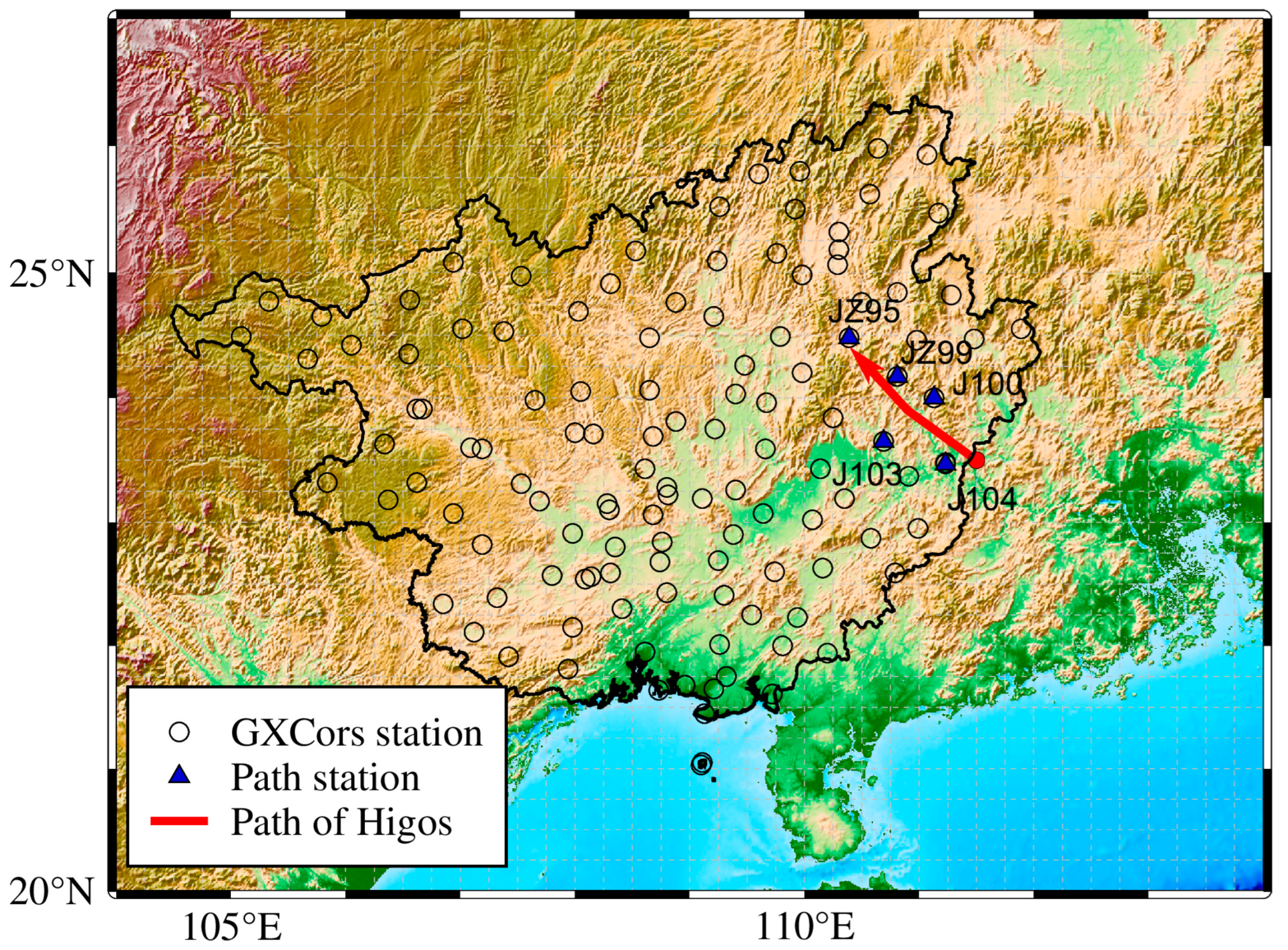
Strong convection and other extreme weather events are considered to be the main challenges for the accurate estimation of tropospheric delay. Typhoon Higos, the seventh named storm of 2020 (international ID: 2007), was generated over the South China Sea at 06:00 UTC on 11 August, and gradually intensified before making landfall along the coast of Zhuhai, Guangdong Province, at 02:30 UTC on 19 August. After landfall, Higos continued its northwestward movement, entering Guangxi at 17:00 UTC on 19 August, after which it gradually weakened and eventually dissipated over Guangxi at 06:00 UTC on 20 August. Under the influence of Higos, sustained heavy rainfall and strong water vapor transport are observed in the Guangxi region, accompanied by a significant release of energy. For this study, five GXCORS stations located along the typhoon’s path are selected to comprehensively evaluate the applicability of the Pangu-Weather model under the complex atmospheric conditions induced by Higos. The Track of Typhoon Higos and the distribution of the GXCORS stations are shown in Figure 11.
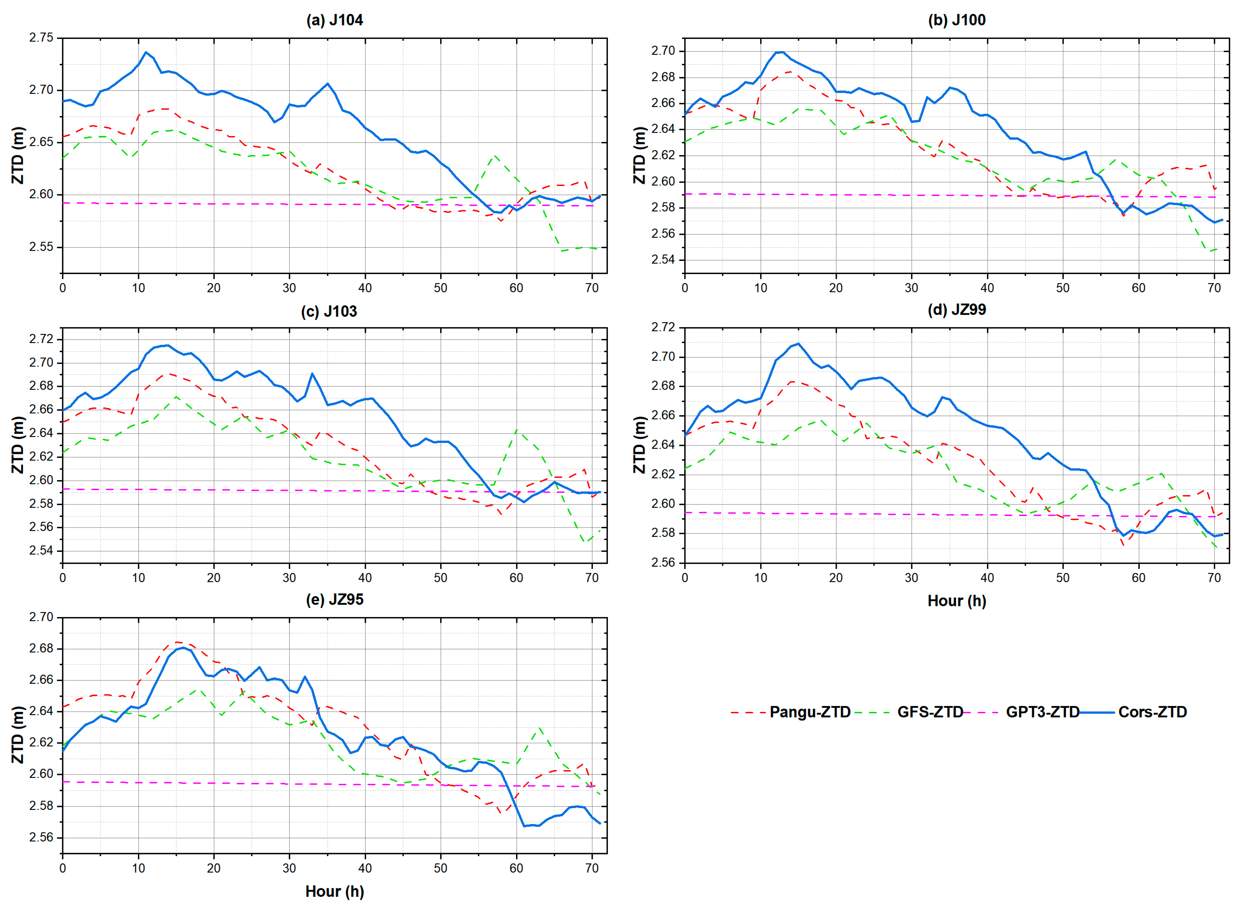
Table 3 presents the accuracy statistics of the Pangu-Weather model and the GFS product at five GXCORS stations along the track of Typhoon Higos from 00:00 UTC on 19 August to 23:00 UTC on 21 August 2020. Figure 12 illustrates the ZTD time series predicted by the Pangu-Weather model, the GFS product and the GPT3 empirical model at these five stations.
As shown in Table 3, during the extreme weather conditions of Typhoon Higos, the ZTD predictions from the Pangu-Weather model, which has the same temporal forecast scale, exhibit significantly better performance in terms of RMSE and Bias compared to the ZTD predictions from the GFS product across the five GXCORS stations. As illustrated in the ZTD time series during the extreme weather event of Typhoon Higos in Figure 12, the Pangu-Weather model’s predictions are closer to the CORS-derived ZTD at these stations, particularly in reproducing the arrival of the peak on 19 August and the subsequent gradual downward trend. In contrast, the GFS product generally underestimates the ZTD values, especially during the peak water vapor period (early 19 August), and shows greater fluctuations, deviating from the trend of the actual observations. The ZTD values predicted by the GPT3 empirical model are represented as a smooth curve, and the sharp fluctuations induced by extreme weather cannot be captured. In summary, the ZTD prediction accuracy of the Pangu-Weather model is superior to that of the GFS product for the Guangxi region during Typhoon Higos, and it performs more stably, especially during periods of rapid water vapor change. The GFS and GPT3 models exhibit systematic biases and fluctuations during the peak period, which makes it difficult to accurately reflect the water vapor anomalies brought by the typhoon.

5. Conclusions

The performance of tropospheric delay is crucial for ensuring high-precision positioning, navigation, and timing applications. As is well known, the VMF3_FC product, provided by the IFS of ECMWF, is a widely used tropospheric delay product that already offers next-day predictions. However, due to the complexity of its numerical prediction model and the limited forecast ability, generating a 10-day forecast typically requires several hours of computation on supercomputers. In contrast, the emergence of artificial intelligence (AI)-driven weather models, such as Pangu-Weather, has achieved higher forecast accuracy and significantly faster computational speeds, opening new opportunities for real-time, high-accuracy, and high-resolution tropospheric delay estimation.
Therefore, a Pangu-Weather ensemble forecasting approach based on multiple initial conditions is proposed to obtain hourly resolution estimates of tropospheric delay. The performance of the proposed method is validated with the data from 250 GNSS stations across China in year of 2020, and a comprehensive analysis is conducted with the traditional NWP model GFS and the GPT3 empirical model. The findings show that the Pangu-Weather model exhibits strong performance under both forecast speeds compared to the traditional GFS product, particularly in southern China. However, the Pangu-Weather model’s ability to capture data is found to be weaker than the GFS product with the same 13 pressure levels in dry, low-humidity, small-scale regions (e.g., at the XJYN station). Furthermore, because the Pangu-Weather model uses only 13 pressure levels, its forecast performance at stations between 2 and 4 km and for short-term forecasts (<9 h) is slightly inferior to that of the GFS model which uses 31 pressure levels. Nevertheless, the Pangu-Weather model, which is based on deep learning algorithms, is found to exhibit a smaller cumulative error trend and to maintain more stable forecast accuracy over longer prediction horizons. The model is also considered to have stronger adaptability to complex meteorological conditions, and its performance advantage is especially evident during periods of rapid water vapor change in extreme weather events. In future work, efforts will be focused on integrating multiple AI-driven weather models and utilizing initial fields from more diverse sources to generate an increased number of forecast members. Concurrently, AI-based meteorological frameworks will also be used to improve global ZTD estimation, while also advancing the more critical estimation of slant path tropospheric delay.

Author Contributions

Conceptualization, S.L., B.S. and H.B.; Data curation, S.L., H.B., L.H. and Q.A.; Formal analysis, S.L., B.S. and H.B.; Funding acquisition, B.Z.; Investigation, Q.A.; Methodology, S.L., B.S. and H.B.; Project administration, B.Z.; Resources, B.S.; Software, B.S. and L.H.; Supervision, L.H.; Validation, S.L. and L.H.; Visualization, Q.A.; Writing—original draft, S.L., B.S. and H.B.; Writing—review & editing, S.L., H.B. and B.Z. All authors have read and agreed to the published version of the manuscript.

Funding

This research was funded by the Natural Science Foundation of Hubei Province (No. 2023AFB435); State Key Laboratory of Precision Geodesy, Innovation Academy for Precision Measurement Science and Technology (No. SKLGED2024-3-3).

Data Availability Statement

The ERA5 data are available at https://cds.climate.copernicus.eu/datasets (accessed on 20 March 2025). The GFS data are obtained from https://www.ncei.noaa.gov/products/weather-climate-models/global-forecast (accessed on 20 March 2025). The Pangu-Weather model code is obtained from https://github.com/198808xc/Pangu-Weather (accessed on 20 March 2025).

Acknowledgments

The authors thank CMONOC (Crustal Movement Observation Network of China) for providing GNSS data, ECMWF (European Centre for Medium-Range Weather Forecasts) for providing the ERA5 grid data, NOAA (National Oceanic and Atmospheric Administration) for providing the GFS data and Huawei Cloud for providing the Pangu-Weather model code in this study.

Conflicts of Interest

Author Shuangping Li was employed by the company Changjiang Spatial Information Technology Engineering Co., Ltd. The remaining authors declare that the research was conducted in the absence of any commercial or financial relationships that could be construed as a potential conflict of interest.

Abbreviations

The following abbreviations are used in this manuscript:
GNSSGlobal Navigation Satellite Systems
ZTDZenith Total Delay
PWVPrecipitable Water Vapor
GPT3Global Pressure and Temperature 3
ECMWFEuropean Centre for Medium-Range Weather Forecasts
NWPNumerical Weather Prediction
GFSGlobal Forecast System
IFSIntegrated Forecasting System
AIArtificial Intelligence
NCEPNational Centers for Environmental Prediction
CMONOCCrustal Movement Observation Network of China

References

  1. Dousa, J.; Elias, M. An improved model for calculating tropospheric wet delay. Geophys. Res. Lett. 2014, 41, 4389–4397. [Google Scholar] [CrossRef]
  2. Huang, L.; Zhu, G.; Liu, L.; Chen, H.; Jiang, W. A global grid model for the correction of the vertical zenith total delay based on a sliding window algorithm. Gps Solut. 2021, 25, 98. [Google Scholar] [CrossRef]
  3. Li, H.; Zhu, G.; Kang, Q.; Huang, L.; Wang, H. A global zenith tropospheric delay model with ERA5 and GNSS-based ZTD difference correction. Gps Solut. 2023, 27, 154. [Google Scholar] [CrossRef]
  4. Huang, L.; Pan, A.; Chen, F.; Guo, F.; Li, H.; Liu, L. A novel global grid model for soil moisture retrieval considering geographical disparity in spaceborne GNSS-R. Satell. Navig. 2024, 5, 29. [Google Scholar] [CrossRef]
  5. Li, J.; Zhang, Q.; Liu, L.; Yao, Y.; Huang, L.; Chen, F.; Zhou, L.; Zhang, B. A refined zenith tropospheric delay model for Mainland China based on the global pressure and temperature 3 (GPT3) model and random forest. Gps Solut. 2023, 27, 172. [Google Scholar] [CrossRef]
  6. Li, S.; Jiang, N.; Xu, T.; Xu, Y.; Yang, H.; Zhang, Z.; Guo, A.; Wu, Y. A precipitation forecast model with a neural network and improved GPT3 model for Japan. Gps Solut. 2023, 27, 186. [Google Scholar] [CrossRef]
  7. Yuan, P.; Blewitt, G.; Kreemer, C.; Hammond, W.C.; Argus, D.; Yin, X.; Van Malderen, R.; Mayer, M.; Jiang, W.; Awange, J.; et al. An enhanced integrated water vapour dataset from more than 10 000 global ground-based GPS stations in 2020. Earth Syst. Sci. Data 2023, 15, 723–743. [Google Scholar] [CrossRef]
  8. Xiong, L.; Huang, L.; Mo, Z.; Chen, X.; Yang, Y.; Xie, S.; Li, J.; Liu, L. Evolution of GNSS-Derived Precipitable Water Vapor and Its Driving Factors During the “Dragon Boat Water” Rainfall Event in Guangxi, China. IEEE J. Sel. Top. Appl. Earth Obs. Remote Sens. 2025, 18, 14308–14323. [Google Scholar] [CrossRef]
  9. Huang, L.; Zheng, Z.; Zhu, G.; Bi, H.; Li, H.; Liu, L. A Novel Method for Forecasting Global High-Resolution Precipitable Water Vapor with The Pangu-Weather System. IEEE J. Sel. Top. Appl. Earth Obs. Remote Sens. 2025, 18, 14843–14854. [Google Scholar] [CrossRef]
  10. Xu, C.; Liu, C.; Yao, Y.; Wang, Q.; Wang, X. Tibetan zenith wet delay model with refined vertical correction. J. Geod. 2023, 97, 31. [Google Scholar] [CrossRef]
  11. Yang, F.; Guo, J.; Meng, X.; Li, J.; Zou, J.; Xu, Y. Establishment and assessment of a zenith wet delay (ZWD) augmentation model. Gps Solut. 2021, 25, 148. [Google Scholar] [CrossRef]
  12. Zhao, X.; Niu, Q.; Chi, Q.; Chen, J.; Liu, C. A new LSTM-based model to determine the atmospheric weighted mean temperature in GNSS PWV retrieval. Gps Solut. 2024, 28, 74. [Google Scholar] [CrossRef]
  13. Li, J.; Li, F.; Liu, L.; Yao, Y.; Huang, L.; Wang, Y. A weighted mean temperature forecast model based on fused data and generalized regression neural network and its impact on GNSS-Based precipitable water vapor estimation. IEEE Trans. Geosci. Remote 2024, 62, 4101914. [Google Scholar] [CrossRef]
  14. Huang, L.; Lu, D.; Chen, F.; Zhang, H.; Zhu, G.; Liu, L. A Deep Learning-Based Approach for Directly Retrieving GNSS Precipitable Water Vapor and Its Application in Typhoon Monitoring. IEEE Trans. Geosci. Remote 2024, 62, 4111712. [Google Scholar] [CrossRef]
  15. Hopfield, H.S. Two-quartic tropospheric refractivity profile for correcting satellite data. J. Geophys. Res. 1969, 74, 4487–4499. [Google Scholar] [CrossRef]
  16. Saastamoinen, J. Atmospheric correction for the troposphere and stratosphere in radio ranging satellites. Use Artif. Satell. Geod. 1972, 15, 247–251. [Google Scholar] [CrossRef]
  17. Black, H.D. An easily implemented algorithm for the tropospheric range correction. J. Geophys. Res. 1978, 83, 1825–1828. [Google Scholar] [CrossRef]
  18. Askne, J.; Nordius, H. Estimation of tropospheric delay for microwaves from surface weather data. Radio. Sci. 1987, 22, 379–386. [Google Scholar] [CrossRef]
  19. Huang, L.; Jiang, W.; Liu, L.; Chen, H.; Ye, S. A new global grid model for the determination of atmospheric weighted mean temperature in GPS precipitable water vapor. J. Geod. 2019, 93, 159–176. [Google Scholar] [CrossRef]
  20. Ding, M. A neural network model for predicting weighted mean temperature. J. Geod. 2018, 92, 1187–1198. [Google Scholar] [CrossRef]
  21. Zhang, H.; Yuan, Y.; Li, W.; Zhang, B.; Ou, J. A grid-based tropospheric product for China using a GNSS network. J. Geod. 2018, 92, 765–777. [Google Scholar] [CrossRef]
  22. Leandro, R.; Santos, M.; Langley, R.B. UNB neutral atmosphere models: Development and performance. In Proceedings of the 2006 National Technical Meeting of the Institute of Navigation, Monterey, CA, USA, 18–20 January 2006. [Google Scholar]
  23. Leandro, R.F.; Langley, R.B.; Santos, M.C. UNB3m_pack: A neutral atmosphere delay package for radiometric space techniques. Gps Solut. 2008, 12, 65–70. [Google Scholar] [CrossRef]
  24. Lagler, K.; Schindelegger, M.; Böhm, J.; Krásná, H.; Nilsson, T. GPT2: Empirical slant delay model for radio space geodetic techniques. Geophys. Res. Lett. 2013, 40, 1069–1073. [Google Scholar] [CrossRef]
  25. Lan, S.; Zhang, L.; Chen, X.; Yang, Y.; Xiong, S.; Tang, Y.; Huang, L.; Li, X. A novel model for the estimation of water vapor pressure and temperature considering diurnal variations in China. Adv. Space Res. 2025, 75, 515–529. [Google Scholar] [CrossRef]
  26. Landskron, D.; Böhm, J. VMF3/GPT3: Refined discrete and empirical troposphere mapping functions. J. Geod. 2018, 92, 349–360. [Google Scholar] [CrossRef]
  27. Yang, F.; Guo, J.; Zhang, C.; Li, Y.; Li, J. A regional Zenith Tropospheric Delay (ZTD) model based on GPT3 and ANN. Remote Sens. 2021, 13, 838. [Google Scholar] [CrossRef]
  28. Zhao, Q.; Su, J.; Xu, C.; Yao, Y.; Zhang, X.; Wu, J. High-Precision ZTD model of altitude-related correction. IEEE J. Sel. Top. Appl. Earth Obs. Remote Sens. 2023, 16, 609–621. [Google Scholar] [CrossRef]
  29. Zhu, G.; Huang, L.; Yang, Y.; Li, J.; Zhou, L.; Liu, L. Refining the ERA5-based global model for vertical adjustment of zenith tropospheric delay. Satell. Navig. 2022, 3, 27. [Google Scholar] [CrossRef]
  30. Huang, L.; Zhu, G.; Peng, H.; Liu, L.; Ren, C.; Jiang, W. An improved global grid model for calibrating zenith tropospheric delay for GNSS applications. Gps Solut. 2022, 27, 17. [Google Scholar] [CrossRef]
  31. Huang, L.; Lan, S.; Zhu, G.; Chen, F.; Li, J.; Liu, L. A global grid model for the estimation of zenith tropospheric delay considering the variations at different altitudes. Geosci. Model. Dev. 2023, 16, 7223–7235. [Google Scholar] [CrossRef]
  32. Wilgan, K.; Hadas, T.; Hordyniec, P.; Bosy, J. Real-time precise point positioning augmented with high-resolution numerical weather prediction model. Gps Solut. 2017, 21, 1341–1353. [Google Scholar] [CrossRef]
  33. Du, Z.; Zhao, Q.; Yao, Y.; Zhu, H. Real-time tropospheric delay map retrieval using sparse GNSS stations. Gps Solut. 2023, 28, 12. [Google Scholar] [CrossRef]
  34. Xia, P.; Tong, M.; Ye, S.; Qian, J.; Fangxin, H. Establishing a high-precision real-time ZTD model of China with GPS and ERA5 historical data and its application in PPP. Gps Solut. 2022, 27, 2. [Google Scholar] [CrossRef]
  35. Huang, L.; Haohang, B.; Hongxing, Z.; Shitai, W.; Fasheng, L.; Lilong, L.; Jiang, W. An optimized BP neural network for modeling zenith tropospheric delay in the Chinese mainland using coupled particle swarm and genetic algorithm. Geo-Spat. Inf. Sci. 2025, 28, 1927–1942. [Google Scholar] [CrossRef]
  36. Zhang, H.; Yuan, Y.; Li, W. Real-time wide-area precise tropospheric corrections (WAPTCs) jointly using GNSS and NWP forecasts for China. J. Geod. 2022, 96, 44. [Google Scholar] [CrossRef]
  37. Lu, C.; Li, X.; Zus, F.; Heinkelmann, R.; Dick, G.; Ge, M.; Wickert, J.; Schuh, H. Improving BeiDou real-time precise point positioning with numerical weather models. J. Geod. 2017, 91, 1019–1029. [Google Scholar] [CrossRef]
  38. Boehm, J.; Kouba, J.; Schuh, H. Forecast Vienna Mapping Functions 1 for real-time analysis of space geodetic observations. J. Geod. 2009, 83, 397–401. [Google Scholar] [CrossRef]
  39. Ding, J.; Chen, J.; Wang, J.; Zhang, Y. A novel method for tropospheric delay mapping function vertical modeling. J. Geod. 2024, 98, 37. [Google Scholar] [CrossRef]
  40. Li, J.; Yang, F.; Yuan, D.; Wang, H.; Song, S.; Tan, J.; Wen, Z. Unraveling the accuracy enigma: Investigating ZTD data precision in TUW-VMF3 and GFZ-VMF3 products using a comprehensive global GPS dataset. IEEE Trans. Geosci. Remote 2024, 62, 5800710. [Google Scholar] [CrossRef]
  41. Bi, K.; Xie, L.; Zhang, H.; Chen, X.; Gu, X.; Tian, Q. Accurate medium-range global weather forecasting with 3D neural networks. Nature 2023, 619, 533–538. [Google Scholar] [CrossRef] [PubMed]
  42. Selz, T.; Craig, G.C. Can artificial intelligence-based weather prediction models simulate the butterfly effect? Geophys. Res. Lett. 2023, 50, e2023GL105747. [Google Scholar] [CrossRef]
  43. Xu, S.; Zhang, Y.; Chen, J.; Zhang, Y. Short- to Medium-Term Weather Forecast Skill of the AI-Based Pangu-Weather Model Using Automatic Weather Stations in China. Remote Sens. 2025, 17, 191. [Google Scholar] [CrossRef]
  44. Huang, L.; Wang, Y.; Bi, H.; Zhu, G.; Liu, L.; Jiang, W. Initial results of atmospheric weighted mean temperature estimation with Pangu-Weather in real-time GNSS PWV retrieval for China. Gps Solut. 2025, 29, 48. [Google Scholar] [CrossRef]
  45. Xiong, S.; Mei, J.; Xu, X.; Shen, Z.; Huang, L. Methods and evaluation of AI-Based meteorological models for zenith tropospheric delay prediction. Remote Sens. 2024, 16, 4231. [Google Scholar] [CrossRef]
  46. Ding, J.; Mi, X.; Chen, W.; Chen, J.; Wang, J.; Zhang, Y.; Awange, J.L.; Soja, B.; Bai, L.; Deng, Y.; et al. Forecasting of tropospheric delay using AI foundation models in support of microwave remote sensing. IEEE Trans. Geosci. Remote 2024, 62, 5803019. [Google Scholar] [CrossRef]
  47. Shi, H.; Zhang, R.; Nie, Z.; Li, Y.; Chen, Z.; Wang, T. Research on variety characteristics of mainland China troposphere based on CMONOC. Geod. Geodyn. 2018, 9, 411–417. [Google Scholar] [CrossRef]
  48. Chen, J.; Wang, J.; Wang, A.; Ding, J.; Zhang, Y. SHAtropE—A Regional Gridded ZTD Model for China and the Surrounding Areas. Remote Sens. 2020, 12, 165. [Google Scholar] [CrossRef]
  49. Lu, C.; Zhang, X.; Zheng, Y.; Liu, C.; He, B. Real-time high-resolution tropospheric delay mapping based on GFS forecasts and GNSS. Gps Solut. 2024, 28, 175. [Google Scholar] [CrossRef]
  50. Wang, X.; Zhang, K.; Wu, S.; Fan, S.; Cheng, Y. Water vapor-weighted mean temperature and its impact on the determination of precipitable water vapor and its linear trend. J. Geophys. Res-Atmos. 2016, 121, 833–852. [Google Scholar] [CrossRef]
  51. Allen, R.G.; Pereira, L.; Raes, D.; Smith, M. Crop Evapotranspiration-Guidelines for Computing Crop Water Requirements. In FAO Irrigation and Drainage Paper 56; FAO: Rome, Italy, 1998. [Google Scholar]
  52. Zhao, Q.; Wang, W.; Li, Z.; Du, Z.; Yang, P.; Yao, W.; Yao, Y. A high-precision ZTD interpolation method considering large area and height differences. Gps Solut. 2023, 28, 4. [Google Scholar] [CrossRef]
  53. Zhu, K.; Zhao, L.; Wang, W.; Zhang, S.; Liu, R.; Wang, J. Augment BeiDou real-time precise point positioning using ECMWF data. Earth Planets Space 2018, 70, 112. [Google Scholar] [CrossRef]
  54. Meng, X.; Jin, S.; Liu, C.; Zhang, G.; Zhang, Y. A high precision 3-D tropospheric delay model over China using ERA5 data. Adv. Space Res. 2025, 75, 2599–2613. [Google Scholar] [CrossRef]
  55. Jin, S.; Park, J.U.; Cho, J.H.; Park, P.H. Seasonal variability of GPS-derived zenith tropospheric delay (1994–2006) and climate implications. J. Geophys. Res. Atmos. 2007, 112. [Google Scholar] [CrossRef]
  56. Elsobeiey, M.E. Characteristic differences between IGS final and ray-traced tropospheric delays and their impact on precise point positioning and tropospheric delay estimates. Gps Solut. 2020, 24, 97. [Google Scholar] [CrossRef]
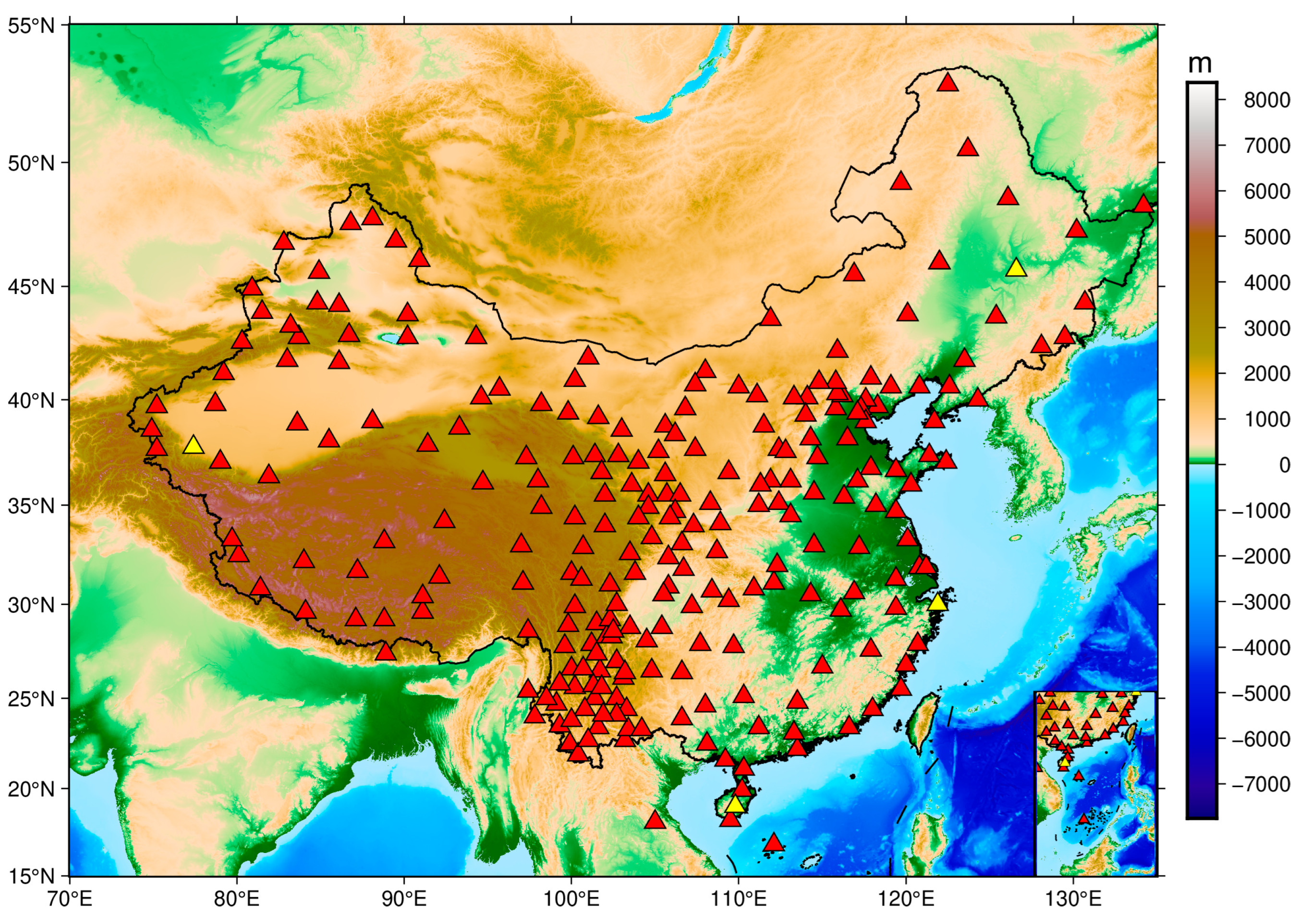
Figure 1. Geographic and topographic distribution of the 250 GNSS stations in China. The upward triangles denote GNSS stations, with yellow ones representing four randomly selected GNSS stations.
Remotesensing 17 03164 g001
Figure 2. Distribution of bias in different models validated using GNSS data for 2020 over China.
Remotesensing 17 03164 g002
Figure 3. Distribution of RMSE in different models validated using GNSS data for 2020 over China.
Remotesensing 17 03164 g003
Figure 4. The correlation coefficients between ZTD values estimated by different models and observed ZTD values are compared at 4 randomly selected representative stations on a 7-day forecast scale. The red solid line indicates the linear regression fit, while the black dashed line represents the ideal 1:1 reference line. GFS-7 (13 levels) represents the ZTD values calculated using the same pressure levels as Pangu-7, while GFS-7 (31 levels) represents the ZTD values calculated using all pressure levels of the GFS product. (a,d,g,j) Scatter density plot of Pangu-7 model predicted ZTD values and observed ZTD values at four stations. (b,e,h,k) Scatter density plot of GFS-7 (13 pressure levels) predicted ZTD values and observed ZTD values at four stations. (c,f,i,l) Scatter density plot of GFS-7 (31 pressure levels) predicted ZTD values and observed ZTD values at four stations.
Remotesensing 17 03164 g004
Figure 5. The correlation coefficients between ZTD values estimated by different models and observed ZTD values are compared at 4 randomly selected representative stations on a 14-day forecast scale. The red solid line indicates the linear regression fit, while the black dashed line represents the ideal 1:1 reference line. (a,d,g,j) Scatter density plot of Pangu-14 model predicted ZTD values and observed ZTD values at four stations. (b,e,h,k) Scatter density plot of GFS-14 (31 pressure levels) predicted ZTD values and observed ZTD values at four stations. (c,f,i,l) Scatter density plot of GPT3 model predicted ZTD values and observed ZTD values at four stations.
Remotesensing 17 03164 g005
Figure 6. (a) Results of bias of the different models at different latitude ranges. (b) Results of RMSE of the different models at different latitude ranges.
Remotesensing 17 03164 g006
Figure 7. (a) Results of bias of the different models at different altitude ranges. (b) Results of RMSE of the different models at different altitude ranges.
Remotesensing 17 03164 g007
Figure 8. Radar chart of bias and RMSE for different models at different months.
Remotesensing 17 03164 g008
Figure 9. (a,c) Hourly time series of the 7-day mean RMSE and ACC for different models; (b,d) corresponding magnified views of RMSE and ACC within the 0–40 h forecast range.
Remotesensing 17 03164 g009
Figure 10. (a,c) Hourly time series of the 14-day mean RMSE and ACC for different models; (b,d) corresponding magnified views of RMSE and ACC within the 199–275 h forecast range.
Remotesensing 17 03164 g010
Figure 11. Track of Typhoon Higos and the distribution of GXCORS.
Remotesensing 17 03164 g011
Figure 12. Time series of ZTD from the Pangu-Weather model and the GFS product at five GXCORS stations along the track of Typhoon Higos.
Remotesensing 17 03164 g012
Table 1. Spatiotemporal resolution and data types of each model used in this study.
DataTemporal
Resolution
Spatial
Resolution
Time
Latency
Data Type
GNSS5 s-Post-processingZenith total delays
Pangu-Weather1, 3, 6, 24 h0.25° × 0.25°ForecastedMeteorological parameters on pressure levels and surface
ERA51 h0.25° × 0.25°ReanalyzedMeteorological parameters on pressure levels and surface
GFS3 or 12 h0.25° × 0.25°ForecastedMeteorological parameters on pressure levels and surface
Table 2. Statistical results of different models validated at GNSS data for 2020.
ModelBias (cm)RMSE (cm)
MaxMinMeanMaxMinMean
Pangu-71.95−0.950.733.940.611.99
GFS-72.32−1.950.064.870.472.16
Pangu-142.26−0.940.815.740.682.94
GFS-142.78−2.290.165.940.702.98
GPT32.80−3.51−0.866.651.203.61
Table 3. Comparison of ZTD prediction performance between the Pangu-Weather model, the GFS product and the GPT3 empirical model at five GXCORS stations along the path of Typhoon Higos.
ModelPangu-ZTDGFS-ZTDGPT3-ZTD
RMSE (cm)Bias (cm)RMSE (cm)Bias (cm)RMSE (cm)Bias (cm)
J1044.28−3.445.14−4.138.30−6.94
J1002.62−1.382.96−2.056.33−5.04
J1032.97−2.334.22−3.167.39−6.17
JZ992.50−1.783.52−2.426.61−5.39
JZ951.710.432.23−0.464.52−3.22
Disclaimer/Publisher’s Note: The statements, opinions and data contained in all publications are solely those of the individual author(s) and contributor(s) and not of MDPI and/or the editor(s). MDPI and/or the editor(s) disclaim responsibility for any injury to people or property resulting from any ideas, methods, instructions or products referred to in the content.