Abstract
Deep learning has achieved remarkable success in hyperspectral image (HSI) classification, attributed to its powerful feature extraction capabilities. However, existing methods face several challenges: Convolutional Neural Networks (CNNs) are limited in modeling long-range spectral dependencies because of their limited receptive fields; Transformers are constrained by their quadratic computational complexity; and Mamba-based methods fail to fully exploit spatial–spectral interactions when handling high-dimensional HSI data. To address these limitations, we propose MRFP-Mamba, a novel Multi-Receptive-Field Parallel Mamba architecture that integrates hierarchical spatial feature extraction with efficient modeling of spatial–spectral dependencies. The proposed MRFP-Mamba introduces two key innovation modules: (1) A multi-receptive-field convolutional module employing parallel , , , and kernels to capture fine-to-coarse spatial features, thereby improving discriminability for multi-scale objects; and (2) a parameter-optimized Vision Mamba branch that models global spatial–spectral relationships through structured state space mechanisms. Experimental results demonstrate that the proposed MRFP-Mamba consistently surpasses existing CNN-, Transformer-, and state space model (SSM)-based approaches across four widely used hyperspectral image (HSI) benchmark datasets: PaviaU, Indian Pines, Houston 2013, and WHU-Hi-LongKou. Compared with MambaHSI, our MRFP-Mamba achieves improvements in Overall Accuracy (OA) by 0.69%, 0.30%, 0.40%, and 0.97%, respectively, thereby validating its superior classification capability and robustness.
1. Introduction
Hyperspectral images capture both rich spatial information and continuous spectral data across multiple bands, facilitating the identification of subtle feature differences for applications in precision agriculture [1], environmental monitoring [2], urban planning [3], and geological exploration [4,5,6]. However, the high data dimensionality, limited training samples, and need for efficient spatial–spectral integration pose challenges in fully leveraging this rich information.
HSI classification aims to divide pixels into categorical labels by jointly leveraging spatial context and spectral information. The traditional methods bifurcate into two paradigms: spectral-only classifiers (e.g., Support Vector Machines (SVMs) [7,8], Random Forest (RF) [9], and k-Nearest Neighbors (KNNs) [10,11,12,13] and shallow hybrid models (e.g., Principal Component Analysis (PCA) [14,15] and Linear Discriminant Analysis (LDA) [16,17]. While these methods achieve baseline performance, they suffer from three critical flaws: (1) neglect of spatial information, leading to misclassification of spectrally similar classes; (2) vulnerability to the “curse of dimensionality” due to redundant spectral bands; and (3) poor generalization under limited training samples.
Recently, deep learning techniques have achieved significant progress in hyperspectral image (HSI) classification. There are many Convolutional Neural Network (CNN)-based methods for HSI classification [18,19]. For example, Yang et al. [20] employed a fusion strategy combining 2D-CNN and 3D-CNN [21] to effectively extract deep features from limited HSI samples. Roy et al. [7] introduced HybridSN, which integrates 3D-CNN for local spatial–spectral feature extraction and further leverages 2D-CNN to model deep hierarchical features, thereby improving classification accuracy. These CNN-based methods advanced the field by extracting joint spatial–spectral features, yet their localized receptive fields hinder long-range dependency capture.
Transformer-based architectures addressed this via self-attention mechaisms to model the long-range dependencies. For example, He et al. [22] applied Transformer structures to HSI classification and proposed the SSF model, which integrates CNNs for local spatial feature extraction while utilizing Transformers for spectral sequence modeling. Graham et al. [23] incorporated convolutional operations before the Transformer module to extract local features before performing global modeling. Moreover, Mei et al. [24] introduced the GAHT architecture, which combines CNNs and Transformers to capture local dependencies between spectral channels and employs a hierarchical Transformer for feature representation. Xu et al. [25] proposed the Dual Selective Fusion Transformer Network (DSFormer), which adaptively selects and fuses spatial–spectral features from multiple receptive fields to enable joint modeling, thereby significantly improving classification accuracy across several benchmark datasets. Cheng et al. [26] developed CACFTNet, which integrates a covariance attention mechanism with cross-layer fusion strategies to enhance feature extraction capability, demonstrating outstanding performance especially in complex land-cover scenarios. Although Transformers excel at capturing long-range dependencies, their computational complexity increases quadratically with the input sequence length. This poses substantial challenges in terms of resource consumption when processing high-dimensional hyperspectral data. The resulting high computational cost limits their scalability in practical applications, making deployment particularly difficult in real-time processing scenarios or environments with constrained hardware resources.
Now, Mamba-based models emerge as efficient alternatives with linear scalability. Mamba integrates convolutional operations with state space modeling (SSM) modules, enabling efficient long-range dependency capture while maintaining significantly lower computational complexity compared to Transformers, making it particularly well-suited for long-sequence modeling tasks. For example, SpectralMamba [27] focuses on spectral dimension modeling, whereas 3DSS-Mamba incorporates both spatial and spectral information, further enhancing the capability of SSM-based approaches in processing hyperspectral data. However, the current Mamba models still face two major challenges in the field of hyperspectral image (HSI) classification.
- Spatial–spectral Decoupling in Mamba Variants: While these methods excel at modeling sequential spectral patterns (e.g., distinguishing subtle reflectance variations between vegetation species), they inadequately integrate spatial hierarchies—the multi-scale geometric and contextual relationships between pixels.
- Scale Sensitivity of Single-Receptive-Field Convolutions: Current HSI classification methods rely on fixed-size convolutional kernels or attention windows, which restrict their ability to capture multi-granular spatial features.
To address the challenges of spatial–spectral decoupling and scale sensitivity in existing Mamba-based hyperspectral image (HSI) classification methods, we propose MRFP-Mamba, a novel Multi-Receptive-Field Parallel Mamba architecture that integrates hierarchical spatial feature extraction with efficient modeling of spatial–spectral dependencies. This architecture combines the strengths of multi-scale convolutional operations and structured state space modeling to achieve adaptive spatial feature extraction and long-range spectral dependency capture, enhancing discriminative power for complex HSI classification tasks. Specifically, the proposed MRFP-Mamba comprises two core innovative modules: (1) a multi-receptive-field convolutional module (MRFCM) to capture fine-grained details (via smaller kernels) and coarse-grained contextual information (via larger kernels), effectively addressing scale sensitivity in single-receptive-field convolutions; (2) a parameter-optimized Vision Mamba branch to model global spatial–spectral dependencies. The contributions are listed as follows:
- We propose MRFP-Mamba, a hierarchical architecture that combines multi-receptive-field convolutional feature extraction with a parameter-optimized Vision Mamba, enabling adaptive capture of multi-scale spatial features and efficient modeling of global spectral dependencies.
- We introduce a multi-receptive-field convolutional module to extract hierarchical spatial features, addressing scale sensitivity issues in single-kernel convolutions. This module captures fine-grained details and coarse contextual information simultaneously, improving representation of multi-scale objects and spatial–spectral interactions.
- We design a parameter-optimized Vision Mamba branch that models long-range spectral dependencies across bands, enabling effective fusion of local spatial hierarchies and global spectral correlations.
- Extensive experiments on four HSI datasets demonstrate that MRFP-Mamba outperforms state-of-the-art HSI classification methods, achieving significant improvements in Overall Accuracy (OA).
The remainder of this paper is organized as follows. Section 2 reviews related work on hyperspectral image classification based on CNNs, Transformers, and Mamba models. Section 3 presents the proposed MRFP-Mamba model and its key components. Section 4 introduces the four benchmark HSI datasets, describes the experimental setup, and provides the results and analysis. Finally, Section 5 concludes the paper.
2. Related Works
HSI classification methods aim to integrate the rich spatial and spectral information to distinguish subtle land cover differences. This section reviews three key paradigms: Convolutional Neural Networks (CNNs), Transformers, and Mamba-based HSI classification models.
2.1. Convolution Neural Networks for Hyperspectral Image Classification
Convolutional Neural Networks (CNNs) have been widely applied in hyperspectral image (HSI) analysis due to their strong capability for local feature extraction [28,29,30,31]. Traditional 2D-CNN architectures, such as the design in [28,31,32], process spatial and spectral dimensions separately, achieving moderate classification accuracy but failing to model inter-band correlations effectively. To address this limitation, 3D-CNNs like [7,31], were introduced, using volumetric convolutions to jointly extract spatial–spectral features from 3D data cubes. For example, HybridSN [7], which combines 3D convolutions for local spatial–spectral feature extraction with 2D convolutions for hierarchical spatial refinement, improves performance on datasets like Indian Pines. However, these methods face two fundamental limitations. First, 2D-CNNs are constrained by limited receptive fields, leading to misclassifications in scenarios where distant spatial contexts are critical due to insufficient modeling of spatial texture differences. Second, 3D-CNNs suffer from excessive computational complexity, as their parameter counts grow cubically with input dimensions, making them impractical for large HSIs with hundreds of spectral bands.
RNNs have been applied to HSI classification for their ability to model spectral continuity in sequential data. Hang et al. [33] proposed a cascaded RNN architecture aimed at reducing redundancy between adjacent spectral bands and improving feature representation capability. Mei et al. [34] combined CNNs and RNNs, constructing a spatial–spectral fusion framework where CNNs extract spatial features while RNNs capture spectral dependencies. Additionally, an increasing number of deep learning architectures, such as Fully Convolutional Networks (FCNs), Generative Adversarial Networks (GANs), and Graph Convolutional Networks (GCNs), have been explored for HSI classification, each enhancing feature modeling capabilities to varying degrees.
Despite these advances, deep learning-based HSI classification still faces several challenges. For instance, RNNs struggle with capturing long-range dependencies, limiting their ability to model distant spectral relationships effectively. Meanwhile, CNNs are constrained by their limited receptive fields, making them less effective at extracting long-range spatial–spectral dependencies. These challenges restrict further improvement of existing methods in HSI classification. Therefore, it remains crucial to explore more efficient architectures that can optimize feature extraction strategies and achieve deeper fusion of spatial and spectral information.
2.2. Transformer Networks for Hyperspectral Image Classification
Transformers have emerged as a transformative approach in HSI classification [22,35,36,37,38], utilizing self-attention mechanisms to model global dependencies across spatial and spectral domains. Early works like SSF integrate CNNs for local feature extraction with transformers for spectral sequence modeling, demonstrating improved accuracy on small-scale datasets. More recently, advanced architectures such as SSFTT [39] and GAHT [24] have refined this paradigm: SSFTT decomposes HSI data into spectral and spatial tokens for independent modal refinement before fusion while GAHT employs grouped pixel embedding to constrain self-attention within local spectral contexts, reducing computational redundancy. These models integrate various innovative components that not only enhance the learning of local spectral features but also optimize the alignment between deep semantic features and sample distributions while improving the efficiency of skip connections. Leveraging these techniques, Transformer-based models have demonstrated superior performance in HSI classification compared to conventional Transformers, highlighting their significant application potential.
Although existing Transformer networks can effectively capture long-range dependencies, they often overlook local features. To address this issue, Wu et al. [40] proposed a novel Transformer network, Convolutional Vision Transformer (CvT), which integrates convolutional operations and self-attention mechanisms within its block structure. In this design, convolutional operations are responsible for extracting local features, while the self-attention mechanism captures global representations. However, these Transformer models only employ convolutional operations for local feature extraction and fail to fully exploit the complementary advantages of CNNs and Transformers.
To bridge this gap, Yang et al. [20] incorporated CNNs into Transformers and proposed a novel Transformer-based network, HSI Transformer (HiT). Zhou et al. [41] proposed the Dual-Branch Convolutional Transformer Network (DCTN), which employs a dual-branch structure to separately process spatial and spectral information. It integrates a spatial–spectral Fusion Projection Module (SFPM) and an Efficient Interactive Self-Attention (EISA) mechanism to enhance feature extraction and fusion, leading to improved classification performance across multiple datasets. Although transformers excel at encoding global contextual information, their scalability limitations in high-dimensional HSI spaces necessitate a shift toward more efficient architectures with linear computational complexity.
2.3. Mamba Networks for Hyperspectral Image Classification
As an emerging structured state space model (SSM), Mamba [42] has gained significant attention in natural language processing and computer vision due to its efficient long-range dependency modeling capabilities. Unlike Transformers, which rely on self-attention mechanisms for feature modeling, Mamba captures long-range dependencies with linear complexity through implicit state representations and selective filtering mechanisms, offering a novel approach for hyperspectral image (HSI) classification.
Recently, several studies have explored the application of the Mamba architecture in HSI tasks [43]. For instance, Yao et al. [27] proposed SpectralMamba, integrating PSS and GSSM modules to enhance sequential learning in the state domain and rectify spectral information, respectively. He et al. [44] proposed a 3D state space model (3D-SSM) to simultaneously model spatial and spectral information, enhancing feature representation while maintaining computational efficiency. However, this approach primarily relies on global information modeling and struggles to effectively capture local spatial features. Additionally, Vision Mamba, an extension of Mamba for computer vision [45], has demonstrated strong capabilities in modeling spatial information in 2D images. Nonetheless, when directly applied to HSI classification, it still faces challenges in adequately leveraging spectral information. Existing Mamba-based HSI classification methods remain in the exploratory stage and lack effective mechanisms for integrating spatial and spectral features in HSI data. Therefore, developing a method that combines Mamba with local spatial feature extraction modules for efficient HSI classification remains an important research direction.
To address this challenge, this study proposes an innovative approach that thoroughly analyzes the impact of channel dimensions on parameter complexity in Vision Mamba and integrates a multi-receptive field convolutional feature extraction module with a parallel Mamba architecture. This design significantly reduces parameter complexity while further enhancing local spatial feature extraction capabilities. Specifically, we introduce a multi-receptive field local feature extraction framework that captures multi-scale spatial information through different receptive field sizes, thereby facilitating the effective integration of spatial and spectral features in HSI data. This approach not only efficiently models the spatial–spectral relationships in hyperspectral images but also reduces the parameter count of Vision Mamba, improving its scalability for large-scale datasets.
3. Proposed Methodology
3.1. Preliminary
State space models (SSMs) are widely employed to characterize the dynamic behavior of a system. The fundamental concept involves mapping a one-dimensional input sequence to an output sequence via an intermediate latent state variable . In classical SSMs, the evolution of the system’s state is described by the following ordinary differential equations (ODEs):
where , , , and represent the state transition matrix, the input-to-state mapping matrix, the state-to-output mapping matrix, and the direct input-to-output mapping, respectively.
In order to incorporate SSMs into deep learning frameworks, a discretization of the continuous model is required. By introducing a time step , the system can be discretized as follows:
where the discretized system matrices are computed as
This discretization process is known as the Selective Scan Mechanism (S6). Unlike conventional Linear Time-Invariant (LTI) state-space models, S6 introduces a dynamic adjustment strategy that modifies system matrices based on both past and present input sequence information. This adaptability effectively overcomes the inherent constraints of LTI SSMs, which struggle to capture long-range dependencies in sequential data.
By allowing system matrices to be updated dynamically, the S6 mechanism enhances the flexibility of spatial and temporal modeling in visual sequence data. This capability is particularly advantageous for deep learning applications as it enables the effective extraction of complex, evolving patterns in image sequences.
3.2. Overview of MRFP-Mamba
Figure 1 illustrates the detailed architecture of the proposed MRFP-Mamba model, which consists of two main components. The first component is the multi-receptive field convolutional feature extraction module, which employs convolutional kernels of different sizes to capture local spatial information, thereby enhancing the hierarchical representation of spatial features. The second component is the parallel Vision Mamba structure, which leverages structured state space models (SSMs) to model long-range dependencies and improve spatial–spectral feature fusion.
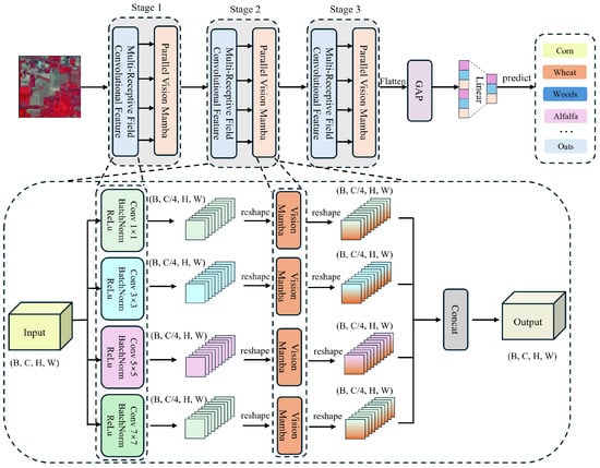
Figure 1.
The proposed MRFP-Mamba model architecture for HSI classification. The network consists of three structurally identical stages. Each stage comprises a multi-scale receptive field convolution feature extraction module, with convolution kernels of size , , , and , and a parallel Vision Mamba module. The multi-scale receptive field convolution module efficiently captures fine-grained and large-scale spatial features through the collaborative effect of different receptive fields. To reduce the number of parameters in the Vision Mamba module, the input channels are equally split into four branches for parallel processing, significantly improving computational efficiency and modeling capability. The complete algorithm flow is detailed in Algorithm 1.
After processing through three layers of multi-receptive field convolutional feature extraction and parallel Mamba operations, the features are further refined through global average pooling and a linear classification layer to obtain the final prediction results. The following sections provide a detailed explanation of the multi-receptive field convolutional feature extraction module and the parallel Vision Mamba structure.
3.3. Multi-Receptive Field Convolutional Feature Extraction
Hyperspectral images (HSIs) encapsulate rich spatial contextual details, yet single-scale convolutional layers often fail to comprehensively capture multi-granular local features critical for discriminative representation. To address this limitation, we introduce a multi-receptive-field convolutional feature extraction module, which leverages parallel convolutional branches with diverse kernel sizes to concurrently extract spatial features across multiple scales.
| Algorithm 1 MRFP-Mamba Implementation Process |
|
Specifically, the input features are processed through four parallel 2D convolutional layers with kernel sizes , , , and . Each branch independently generates feature maps that are subsequently normalized via Batch Normalization (BatchNorm) and activated by the ReLU function to enhance discriminative power. Mathematically, the operations are defined as follows.
Given the input feature , the MRFCFE module employs four different convolution operations:
where represents the convolution kernel of size , denotes the batch normalization operation, and is the activation function (e.g., ReLU). This parallel architecture enables the simultaneous extraction of fine-grained details (via smaller kernels) and coarse contextual information (via larger kernels), effectively resolving the scale sensitivity issue inherent in single-receptive-field designs and enhancing the model’s ability to represent multi-scale spatial structures in HSIs.
3.4. Parallel Mamba Structure for Long-Range Spatial–Spectral Dependency Modeling
3.4.1. Vision Mamba Parameter Impact Analysis
As a state-space model (SSM)-based architercture, Vision Mamba’s parameter size is influenced by several key factors, including the number of input channels, the dimensionality of the SSM state, the kernel size of the internal 1D convolution, the expansion ratio of projection layers, and the rank of the stride operation. Among these, the number of input channels plays the most crucial role in determining the model’s overall parameter count. To gain deeper insights into how these components contribute to model complexity, this study provides a comprehensive analysis from multiple perspectives.
In Vision Mamba (see Figure 2), represents the expanded projection channels, determined by the input channel size and the projection expansion factor (with a default value of 2). The equation for this relationship is
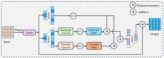
Figure 2.
Detailed architecture of Vision Mamba.The framework primarily consists of bidirectional (forward–backward) state space models, linear layers, and residual connections, achieving global contextual modeling with linear computational complexity.
This means increases multiplicatively with the increase in input channels, significantly influencing the model’s parameter count.
In addition, the input and output projection layers are directly related to and . The input projection layer () maps the input channels to , while the output projection layer () maps back to . The specific parameter calculation formulas are as follows:
The parameter count of these projection layers is directly proportional to the product of and , meaning that an increase in the number of input channels significantly raises the parameter count of these layers.
Then, the linear projection layers in the state-space model and are also related to and . maps to ( + ), while maps to . The parameter count formulas for these layers are as follows:
where is the rank of the step, given by , and denotes the size of the state dimension (usually fixed to 16). Therefore, an increase in leads to an increase in , thereby increasing the parameter count of these projection layers.
Lastly, in Vision Mamba, the convolutional layers usually perform convolution operations on the input using , where the size of the convolutional kernel is directly related to . An increase in leads to an increase in the parameter count of the convolutional layers. In the SSM module, is a parameter matrix with shape , so an increase in significantly increases the parameter count of this matrix.
From the above analysis, it is clear that has a big influence on the model’s parameter count. Specifically, more leads to more , which multiplies the parameter count across layers. Experimental results demonstrate that the parameter size of the Vision Mamba structure is significantly influenced by the number of input channels. When the input channel size is set to , the total number of parameters reaches 437,760. However, reducing the input channels to drastically decreases the parameter count to 32,640, representing a 92.54% reduction. In this study, we maintain the total number of channels while equally dividing them into four branches for input. This approach reduces the total parameter count to 130,560, achieving a 70.82% reduction compared to the non-branching case. These findings highlight the critical role of input channel configuration in controlling the parameter size of Vision Mamba and suggest that proper channel partitioning can effectively reduce model parameters while preserving computational capacity.
3.4.2. Parallel Vision Mamba Module
The multi-scale features generated by the MRFCFE module are not directly concatenated but are separately processed through independent Vision Mamba branches:
This design ensures that each Vision Mamba module processes features with a specific receptive field, preserving multi-scale spatial characteristics while leveraging Mamba’s state-space modeling capabilities to enhance long-range spectral dependencies. The Parallel Vision Mamba (PVM) architecture then integrates the processed features through channel-wise concatenation:
Here, represents the output of the Mamba processing for each receptive field branch. The concatenated feature tensor combines the local spatial information extracted by MRFCFE with the global spectral context modeled by Vision Mamba, constructing a powerful feature representation that captures both multi-scale spatial patterns and long-range dependencies in hyperspectral data.
For classification, the PVM features first undergo global average pooling (GAP):
The final model output (prediction) is given by a linear layer:
Here, F denotes the globally averaged pooled features obtained from the parallel Vision Mamba and MRFCFE feature extraction framework. This linear layer directly maps the features to the classification space, which can then be followed by softmax for probability computation or used for loss calculation.
4. Experiments
We selected four hyperspectral image (HSI) datasets, including Indian Pines, Pavia University, Houston 2013, and WHU-Hi-LongKou, to evaluate our proposed method. The experiments included classification result analysis, parameter analysis, and ablation studies.
4.1. Datasets
4.1.1. Indian Pines Dataset
The Indian Pines dataset was collected in 1992 using the Airborne Visible/Infrared Imaging Spectrometer (AVIRIS), manufactured by NASA Jet Propulsion Laboratory (JPL), Pasadena, CA, USA. over Northwestern Indiana, specifically covering an area with Indian pine trees. The spectrometer captures wavelengths ranging from 0.4 to 2.5 μm. After removing water absorption bands, the dataset retains 200 spectral bands with a spatial resolution of 20 m per pixel, covering a total area of pixels. It consists of 10,249 labeled pixels spanning 16 land cover classes, including categories such as Alfalfa and Corn-notill. The specific data partitioning used in our experiments is detailed in Table 1.

Table 1.
Number of training and testing samples for the Indian Pines dataset.
4.1.2. Pavia University Dataset
The Pavia University (PU) dataset was collected in 2001 using the ROSIS sensor, capturing 115 spectral bands within the wavelength range of 380 nm to 860 nm. After removing noisy bands, 103 spectral bands were retained for analysis. The dataset consists of an image with a spatial resolution of pixels and includes 42,776 labeled samples spanning nine land cover categories. For experimentation, 1% of the labeled data is allocated for training, while the remaining 99% is reserved for testing. This partitioning strategy ensures a robust model evaluation and a thorough assessment of classification performance, as detailed in Table 2.
Table 2.
Number of training and testing samples for the Pavia University dataset.
4.1.3. Houston 2013 Dataset
The Houston 2013 dataset is a publicly accessible hyperspectral dataset acquired using an Airborne Laser Mapping (ALM) system equipped with a 2.5 μm wavelength laser. The data were collected in the summer of 2013 over Houston, Texas, USA and were initially introduced as part of the 2013 IEEE GRSS Data Fusion Competition. The dataset consists of an image with a spatial resolution of pixels, captured from an aircraft flying at an altitude of 500 m between 12:30 p.m. and 4:30 p.m. on 18 June 2013. It includes 15 distinct land cover categories with a total of 15,029 labeled samples. For experimental purposes, 10% of the labeled data was allocated for training, while the remaining 90% was designated for testing, as detailed in Table 3.
Table 3.
Number of training and testing samples for the Houston 2013 dataset.
4.1.4. WHU-Hi-LongKou Dataset
The WHL dataset was captured using a Headwall Nano-Hyperspec imaging sensor with an 8 mm focal length, mounted on a DJI Matrice 600 Pro UAV (manufactured by DJI Technology Co., Ltd., Shenzhen, China). The UAV operated at an altitude of 500 m, producing hyperspectral images with a spatial resolution of 0.463 m per pixel. The dataset consists of a pixel image spanning 270 spectral bands within the 400–1000 nm wavelength range. It includes a total of 203,523 labeled samples categorized into 9 distinct land cover types. For evaluation, we allocated 0.5% of the labeled data for training and reserved the remaining 99.5% for testing, as summarized in Table 4.
Table 4.
Number of training and testing samples for the WHU-Hi-LongKou dataset.
4.2. Experimental Setup
4.2.1. Implementation Details
To facilitate a fair and efficient performance assessment, the proposed MRFP-Mamba architecture was implemented within the PyTorch 2.1.1 framework and deployed on an NVIDIA GeForce RTX 4090 GPU (manufactured by NVIDIA Corporation, Santa Clara, CA, USA). For training, 100 non-overlapping () pixel patches were randomly extracted from each dataset to construct the input feature space, ensuring representative sampling of spatial–spectral contexts. The training procedure spanned 100 epochs, leveraging the Adam optimizer with an initial learning rate of () and a consistent mini-batch size of 100 across all experimental setups. Model performance was quantified using three standard evaluation metrics: Overall Accuracy (OA) for global classification correctness, Average Accuracy (AA) to assess class-wise consistency, and the Kappa coefficient () to measure agreement beyond random chance. This configuration balances computational efficiency with rigorous validation, ensuring reliable comparison against state-of-the-art baselines.
4.2.2. Comparison with State-of-the-Art Backbone Methods
To validate the proposed method, we benchmark against a diverse set of state-of-the-art classification networks spanning CNN, Transformer, and Mamba architectures: 2D-CNN [46], 3D-CNN [47], ViT [48], Deep-ViT [49], HiT [20], SSFTT [39], GAHT [24], DCTN [41], MambaHSI [50] and 3DSS-Mamba [44].
Conventional CNN-based approaches serve as foundational baselines: 2D-CNNs employ standard convolutional layers with batch normalization and ReLU activation to extract spatial features while 3D-CNNs extend this to volumetric operations, jointly modeling spectral and spatial dimensions through 3D kernels. In contrast, ViT introduces a paradigm shift by leveraging linear projection and transformer encoders to model global contextual dependencies across spectral bands, though at the cost of quadratic complexity.
Transformer variants refine this framework with specialized designs: HiT integrates a Spectral-Adaptive 3D Convolution Projection (SACP) module and Convolutional Permutator to enhance spatial–spectral interactions, while SSFTT decomposes HSI data into spectral and spatial tokens for independent refinement, improving local structure learning and semantic alignment. GAHT mitigates global attention’s computational and representational challenges through a Grouped Pixel Embedding strategy, constraining Multi-Head Self-Attention (MHSA) within localized spectral contexts to reduce feature dispersion.
Mamba-based baselines, such as 3DSS-Mamba, adopt structured state space models (SSMs) for efficient long-range modeling, combining 3D state representations with linear-complexity operations across spectral and spatial axes.
The proposed MRFP-Mamba distinguishes itself by introducing a parallel architecture that fuses a multi-receptive-field convolutional module with a parameter-optimized Vision Mamba branch. This design jointly enhances local spatial feature extraction and global spectral dependency modeling, addressing key limitations of both CNN and Transformer paradigms.
4.3. Results and Analysis
We conduct experiments on four widely used hyperspectral image (HSI) datasets and evaluate the results using three metrics. The outcomes are summarized in Table 5, Table 6, Table 7 and Table 8, with the best results highlighted in bold.
Table 5.
Classification results of the Indian Pines dataset with 10% training samples. All bolded values indicate the best results. This applies to all the following tables.
Table 6.
Classification results of the PaviaU dataset with 1% training samples.
Table 7.
Classification results of the Houston 2013 dataset with 10% training samples.
Table 8.
Classification results of the WHU-Hi-LongKou dataset with 0.5% training samples.
From Table 5, Table 6, Table 7 and Table 8, it can be seen that the proposed MRFP-Mamba achieves notable improvements in classification performance across four widely used hyperspectral image (HSI) datasets, thereby validating the effectiveness of the proposed multi-receptive field parallel Mamba architecture in HSI classification tasks. Compared with conventional 2D convolutional neural networks (2D-CNNs), MRFP-Mamba integrates a multi-receptive field convolutional feature extraction module which enables the simultaneous capture of fine-grained local features and large-scale contextual information. This design effectively addresses the limitations of traditional convolutional models, which struggle to model long-range dependencies due to their restricted receptive fields. On the four benchmark datasets, MRFP-Mamba outperforms 2D-CNNs in Overall Accuracy (OA) by 0.18%, 9.05%, 3.79%, and 0.68%, respectively.
Building on this analysis, we develop a parallel Vision Mamba module through a comprehensive examination of the Vision Mamba architecture’s parameter composition. This design drastically reduces the parameter count while concurrently enhancing the model’s capability to model long-range dependencies in both spatial and spectral domains. Experimental comparisons with 3DSS-Mamba demonstrate that MRFP-Mamba outperforms the baseline across all datasets, achieving improvements in Overall Accuracy (OA) of 0.22%, 0.52%, 0.16%, and 0.42%, respectively.
While 3DSS-Mamba employs 3D convolutions to extract joint spatial–spectral features, its spatial modeling capacity is constrained by single-scale convolutional kernels and the absence of an effective multi-scale fusion mechanism. This limitation hinders its ability to capture hierarchical spatial details, leading to inferior classification performance compared to MRFP-Mamba’s parallel architecture—where multi-receptive-field convolutions and structured state space modeling work synergistically to integrate multi-scale spatial contexts with global spectral dependencies.
In addition, we compared MRFP-Mamba with several Transformer-based state-of-the-art models, including ViT, DeepViT, HiT, SSFTT, and GAHT. The experimental results show that MRFP-Mamba consistently outperforms these methods across various evaluation metrics, further highlighting its competitiveness in HSI classification tasks. In the visualized classification maps shown in Figure 3, Figure 4, Figure 5 and Figure 6, MRFP-Mamba produces results with clearer boundaries, finer detail restoration, and stronger spatial consistency compared to the other models. These improvements can be attributed to the synergy between its multi-receptive field convolution module, which captures multi-scale spatial features, and the Vision Mamba, which excels at modeling contextual dependencies.
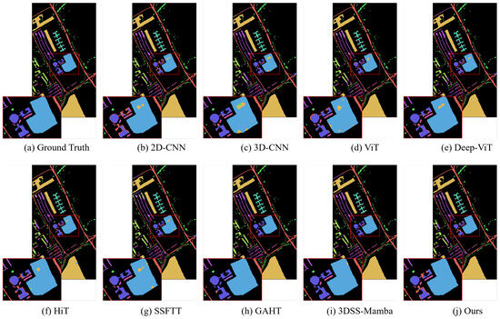
Figure 3.
Classification maps obtained using different methrods on the PaviaU dataset (with 1% training samples).
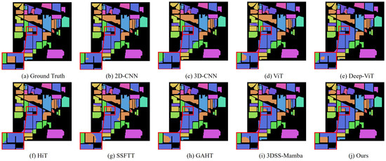
Figure 4.
Classification maps obtained using different methods on the Indian Pines dataset (with 10% training samples).
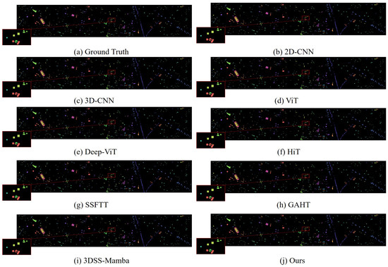
Figure 5.
Classification maps obtained using different methods on the Houston 2013 dataset (with 10% training samples).
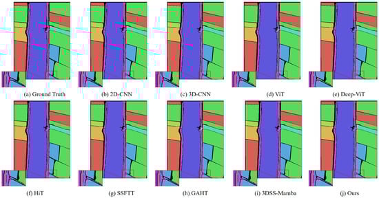
Figure 6.
Classification maps obtained using different methods on the WHU-Hi-LongKou dataset (with 0.5% training samples).
To further evaluate the model’s discriminative capability, we conducted a t-SNE visualization on the PaviaU dataset (as illustrated in Figure 7), comparing MRFP-Mamba with 2D-CNN, ViT, DeepViT, HiT, SSFTT, GAHT, DCTN, MambaHSI, and 3DSS-Mamba. The results show that MRFP-Mamba produces more compact and better separated class clusters in the feature space, significantly reducing inter-class confusion while enhancing intra-class cohesion. In contrast, 2D-CNN and 3DSS-Mamba display more dispersed and overlapping class distributions, indicating suboptimal performance in extracting either local or global features. Benefiting from the collaborative design of multi-receptive field convolutions and the parallel Vision Mamba, MRFP-Mamba achieves effective multi-scale spatial modeling and efficient long-range dependency capture, demonstrating superior accuracy and visual representation. Collectively, these findings underscore that developing a model capable of effectively integrating local and global features through a compact and efficient architecture is key to advancing the state of the art in hyperspectral image classification.
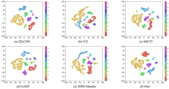
Figure 7.
Visualization of t-SNE data analysis on the PaviaU dataset.
Table 9 presents the classification performance of various methods on the Indian Pines and Houston 2013 datasets using only 5% of the training samples. On the Indian Pines dataset, the proposed method achieves the best results across all three metrics: Overall Accuracy (OA) at 92.18%, Average Accuracy (AA) at 77.61%, and Kappa coefficient at 91.07%, significantly outperforming other compared methods. For instance, compared to 3DSS-Mamba (which attains an OA of 89.23%), our method improves overall accuracy by nearly three percentage points, while also demonstrating notable advantages in AA and Kappa scores. Similarly, on the Houston 2013 dataset, the proposed method exhibits superior performance, achieving an OA of 96.55%, AA of 96.20%, and Kappa of 95.93%, surpassing all baseline methods. Notably, compared to DCTN, it attains an approximate one percentage point increase in OA, highlighting its strong classification capability and generalization performance. In summary, the proposed method demonstrates robust competitiveness in hyperspectral image classification across two distinct scenarios, confirming its effectiveness and robustness under low-sample training conditions.
Table 9.
Classification results of the Indian Pines and Houston 2013 datasets with 5% training samples.
We evaluated the model complexity of various methods on the Indian Pines dataset by measuring floating-point operations (FLOPs), number of parameters (Param), training time, and testing time, as summarized in Table 10. Notably, our proposed MRFP-Mamba method achieves strong performance across these metrics. From the perspective of computational complexity, traditional 2D-CNN models exhibit relatively low FLOPs and parameter counts, measuring 0.06 G and 1.67 MB respectively, accompanied by short training and testing times. In contrast, Transformer-based architectures such as the ViT model significantly increase computational demands, with FLOPs reaching 0.34 G and parameters totaling 6.54 MB, resulting in notably longer training and inference durations. Methods like GAHT and SSFTT demonstrate computational complexity that lies between conventional CNNs and ViT, reflecting moderate improvements in efficiency. Although the DCTN model achieves strong classification accuracy, it incurs the highest computational cost, with FLOPs of 2.95 G, 53.94 MB parameters, training time exceeding 441 s, and testing time of 7.93 s, indicating substantial resource consumption. Our proposed approach maintains moderate FLOPs and parameter levels (0.73 G FLOPs, 1.64 MB parameters), with training and testing times of 80.36 s and 3.86 s, respectively, substantially lower than DCTN but higher than traditional 2D-CNN- and certain Transformer-based methods. In terms of classification performance, our method attains the highest Overall Accuracy (94.46%), Average Accuracy (89.88%), and Kappa coefficient (93.67%), demonstrating superior comprehensive effectiveness. Furthermore, MambaHSI and 3DSS-Mamba exhibit extremely low FLOPs and parameter counts (both at 0.01 G FLOPs and approximately 0.42 MB parameters), yet their training times are relatively long, around 360 s. Compared to these, our method achieves a favorable balance between high classification accuracy and computational efficiency, highlighting its practical applicability and efficiency advantages in hyperspectral image classification tasks.
Table 10.
Comparison of computational complexity.
4.4. Ablation Studies
4.4.1. Ablation Study of the Input Size
As shown in Table 11, we investigate the impact of different input patch sizes on classification performance across three hyperspectral datasets. The input sizes range from to . The results demonstrate that classification accuracy varies with the change in input size. In most cases, smaller input patches tend to achieve higher Overall Accuracy (OA) and Kappa coefficient (). This may be attributed to the fact that smaller patches can better focus on local spatial details, thus extracting more representative fine-grained features for land cover discrimination. In contrast, larger input regions might introduce redundant or even noisy information, which could weaken feature discriminability and negatively impact classification. These observations further validate the robustness and adaptability of the proposed MRFP-Mamba under different input configurations.
Table 11.
Ablation study of the input size.
4.4.2. Ablation Study of Different Modules
As shown in Table 12, we conducted ablation experiments on the multi-receptive-field convolutional module. In the MRFP-Mamba model, there are three such modules composed of multi-receptive-field convolution and parallel Vision Mamba, with output channels of 256, 128, and 64, respectively. Accordingly, we designed ablation settings with pairwise combinations of convolution kernels of Sizes 1, 3, 5, and 7. The experimental results indicate that the combination of larger kernels (5 and 7) yields relatively poor performance (OA = ), which may be attributed to the fact that large kernels tend to introduce redundant information during feature extraction, thereby reducing the discriminability of local details. In contrast, the combination of all four kernel sizes (1, 3, 5, and 7) achieves the best result (), demonstrating that the full fusion of multi-scale information effectively captures spatial features at different granularities. These results further validate the importance of the proposed multi-receptive-field convolutional module in enhancing the representational capacity of the model.
Table 12.
Ablation study of the Different Modules on WHU-Hi-LongKou.
4.4.3. Ablation Study of the Numbers of the Training Samples
We conducted a systematic series of experiments on four representative hyperspectral image (HSI) datasets, examining the impact of varying training sample sizes. As illustrated in Figure 8, a clear upward trend in Overall Accuracy (OA) is observed as the number of training samples increases. This trend indicates that larger training sets significantly enhance the model’s discriminative capacity, particularly in distinguishing between different classes and reducing random misclassifications. These findings highlight the positive influence of expanded training data on the classification accuracy and robustness of the proposed method and further underscore the critical role of data scale in optimizing the performance of deep learning models.
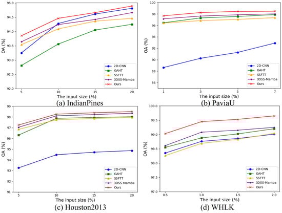
Figure 8.
OA of different models with different percentages training samples on four datasets.
4.5. Discussion
Through extensive experiments, we identified the strengths of MRFP-Mamba in its efficient spatial–spectral feature extraction and long-range dependency modeling. By leveraging the multi-receptive field convolutional feature extraction module, MRFP-Mamba is able to simultaneously capture fine-grained local features and broader contextual information, which enables it to perform excellently when handling the complexities of hyperspectral image (HSI) data. The parallel Vision Mamba architecture further enhances the model’s ability to capture long-range dependencies while maintaining linear complexity, thus improving its performance in HSI classification.
Moreover, the integration of these components allows MRFP-Mamba to effectively combine spatial and spectral information. The multi-receptive field convolution captures detailed spatial features, while the Vision Mamba structure efficiently models the relationships between these features, leading to better spatial–spectral fusion and improved classification accuracy. Extensive experimental results validate its effectiveness and highlight its potential for practical applications in HSI analysis.
5. Conclusions and Fulture Work
In this paper, we propose a novel Multi-Receptive-Field Parallel Mamba (MRFP-Mamba) framework for hyperspectral image (HSI) classification. This method integrates a multi-receptive-field convolutional feature extractor with a parallel Vision Mamba module, achieving a seamless fusion of local feature extraction and long-range spectral dependency modeling. Specifically, the multi-receptive-field convolutional structure is employed to capture spatial features at different scales, while Vision Mamba efficiently models spectral dependencies, thereby enhancing feature representation capability. Extensive experiments on multiple benchmark HSI datasets demonstrate that MRFP-Mamba outperforms existing CNN-, Transformer-, and SSM-based methods in classification accuracy. In addition to enhancing classification performance, our method also demonstrates superior computational efficiency. Compared to 3DSS-Mamba, it reduces training time by 77.46% and testing time by 49.74%, making it more suitable for large-scale hyperspectral applications. Furthermore, the introduction of the Mamba architecture provides a new paradigm for hyperspectral classification, addressing the computational complexity issues of traditional self-attention mechanisms and enhancing model scalability.
In future work, we plan to further explore adaptive receptive field learning to enhance spatial feature extraction and investigate more efficient spectral modeling methods to reduce computational costs while maintaining high classification accuracy. Moreover, extending MRFP-Mamba to self-supervised and semi-supervised learning holds great potential for improving its applicability in real-world remote sensing tasks.
Author Contributions
Conceptualization, X.Y.; methodology, L.L.; validation, L.L., S.X. and S.L.; formal analysis, X.Y., L.L. and H.T.; data curation, L.L. and X.Y.; writing—original draft, X.Y. and L.L.; funding acquisition, W.Y. and X.H.; writing—review and editing, X.Y., S.X., S.L. and L.L.; visualization, L.L.; supervision, W.Y. and X.H. All authors have read and agreed to the published version of the manuscript.
Funding
This work was supported in part by National Natural Science Foundation of China (NSFC) Fund under Grant 62301174 and Guangzhou basic and applied basic research topics under Grant 2024A04J2081 and Grant 2025A04J3375. This work also was supported in part by the National Natural Science Foundation of China under Grant No. 62462031, in part by the Natural Science Foundation of Jiangxi Province under Grant 20242BAB26023.
Data Availability Statement
The codes and parameters of our model are publicly available at https://github.com/Li-gzhu/MRFP-Mamba (accessed on 20 April 2025).
Conflicts of Interest
The authors declare no conflicts of interest.
References
- Gevaert, C.M.; Suomalainen, J.; Tang, J.; Kooistra, L. Generation of Spectral—Temporal Response Surfaces by Combining Multispectral Satellite and Hyperspectral UAV Imagery for Precision Agriculture Applications. IEEE J. Sel. Top. Appl. Earth Obs. Remote Sens. 2015, 8, 3140–3146. [Google Scholar] [CrossRef]
- Hestir, E.L.; Brando, V.E.; Bresciani, M.; Giardino, C.; Matta, E.; Villa, P.; Dekker, A.G. Measuring freshwater aquatic ecosystems: The need for a hyperspectral global mapping satellite mission. Remote Sens. Environ. 2015, 167, 181–195. [Google Scholar] [CrossRef]
- Chen, F.; Wang, K.; Voorde, T.V.D.; Tang, T.F. Mapping urban land cover from high spatial resolution hyperspectral data: An approach based on simultaneously unmixing similar pixels with jointly sparse spectral mixture analysis. Remote Sens. Environ. 2017, 196, 324–342. [Google Scholar] [CrossRef]
- Sun, L.; Wu, F.; Zhan, T.; Liu, W.; Wang, J.; Jeon, B. Weighted Nonlocal Low-Rank Tensor Decomposition Method for Sparse Unmixing of Hyperspectral Images. IEEE J. Sel. Top. Appl. Earth Obs. Remote Sens. 2020, 13, 1174–1188. [Google Scholar] [CrossRef]
- Wang, J.; Zhang, L.; Tong, Q.; Sun, X. The Spectral Crust project—Research on new mineral exploration technology. In Proceedings of the 2012 4th Workshop on Hyperspectral Image and Signal Processing: Evolution in Remote Sensing (WHISPERS), Shanghai, China, 4–7 June 2012; IEEE: Piscataway, NJ, USA, 2012; pp. 1–4. [Google Scholar]
- Zhang, Y.; Yan, S.; Jiang, X.; Zhang, L.; Cai, Z.; Li, J. Dual Graph Learning Affinity Propagation for Multimodal Remote Sensing Image Clustering. IEEE Trans. Geosci. Remote Sens. 2024, 62, 5521713. [Google Scholar] [CrossRef]
- Roy, S.K.; Krishna, G.; Dubey, S.R.; Chaudhuri, B.B. HybridSN: Exploring 3-D–2-D CNN Feature Hierarchy for Hyperspectral Image Classification. IEEE Geosci. Remote Sens. Lett. 2020, 17, 277–281. [Google Scholar] [CrossRef]
- Pasolli, E.; Melgani, F.; Tuia, D.; Pacifici, F.; Emery, W.J. SVM active learning approach for image classification using spatial information. IEEE Trans. Geosci. Remote Sens. 2013, 52, 2217–2233. [Google Scholar] [CrossRef]
- Ham, J.; Chen, Y.; Crawford, M.M.; Ghosh, J. Investigation of the random forest framework for classification of hyperspectral data. IEEE Trans. Geosci. Remote Sens. 2005, 43, 492–501. [Google Scholar] [CrossRef]
- Ma, L.; Crawford, M.M.; Tian, J. Local Manifold Learning-Based k -Nearest-Neighbor for Hyperspectral Image Classification. IEEE Trans. Geosci. Remote Sens. 2010, 48, 4099–4109. [Google Scholar] [CrossRef]
- Song, W.; Li, S.; Kang, X.; Huang, K. Hyperspectral image classification based on KNN sparse representation. In Proceedings of the 2016 IEEE International Geoscience and Remote Sensing Symposium (IGARSS), Beijing, China, 10–15 July 2016; IEEE: Piscataway, NJ, USA, 2016; pp. 2411–2414. [Google Scholar]
- Zhang, Y.; Wang, X.; Jiang, X.; Zhang, L.; Du, B. Elastic Graph Fusion Subspace Clustering for Large Hyperspectral Image. IEEE Trans. Circuits Syst. Video Technol. 2025. early access. [Google Scholar]
- Zhang, Y.; Jiang, G.; Cai, Z.; Zhou, Y. Bipartite Graph-based Projected Clustering with Local Region Guidance for Hyperspectral Imagery. IEEE Trans. Multimed. 2024, 26, 9551–9563. [Google Scholar] [CrossRef]
- Sheykhmousa, M.; MahdianPari, M.; Ghanbari, H.; Mohammadimanesh, F.; Ghamisi, P.; Homayouni, S. Support Vector Machine Versus Random Forest for Remote Sensing Image Classification: A Meta-Analysis and Systematic Review. IEEE J. Sel. Top. Appl. Earth Obs. Remote Sens. 2020, 13, 6308–6325. [Google Scholar] [CrossRef]
- Villa, A.; Benediktsson, J.A.; Chanussot, J.; Jutten, C. Hyperspectral Image Classification with Independent Component Discriminant Analysis. IEEE Trans. Geosci. Remote Sens. 2011, 49, 4865–4876. [Google Scholar] [CrossRef]
- Liao, W.; Pizurica, A.; Scheunders, P.; Philips, W.; Pi, Y. Semisupervised Local Discriminant Analysis for Feature Extraction in Hyperspectral Images. IEEE Trans. Geosci. Remote Sens. 2013, 51, 184–198. [Google Scholar] [CrossRef]
- Wang, Q.; Meng, Z.; Li, X. Locality Adaptive Discriminant Analysis for Spectral-Spatial Classification of Hyperspectral Images. IEEE Geosci. Remote Sens. Lett. 2017, 14, 2077–2081. [Google Scholar] [CrossRef]
- Dai, J.; Qi, H.; Xiong, Y.; Li, Y.; Zhang, G.; Hu, H.; Wei, Y. Deformable Convolutional Networks. In Proceedings of the 2017 IEEE International Conference on Computer Vision (ICCV), Venice, Italy, 22–29 October 2017; IEEE Computer Society: Piscataway, NJ, USA, 2017; pp. 764–773. [Google Scholar]
- Zhao, C.; Zhu, W.; Feng, S. Superpixel Guided Deformable Convolution Network for Hyperspectral Image Classification. IEEE Trans. Image Process. 2022, 31, 3838–3851. [Google Scholar] [CrossRef] [PubMed]
- Yang, X.; Cao, W.; Lu, Y.; Zhou, Y. Hyperspectral Image Transformer Classification Networks. IEEE Trans. Geosci. Remote Sens. 2022, 60, 5528715. [Google Scholar] [CrossRef]
- Ahmad, M.; Khan, A.M.; Mazzara, M.; Distefano, S.; Ali, M.; Sarfraz, M.S. A Fast and Compact 3-D CNN for Hyperspectral Image Classification. IEEE Geosci. Remote Sens. Lett. 2022, 19, 5502205. [Google Scholar] [CrossRef]
- He, X.; Chen, Y.; Lin, Z. Spatial-Spectral Transformer for Hyperspectral Image Classification. Remote Sens. 2021, 13, 498. [Google Scholar] [CrossRef]
- Graham, B.; El-Nouby, A.; Touvron, H.; Stock, P.; Joulin, A.; Jégou, H.; Douze, M. Levit: A vision transformer in convnet’s clothing for faster inference. In Proceedings of the IEEE/CVF International Conference on Computer Vision, Montreal, BC, Canada, 11–17 October 2021; pp. 12259–12269. [Google Scholar]
- Mei, S.; Song, C.; Ma, M.; Xu, F. Hyperspectral image classification using group-aware hierarchical transformer. IEEE Trans. Geosci. Remote Sens. 2022, 60, 5539014. [Google Scholar] [CrossRef]
- Xu, Y.; Wang, D.; Zhang, L.; Zhang, L. Dual selective fusion transformer network for hyperspectral image classification. Neural Networks 2025, 187, 107311. [Google Scholar] [CrossRef]
- Cheng, S.; Chan, R.; Du, A. CACFTNet: A Hybrid Cov-Attention and Cross-Layer Fusion Transformer Network for Hyperspectral Image Classification. IEEE Trans. Geosci. Remote Sens. 2024, 62, 1–17. [Google Scholar] [CrossRef]
- Yao, J.; Hong, D.; Li, C.; Chanussot, J. SpectralMamba: Efficient Mamba for Hyperspectral Image Classification. arXiv 2024, arXiv:2404.08489. [Google Scholar]
- Lee, H.; Kwon, H. Going Deeper with Contextual CNN for Hyperspectral Image Classification. IEEE Trans. Image Process. 2017, 26, 4843–4855. [Google Scholar] [CrossRef] [PubMed]
- Cao, X.; Zhou, F.; Xu, L.; Meng, D.; Xu, Z.; Paisley, J.W. Hyperspectral Image Classification with Markov Random Fields and a Convolutional Neural Network. IEEE Trans. Image Process. 2018, 27, 2354–2367. [Google Scholar] [CrossRef]
- Wang, Z.; Chen, B.; Lu, R.; Zhang, H.; Liu, H.; Varshney, P.K. FusionNet: An Unsupervised Convolutional Variational Network for Hyperspectral and Multispectral Image Fusion. IEEE Trans. Image Process. 2020, 29, 7565–7577. [Google Scholar] [CrossRef]
- Li, Y.; Zhang, H.; Shen, Q. Spectral-Spatial Classification of Hyperspectral Imagery with 3D Convolutional Neural Network. Remote Sens. 2017, 9, 67. [Google Scholar] [CrossRef]
- Zhang, Y.; Yan, S.; Zhang, L.; Du, B. Fast Projected Fuzzy Clustering with Anchor Guidance for Multimodal Remote Sensing Imagery. IEEE Trans. Image Process. 2024, 33, 4640–4653. [Google Scholar] [CrossRef]
- Hang, R.; Liu, Q.; Hong, D.; Ghamisi, P. Cascaded recurrent neural networks for hyperspectral image classification. IEEE Trans. Geosci. Remote Sens. 2019, 57, 5384–5394. [Google Scholar] [CrossRef]
- Mei, X.; Pan, E.; Ma, Y.; Dai, X.; Huang, J.; Fan, F.; Du, Q.; Zheng, H.; Ma, J. Spectral-spatial attention networks for hyperspectral image classification. Remote Sens. 2019, 11, 963. [Google Scholar] [CrossRef]
- Yang, X.; Cao, W.; Tang, D.; Zhou, Y.; Lu, Y. ACTN: Adaptive Coupling Transformer Network for Hyperspectral Image Classification. IEEE Trans. Geosci. Remote Sens. 2025, 63, 5503115. [Google Scholar] [CrossRef]
- Xu, Y.; Du, B.; Zhang, L. Self-Attention Context Network: Addressing the Threat of Adversarial Attacks for Hyperspectral Image Classification. IEEE Trans. Image Process. 2021, 30, 8671–8685. [Google Scholar] [CrossRef]
- Hong, D.; Han, Z.; Yao, J.; Gao, L.; Zhang, B.; Plaza, A.; Chanussot, J. SpectralFormer: Rethinking Hyperspectral Image Classification With Transformers. IEEE Trans. Geosci. Remote Sens. 2022, 60, 5518615. [Google Scholar] [CrossRef]
- Ouyang, E.; Li, B.; Hu, W.; Zhang, G.; Zhao, L.; Wu, J. When Multigranularity Meets Spatial-Spectral Attention: A Hybrid Transformer for Hyperspectral Image Classification. IEEE Trans. Geosci. Remote Sens. 2023, 61, 1–18. [Google Scholar] [CrossRef]
- Xu, Y.; Xie, Y.; Li, B.; Xie, C.; Zhang, Y.; Wang, A.; Zhu, L. Spatial-Spectral 1DSwin Transformer with Groupwise Feature Tokenization for Hyperspectral Image Classification. IEEE Trans. Geosci. Remote Sens. 2023, 61, 5516616. [Google Scholar] [CrossRef]
- Wu, H.; Xiao, B.; Codella, N.; Liu, M.; Dai, X.; Yuan, L.; Zhang, L. CvT: Introducing Convolutions to Vision Transformers. In Proceedings of the IEEE/CVF International Conference on Computer Vision (ICCV), Montreal, QC, Canada, 10–17 October 2021; IEEE: Piscataway, NJ, USA, 2021; pp. 22–31. [Google Scholar]
- Zhou, Y.; Huang, X.; Yang, X.; Peng, J.; Ban, Y. DCTN: Dual-Branch Convolutional Transformer Network with Efficient Interactive Self-Attention for Hyperspectral Image Classification. IEEE Trans. Geosci. Remote Sens. 2024, 62, 5508616. [Google Scholar] [CrossRef]
- Gu, A.; Dao, T. Mamba: Linear-Time Sequence Modeling with Selective State Spaces. arXiv 2023, arXiv:2312.00752. [Google Scholar]
- Lu, S.; Zhang, M.; Huo, Y.; Wang, C.; Wang, J.; Gao, C. SSUM: Spatial—Spectral Unified Mamba for Hyperspectral Image Classification. Remote Sens. 2024, 16, 4653. [Google Scholar] [CrossRef]
- He, Y.; Tu, B.; Liu, B.; Li, J.; Plaza, A. 3DSS-Mamba: 3D-Spectral-Spatial Mamba for Hyperspectral Image Classification. IEEE Trans. Geosci. Remote Sens. 2024, 62, 5534216. [Google Scholar] [CrossRef]
- Wu, R.; Liu, Y.; Liang, P.; Chang, Q. UltraLight VM-UNet: Parallel Vision Mamba Significantly Reduces Parameters for Skin Lesion Segmentation. arXiv 2024, arXiv:2403.20035. [Google Scholar]
- Liu, B.; Yu, X.; Zhang, P.; Tan, X.; Yu, A.; Xue, Z. A semi-supervised convolutional neural network for hyperspectral image classification. Remote Sens. Lett. 2017, 8, 839–848. [Google Scholar] [CrossRef]
- Sharma, V.; Diba, A.; Tuytelaars, T.; Van Gool, L. Hyperspectral CNN for Image Classification & Band Selection, with Application to Face Recognition; Technical Report KUL/ESAT/PSI/1604; KU Leuven, ESAT: Leuven, Belgium, 2016. [Google Scholar]
- Dosovitskiy, A.; Beyer, L.; Kolesnikov, A.; Weissenborn, D.; Zhai, X.; Unterthiner, T.; Dehghani, M.; Minderer, M.; Heigold, G.; Gelly, S.; et al. An Image is Worth 16x16 Words: Transformers for Image Recognition at Scale. arXiv 2021, arXiv:2010.11929. [Google Scholar] [CrossRef]
- Heo, B.; Yun, S.; Han, D.; Chun, S.; Choe, J.; Oh, S.J. Rethinking spatial dimensions of vision transformers. In Proceedings of the IEEE/CVF International Conference on Computer Vision, Montreal, BC, Canada, 11–17 October 2021; pp. 11936–11945. [Google Scholar]
- Li, Y.; Luo, Y.; Zhang, L.; Wang, Z.; Du, B. MambaHSI: Spatial–Spectral Mamba for Hyperspectral Image Classification. IEEE Trans. Geosci. Remote Sens. 2024, 62, 5524216. [Google Scholar] [CrossRef]
Disclaimer/Publisher’s Note: The statements, opinions and data contained in all publications are solely those of the individual author(s) and contributor(s) and not of MDPI and/or the editor(s). MDPI and/or the editor(s) disclaim responsibility for any injury to people or property resulting from any ideas, methods, instructions or products referred to in the content. |
© 2025 by the authors. Licensee MDPI, Basel, Switzerland. This article is an open access article distributed under the terms and conditions of the Creative Commons Attribution (CC BY) license (https://creativecommons.org/licenses/by/4.0/).