Abstract
Anthropogenic debris in urban floodplains poses significant environmental and ecological risks, with an estimated 4 to 12 million metric tons entering oceans annually via riverine transport. While remote sensing and artificial intelligence (AI) offer promising tools for automated debris detection, most existing datasets focus on marine environments with homogeneous backgrounds, leaving a critical gap for complex terrestrial floodplains. This study introduces the San Diego River Debris Dataset, a multi-resolution UAV imagery collection with ground reference designed to support automated detection of anthropogenic debris in urban floodplains. The dataset includes manually annotated debris objects captured under diverse environmental conditions using two UAV platforms (DJI Matrice 300 and DJI Mini 2) across spatial resolutions ranging from 0.4 to 4.4 cm. We benchmarked five deep learning architectures (RetinaNet, SSD, Faster R-CNN, DetReg, Cascade R-CNN) to assess detection accuracy across varying image resolutions and environmental settings. Cascade R-CNN achieved the highest accuracy (0.93) at 0.4 cm resolution, with accuracy declining rapidly at resolutions above 1 cm and 3.3 cm. Spatial analysis revealed that 51% of debris was concentrated within unsheltered encampments, which occupied only 2.6% of the study area. Validation confirmed a strong correlation between predicted debris extent and field measurements, supporting the dataset’s operational reliability. This openly available dataset fills a gap in environmental monitoring resources and provides guides for future research and deployment of UAV-based debris detection systems in urban floodplain areas.
1. Introduction
Unmanaged solid waste, primarily post-consumer plastics, fabrics, and other materials, is a major environmental problem. It can block storm drains [] and may be transported in streams to the ocean, where it accumulates as marine debris that can harm marine ecosystems []. Coastal anthropogenic pollution may also affect human health and cause beach closures, impacting tourism and its associated economic activities []. The amount of anthropogenic debris in marine environments has increased significantly since the mid-20th century []. An estimated 4 to 12 million metric tons of plastic waste enter the ocean annually from rivers and streams [], but the sources of anthropogenic debris are not well documented. Unsheltered homeless encampments can be a significant source of both microbial [] and anthropogenic waste in some urban watersheds [], but few studies have mapped debris in floodplains and their association with encampments, due in part to the difficulty of mapping debris with high spatial resolution over large urban floodplains, which often have complex mosaics of different vegetation types, urban infrastructure, and encampments.
Remote sensing can help map anthropogenic debris, providing insights into debris distribution, concentrations, and changes over time [,]. Object-based image analysis (OBIA) segments images into objects instead of pixels and has been used to map debris objects []. OBIA with Machine Learning (ML) and deep learning (DL) is increasingly being utilized for image classification [], change detection [], and image segmentation []. Our study focuses specifically on object detection of anthropogenic debris, which involves both locating debris items in images (through bounding boxes) and classifying their material type. Unlike image classification, which assigns a single label to each pixel in an image, object detection identifies multiple objects and their spatial locations. This capability is crucial for mapping individual debris items in complex floodplain environments, where multiple pieces of varying materials and sizes may be present within a single image. DL OBIA models were used to detect floating marine debris in the Kanto region of Japan, with mean accuracy percentages (MAPs) of 69.6% and 77.2% []. DL OBIA was also used to map floating plastic debris with a MAP of approximately 86% [], but applications in complex urban floodplains are less common.
Several different ML models are available for image classification, including convolutional neural networks (CNNs), support vector machines (SVMs), and decision trees []. Among these, CNNs have been widely applied in detection tasks, including small ships [] and agricultural pests []. Cascade R-CNN, an advanced CNN architecture [], features a multistage design that refines detections, resulting in high accuracy and reduced false positives compared to regular CNN. This architecture has been successfully adapted for identifying objects like dikes and ponds, and for classifying crop types []. The selection of appropriate deep learning architecture for environmental detection requires careful consideration of domain-specific challenges. Comparative studies in related fields have demonstrated that attention-based networks excel in few-shot detection scenarios with limited training data [] while hierarchical learning approaches with progressive refinement have proven effective for complex imagery with challenging conditions []. While these DL models can be trained to process and analyze large volumes of Earth observation data [], DL-based OBIA may not perform well in complex environments, including urban floodplains with debris []. Deep learning techniques for environmental detection have explored various architectural innovations to address these challenges. Enhanced attention mechanisms have shown promise in few-shot detection scenarios for surface detection [], while hierarchical learning approaches with specialized loss functions have demonstrated effectiveness in challenging environmental conditions such as sonar image classification []. However, existing applications typically employ these architectures with standard parameters and training protocols, without systematic adaptation to the unique challenges of environmental debris detection in heterogeneous floodplain settings.
Most anthropogenic debris goes undetected in satellite imagery, as pixel sizes often exceed the size of debris severalfold (e.g., Landsat at 30 m and Planet at 1 m). Uncrewed Aerial Vehicles (UAV) offer imagery with a much finer spatial resolution (typically <0.01 m, though sub-centimeter resolution is technically possible when flying at very low attitudes, which impacts operational viability and mapping efficiency). This enhanced resolution enables the effective mapping of debris. UAVs also provide 40 times faster coverage compared to the traditional visual census approach [] and serve as a low-cost alternative to ground surveys []. As UAV imagery and DL are now increasingly being utilized for mapping land-based anthropogenic debris, details on the spatial resolution required to map common riverine debris, the optimal algorithm to map debris, and the accuracy that is possible with visible-band UAV imagery are now being systematically documented [].
Recent advances in UAV-based anthropogenic debris detection have expanded both methodological approaches and application domains. The efficacy of semi-automated classification workflow has been demonstrated using multispectral UAV imagery for beach macroplastic mapping on beaches, achieving detection rates of 82–89% for visible debris []. Integration of deep learning with multitemporal analysis has been used to track marine debris drift patterns using UAVs []. The attention-based network has also been used to distinguish debris from natural materials in complex coastal environments []. UAVs have been employed for monitoring temporal dynamics of debris accumulation, particularly following precipitation events []. Despite these advances, existing studies primarily focus on marine or beach environments with relatively homogeneous backgrounds and lack frameworks for addressing the complex environmental conditions typical of urban floodplains, including varied vegetation types, infrastructure interference, and debris aggregation patterns.
The operational monitoring of anthropogenic debris with DL requires understanding how the spatial resolution and presence of other objects in the image can impact classification accuracy and the size of objects that can be detected. Better classification accuracy can often be achieved with higher spatial resolution, but object size and shape, spectral characteristics, and landscape complexity also impact classification accuracy []. Similar challenges are encountered in other domains requiring multi-scale analysis—for instance, He et al. [] developed a transient global-local generalized finite element method approach to address complex parabolic and hyperbolic partial differential equations with multiple spatial and temporal scales, demonstrating that adaptive multi-scale methods can effectively bridge different resolution requirements. The impact of spatial resolution on accuracy can depend on the type of attention mechanism employed in the DL algorithm. Spatial attention, focusing on specific locations such as high-contrast regions or edges, has a greater impact on object detection than category-based attention []. Category-based attention focuses on specific object types within the scene, prioritizing regions likely to contain objects from predefined categories []. However, current approaches lack quantitative frameworks for determining critical resolution thresholds and lack systematic methodologies for optimizing deep learning architectures tailored to environmental debris detection.
This study addresses these methodological gaps through evaluation and comparative analysis. Our contributions include the comparison of five deep learning architecture for debris detection specifically in complex vegetated floodplain environments, contrasting with previous work primarily focused on marine or beach settings, and quantification of spatial resolution impacts on detection accuracy across multiple UAV platforms. These methodological innovations apply existing general-purpose detection architectures for the purpose of specialized environmental monitoring, providing both enhanced model performance and systematic deployment guidelines for terrestrial microplastic detection. The resulting map of debris can help expedite cleanup efforts and provide guidance for future UAV-based data collection efforts, while the methodological framework establishes benchmarks and protocols for advancing automated debris detection in heterogeneous environment.
2. Materials and Methods
2.1. Study Area
This study focuses on two reaches in the San Diego River watershed, which drains a dense urban area and discharges to a shoreline with recreational beaches. The watershed faces significant environmental challenges from debris originating from storm drains, litter, and unsheltered encampments. San Diego has a Mediterranean climate with mild, wet winters and warm, dry summers. Most (90%) of the precipitation falls between November and April. Despite low average annual rainfall (27 cm), individual storms can be large (>7 cm) [], which exacerbates the risk of flooding and debris loading [].
The fieldwork and image acquisition includes two field sites that are representative of different anthropogenic debris regimes: the Mission Valley Preserve (MVP, 21 ha) is in the lower San Diego River, lies within the 100-year floodplain (Figure 1), and has both scattered litter and one active encampment during the fieldwork. Alvarado Creek (AC) is a tributary of the San Diego River and passes close to the campus of San Diego State University. It had no encampments at the time of image acquisition, with scattered litter in the floodplain. These sites were chosen to provide a representative sample of the floodplains in the San Diego River watershed, including one smaller riparian zone dominated by litter (AC) and one large floodplain with an encampment (MVP).
Figure 1.
Map of the San Diego River in San Diego, California, showing the locations of the two primary study areas: Mission Valley Preserve (MVP) and Alvarado Creek (AC).
2.2. UAV Image Acquisition
Image data were acquired using two different UAVs manufactured by DJI (Da-Jiang Innovations Science and Technology Co., Ltd., headquartered in Shenzhen, Guangdong Province, China): a DJI Matrice 300 UAV (hereafter “Matrice”) equipped with a Zenmuse P1 camera (35 mm lens) was used in the surveys at MVP, and both a Matrice and a DJI Mini 2 (hereafter “Mini”) were used in the survey at AC (Table 1). The Zenmuse P1 camera on the Matrice has a high-megapixel sensor (48 megapixels) and a rapid capture rate of 0.7 s per image, compared to the Mini’s built-in sensor (12 megapixels, five seconds per image). For surveys with an 80% overlap and 80% side lap, the Zenmuse P1 on the Matrice can collect 27 times more data in the same amount of time compared to the Mini. For 1 cm-resolution images, the Matrice can cover approximately 30.85 ha and the Mini 2.3 ha in 60 min. The Mini’s small size makes it easier to transport and deploy in the field, but it requires flying at a lower altitude to achieve comparable spatial resolution, which reduces the size of its footprint and makes it challenging to visually track the UAV during flights. The shorter operational range of the Mini also requires more launch locations to cover a survey area.

Table 1.
UAV imagery acquisition details.
The surveys at MVP occurred on 18 February 2022, and 29 October 2022, and the survey at the AC site was on 14 and 15 November 2023 (Figures S1–S3, Table 1). For the MVP survey, the Matrice was flown at an altitude of 100 feet. For the AC survey, both the Mini and Matrice were flown at four different altitudes at 100-foot intervals, with a maximum altitude of 400 feet, which is set by the Federal Aviation Administration (FAA; Section 107.51 of the FAA’s Part 107 rules) for the study area. The resulting spatial resolutions of the imagery differ between the two UAV platforms (Table 1).
Orthomosaics were generated from the UAV-acquired images in Agisoft Metashape Professional version 2.0.2 using fully automated feature-based matching for initial image alignment and tie point-based optimization for subsequent refinement. Ground control points were not used, instead positioning of the image products was based on the image geotags. A point cloud was then generated representing the three-dimensional surface. Filtering removed erroneous points, minimizing noise and increasing accuracy. The orthomosaic image was generated from the orthorectified images.
2.3. Image Preprocessing and Enhancement
To improve model robustness and detection accuracy across varying environmental conditions, we applied and evaluated several image preprocessing and enhancement techniques. Our processing pipeline included the following steps:
First, we corrected for vignetting effects and lens distortion using camera-specific calibration parameters. This step was particularly important for the Mini imagery, which exhibited moderate barrel distortion affecting object geometry in peripheral areas.
We then implemented contrast enhancement using contrast-limited adaptive histogram equalization (CLAHE) with a clip limit of 3.0 and tile grid size of 8 × 8 [], which improved the visibility of low-contrast debris items against similarly colored backgrounds. This was especially effective for detecting light-colored plastics in sandy areas.
To assess the impact of these preprocessing methods on model performance, we conducted controlled experiments using four variants of our image dataset: raw imagery without enhancements, imagery with geometric corrections only, imagery with contrast enhancement only, and imagery with both corrections applied. The fully processed imagery (variant 4) yielded the highest overall detection accuracy, improving the F1 score by 7.6% compared to unprocessed imagery.
We also evaluated the effect of data augmentation during model training, applying random rotations (±15°), horizontal flips, modest brightness adjustments (±10%), and minor scale variations (±5%). This augmentation strategy improved model performance on test data by 8.2%, with particularly notable improvements in detecting partially occluded objects and debris in shadowed areas.
2.4. The San Diego River Debris Dataset: Development and Structure
This dataset is one of the primary contributions of this study, providing the foundation for deep learning architectures, the quantification of resolution impacts, and the analysis of debris spatial distribution pattern. The anthropogenic debris dataset constructed for this study comprises 739 annotated objects from the February 2022 survey (162 in the 5 × 10 m plots, 577 in larger plots) and 1430 objects from the October 2022 survey (425 in 5 × 15 m plots, 1005 in larger plots). Additionally, 152 objects were annotated from the alvarado Creek site, totaling 2321 debris objects across diverse environmental conditions in the San Diego River watershed. The dataset includes imagery at multiple spatial resolutions (0.4 to 4.4 cm) captured using two different UAV platforms (Matrice and Mini). (Table 1).
Training data were generated by visual identification of objects in the UAV imagery. Bounding boxes for each object were generated manually, the material type was assigned to each object by visual interpretation, and the object image was exported at the required file sizes (1024, 512, or 256 pixels) and format (TIFF, Meta Raster Format, PNG, or JPEG) required by the model. For model training, we implemented a tiling approach to process the high-resolution orthomosaics. To process the large orthomosaic images efficiently, we divided them into smaller, manageable tiles using a two-stage approach. First, we created non-overlapping 1024 × 1024 pixel tiles across the entire dataset. This tile size provided an optimal balance between computational efficiency and preserving sufficient spatial context for accurate object detection. For areas containing smaller objects or requiring finer detail analysis, we generated additional 512 × 512 pixel tiles with 25% overlap between adjacent tiles. This overlap ensured that objects near tile boundaries would be captured completely in at least one tile. A critical consideration in our data preparation was preventing data leakage between training and validation sets. Since our 512 × 512 tiles overlapped, the same geographical area appeared in multiple tiles. To maintain proper separation between training and validation data, we implemented a geographic-based splitting strategy: when multiple tiles contained the same physical location, we assigned all overlapping tiles to the same dataset (either training or validation, but never both).
The file format (TIFF, Meta Raster Format, PNG, or JPEG) was selected based on the requirements of each detection model, with TIFF preserving the highest quality for training data. Each tile maintained the original spatial resolution of the source imagery (ranging from 0.4 cm to 4.4 cm depending on UAV altitude and sensor). This tiling strategy, rather than downsampling the entire orthomosaic, was critical for preserving the fine details necessary for detecting smaller debris items, especially when evaluating the impact of spatial resolution on detection performance. The labelled items were used as training and validation data for all three UAV image collection dates. One hundred objects were identified and labeled from each of the February 2022 imagery and November 2023 imagery (n = 200 total). Approximately 70% of the 200 visually identified debris objects were used for training, and the remaining 30% served as validation data for determining the best hyperparameter combination. Both datasets included diverse sizes and material types.
To ensure consistent and accurate data annotation, we implemented a standardized protocol for labeling debris objects. Field campaigns during the flights included object retrieval and material identification, which assisted with identification of typical object-material types and appearances in the image. During the visual identification process, we established specific classification criteria for different material types. Plastic items were identified by their characteristic sheen and uniform textures, while metallic objects were distinguished by their reflective properties and distinctive shapes. Fabric items were recognized by their flexible, often folded appearance and characteristic textile patterns.
Two independent annotators performed the initial labeling, achieving an inter-annotator agreement of 87% (Cohen’s kappa = 0.83). This approach helped minimize subjective bias in the annotation process. Despite these measures, several challenges emerged during annotation, particularly with partially buried objects, items with ambiguous material composition, and small debris fragments (<5 cm) that lacked distinctive visual features.
Future improvements to our annotation process could include integrating spectral signature analysis for material identification, implementing a hierarchical classification scheme for ambiguous items, and developing semi-automated pre-classification tools to assist human annotators.
Ground reference data for final accuracy assessment (testing) were collected at the time of UAV image acquisition (Table 2). In small plots (5 × 5 m), individual pieces were mapped in detail by recording material type, precise dimensions, color attributes and creating field sketches documenting spatial arrangement, while in large plots (234–1591 m2) all anthropogenic debris was collected, sorted by material type, and weighed. For the February survey at MVP, two 5 × 5 m plot was established that covered an area of about 52.76 m2. Two larger plots (trolley plot and bike path plot, Figure S1) covered 361 m2 and 1591 m2, respectively. The October survey at MVP included three 5 × 5 m plots, covering a total area of about 75 m2, and four large plots: the trolley plot (234 m2), the bike path (468 m2), small floodplain (25 m2), and the big floodplain plot (370 m2). The 5 × 5 m plots were subdivided into twenty-five 1 × 1 m plots using plastic tape, and all plastic objects larger than 3 cm were measured (longest axis) and labeled by material type using the San Diego River Park Foundation classification scheme (plastic, glass, metal, wood, fabric, and rubber). The location of each piece was indicated on paper sheets and high spatial resolution photographs taken from a fixed height (1 m) with cell phone cameras for later visual reference. To improve the accuracy of our analysis, additional objects were identified from the UAV imagery. For the February survey, focus was placed on the two 5 × 5 m plots and the trolley plots, identifying a total of 459 objects. For the October Survey, the focus was expanded to include the three 5 × 5 m plots, the trolley plot, and the small floodplain plot as ground reference data for these areas were available to use as references, a total of 1430 objects were visually identified in the October image. In the Alvarado Creek survey, two plots were laid out, one measuring 5 × 3 m in a heavily vegetated area, and the other measuring 5 × 5 m in the parking lot. A variety of trash pieces were deliberately placed in these plots to represent the types of debris expected in the environment (e.g., plastic bottles, bags, food wrappers). The size of each piece ranged from 0.03 m to 0.25 m to ensure detectability in the UAV imagery. All placed pieces were plastic.
Table 2.
Ground reference plots for accuracy assessment with debris characteristics and vegetation cover MVP = Mission Valley Preserve, AC = Alvarado Creek.
In the large plots (Bike path, Trolley, and two Floodplain plots), trash items were identified, categorized by type and coordinates recorded using a standard GPS to capture latitude and longitude. Pieces were then collected and placed onto a tarp. All items of each material type were placed into 5-gallon buckets, the volume recorded, and material weighed using a digital scale.
Our study detected and classified multiple material types of anthropogenic debris as identified in the San Diego River Park Foundation classification scheme, though plastic constituted the majority (approximately 72%) of observable debris in our study areas and is highlighted in some sections of the paper due to its environmental significance. The maps and figures throughout the paper show the spatial distribution of different types of debris. While we emphasize plastic detection in some discussions due to its predominance and environmental impact, our methodology and results encompass the full range of anthropogenic debris materials found in the floodplain environment.
2.5. Model Development and Process
ArcGIS Pro version 3.10 with the Image Analyst extension was used for preparation of training data, model training, validation, and testing. Five model types were evaluated. The selection of these five diverse architectures was informed by recent research demonstrating that optimal model performance varies significantly across environmental detection applications [,]. This multi-architecture approach ensures comprehensive evaluation rather than assuming a single model’s superiority, particularly important given the complex and heterogeneous nature of floodplain environments.
- RetinaNet is a single-stage object detector that utilizes a Feature Pyramid Network for multi-scale feature extraction and a focal loss function to address class imbalance, which occurs when there is a significant disparity between the number of positive and negative samples in the training data [].
- Single Shot Detector (SSD) is a single-stage object detector with a Visual Geometric Group (VGG)-based architecture that predicts bounding boxes and class probabilities at multiple feature map scales [].
- Faster R-CNN is a two-stage object detector that utilizes a region proposal network (RPN) to generate candidate object bounding boxes and a classification network to refine them [].
- DetReg is a single-stage object detector that employs a set transformer for permutation-invariant detection, meaning it can accurately detect objects regardless of their order in an image. It utilizes deformable positional encodings for handling object rotations [].
- The Cascade R-CNN uses multi-stage training: each stage refines detections using sampling, which adjusts bounding boxes from prior stages, creating a training set focused on difficult detections. This helps the model learn from errors and improve its ability to identify real objects from false positives []. We used Cascade R-CNN as implemented in the MMDetection open-source toolbox.
To evaluate the impact of vegetation type on accuracy, the floodplain vegetation in each accuracy assessment plot was visually classified into categories such as bare soil, palm trees, grass, herbaceous vegetation, and dense woody vegetation (Table 2). The goal was not to map debris underneath vegetation, but rather to test the impact of surrounding ground cover on accuracy.
While our study quantified the effects of surrounding vegetation types on detection accuracy, we acknowledge the potential impact of occlusion on debris detection capabilities. In floodplain environments, anthropogenic debris may be partially or completely obscured by vegetation canopy or other objects, potentially affecting detection accuracy. Our field observations suggest that in the study areas, most debris were not significantly overlapping with vegetation canopy, except for some areas within the encampments. Most significant waste accumulations were found in relatively open areas with minimal canopy coverage, making them visible in aerial imagery. The occlusion issue may be more pronounced in other floodplain environments where encampments preferentially locate underneath dense canopies or where debris is intentionally concealed. This represents a limitation of UAV-based detection methods that rely on unobstructed line-of-sight to targets.
Transfer learning with domain adaptation was used during model training for all models. Three key hyperparameters were varied during validation (Table 3):
Table 3.
Cross-model hyperparameter sensitivity analysis.
- Number of epochs is the number of times the model traverses the entire dataset during training. Smaller datasets often necessitate more epochs. For this study, the number of epochs varied from 100 to 1000 in intervals of 100.
- Learning Rate is the pace at which the model adjusts its internal parameters during training. The best learning rate strikes a balance between rapid learning and convergence to an optimal solution. A high rate can lead to instability and overshooting, while a low rate can result in sluggish learning and low accuracy. Hyperparameter search was performed using a range of values from 0.000001 to 0.5, with intervals defined on a logarithmic scale. The optimal value was close to 0.000005.
- The validation percentage (ranged from 10% to 30%) allocates a portion of the ground reference data for validation, enabling model performance to be assessed on independent data and safeguarding against overfitting.
Other hyperparameters were set to fixed values. The Stop Criteria is a threshold for termination if model performance ceases to improve. This criterion was not used and did not stop training when the model stopped improving. Instead, the model was trained using the specified number of epochs, ensuring model performance was not deteriorating with extended training by examining the learning loss functions, which quantify the difference between the model’s predicted output and the true value []. The loss function values range from 0 to greater than 1; higher loss values suggest the model is struggling to learn data patterns, resulting in poor performance. The loss function was used to evaluate the model’s accuracy in detecting the debris and to guide hyperparameter selection.
Performance metrics were calculated for each model architecture and hyperparameter combination (Table 3), using the data from the February MVP survey. The optimal hyperparameter combination for each model was then used to detect debris in the other two acquisition dates. For RetinaNet, the F1 score declined from 0.002 to 0.001 under the optimal hyperparameter configuration despite an increase in accuracy. This result reflects an imbalance issue, the model became more confident in predicting the dominant background class, boosting accuracy but degrading the F1 by reducing precision or recall on the minority debris class.
For object detection tasks, the standard calculation of True Negatives (TNs) differs from classification tasks, as there are potentially many locations without objects in an image. We defined a fixed grid of potential object locations across each image by dividing each image into 32 × 32-pixel cells, and counted a True Negative for each grid cell that correctly contained no prediction when no actual debris was present in that cell. This approach approximates the model’s ability to avoid false detections while maintaining a finite count of potential detection locations. While this differs from some object detection evaluation methods that rely solely on precision and recall metrics, it allows for a more intuitive comparison with traditional classification accuracy metrics and permits the calculation of traditional accuracy using Equation (1). Accuracy (A), is the proportion of true results (both true positives and true negatives) to the total number of cases examined:
where TP is the number of True Positives, TN is True Negative, FP is False Positive, and FN is False Negative. Precision (P) is the fraction of correct positive predictions concerning all the points predicted as positive, both correct and incorrect:
Recall (R) is the fraction of points in a positive class that were correctly identified:
The F1 Score (F1) is the harmonic mean of precision and recall:
Use of these metrics during validation ensured models with a good balance between correctly identifying objects without over-identification (high precision but high false negative rate) or excessive sensitivity (high recall but high positive rate), while also considering factors like computational resources and training time. A graph of accuracy and learning rate was plotted to visualize the impact of these hyperparameters on accuracy, aiding model selection.
Following validation, the performance metrics were calculated using the testing data (Section 2.2) for final accuracy assessment. The “Detect Objects Using Deep Learning” tool was then used on the trained model in scanning new image files to identify and locate debris across the whole study area. This tool generates boxes around each detected trash object.
2.6. Delineation of Encampments
The boundary of an active encampment was delineated through visual interpretation of the UAV imagery to include all pieces of trash that were highly aggregated and interpreted to be directly attributable to the encampment. The total area covered by the encampment on the October 2022 survey was approximately 1003 m2, and the non-encampment zone had a total area of 82,429 m2. The area covered by debris within both the encampment and non-encampment zones was calculated using the objects identified by the Cascade R-CNN. Object areas are based on bounding boxes, which can overestimate the actual area of long, narrow objects that are not oriented north-south or east-west. Accordingly, the area of 20 objects was delineated and compared the total area with the area of the bounding boxes to assess the error introduced by using bounding box areas.
Our dataset has several unique characteristics compared with other datasets on anthropogenic debris (Table 4), including (1) complex vegetation backgrounds ranging from bare soil to dense riparian vegetation of multiple types (palm trees, grass, herbaceous vegetation, and dense woody vegetation) (2) identification of encampment versus scattered litter distribution; (3) consistent ground reference data with quantitative measurements of debris volume and count; and (4) multi-resolution imagery of identical sites, enabling resolution impact analysis.
Table 4.
Comparative analysis of the San Diego River Debris Dataset with existing anthropogenic debris datasets.
3. Results
The imagery acquired by the Matrice at the Mission Valley Preserve in February and October 2022 had a spatial resolution of 0.40 cm (Table 1) and covered 83,432 m2. The imagery acquired by the Matrice at Alvarado in November 2023 covered 108,968 m2 also with 0.40 cm resolution. There was one active encampment in the October 2022 image and no encampments in the February 2022 or November 2023 images. Scattered litter was present at low densities across all survey dates. Vegetation cover ranged from bare to 100% canopy cover by palm trees, grass, low herbs, and dense shrubs.
3.1. Classification Accuracy by Model Types
The Cascade R-CNN model exhibited the highest accuracy across all image plots (Table 5 and Table S1, Figure S4). The other DL models often had numerous false positive or inaccurate detections. The performance disparity among models can be attributed to the unique challenges of the dataset and task, particularly the complex visual characteristics of anthropogenic debris against varied natural backgrounds. While the experimental design focuses on specific test sites, the consistent superior performance of Cascade R-CNN across different environmental contexts (floodplain), suggests strong detection capabilities. Testing across additional diverse landscapes would further validate these findings and potentially reveal environment-specific performance variations. Cascade R-CNN was the most practical choice for our use case, achieving satisfactory results with moderate computational demands (Table 6), unlike other models that required extreme hyperparameter combinations such as very low learning rates with high epoch counts (Table 3). Cascade R-CNN successfully mapped an average of 78% of all debris (range 65–97%) as quantified by the recall metric (0.65–0.97) (Table 5, Figure 2). The Cascade R-CNN model exhibited the highest accuracy across all image plots (Table 5, Table 6 and Table S1, Figure S4). Cascade R-CNN also had high precision and recall values. All other models had notably lower performance, with recalls less than 0.78 and accuracy less than 0.69. Accuracy was lowest for the February MVP image, especially for the non-Cascade R-CNN models. The poor performance of most non-Cascade R-CNN models is based in part on the initial ranges of hyperparameters and on computational time (Table 6). While the models typically showed better performance in many object detection tasks [,], their effectiveness in this specific context was limited by preliminary tuning parameters, including default learning rates, fixed epoch numbers, and lack of advanced data augmentation. Further refinement, such as systematic hyperparameter optimization, implementing adaptive learning rate schedules, and applying sophisticated data augmentation techniques, could potentially improve their detection capabilities. However, such extensive fine-tuning was computationally intensive, requiring significant time and resources beyond the scope of this study. The constraints on hyperparameter exploration, training duration, and data preprocessing techniques ultimately impacted the models’ ability to fully adapt to our specific dataset and task.
Table 5.
Evaluation metrics for test data (5 × 5 m plots).
Table 6.
Computational efficiency comparison across models and hyperparameter configurations.
Figure 2.
Comparison of object detection results from five deep learning architectures: RetinaNet, SSD, Faster R-CNN, DetReg, and Cascade R-CNN on the same 5 × 5 m ground reference plots from the February 2022 UAV survey at Mission Valley Preserve.
The learning loss of the Cascade R-CNN framework declined rapidly with increasing number of epochs (Table 7), with a plateau around 20 epochs (Figures S5–S7). Figure S6 further illustrates this behavior for the 5 by 5 m MVP plots in October 2022, confirming consistent model convergence on larger training areas. However, the Validation Loss curve (Figure S5) consistently exhibits lower value than the Training Loss curve, indicating potential overfitting to the training data. This gap between training and validation loss suggests that while the model performs well on known examples, it may struggle to generalize effectively to new, unseen debris instances. We confirmed this was not due to data leakage by ensuring strict separation of training and validation areas as described in Section 2.2. Instead, this pattern reflects the inherent variability of debris appearances in complex floodplain environments and the limited size of our training dataset. As shown in Supplementary Figure S4, loss curve patterns at Alvarado Creek confirm similar convergence dynamics but exhibit slightly greater variation in validation loss, suggesting increased complexity in generalization to novel terrain. Future work should explore strategies to address this generalization gap through stronger regularization techniques and expanded training datasets.
Table 7.
Learning Rate and epoch impacts on accuracy metrics (Cascade R-CNN).
The volume of debris per unit area (L/m2) derived from the ground reference plots showed a positive correlation with the area of debris predicted by the Cascade R-CNN model from the UAV imagery (p = 0.03, r = 0.8, Figure 3). This relationship confirms that the spatial extent of detected debris in orthomosaics can serve as a reliable proxy for estimating debris volume on the ground. Discrepancies were observed in certain plots, such as the Small Floodplain, where large but fewer items led to higher ground-measured volume despite moderate mapped area. The outlier reflects differences in debris size distribution and material type (Figure S1).
Figure 3.
Relationship between UAV-mapped debris area (m2 per plot) and ground-measured debris volume per unit area (L/m2 per plot) across multiple validation sites. A linear regression trendline (r = 0.8, p = 0.03) demonstrates a positive correlation, supporting the reliability of model-derived spatial extent as a proxy for estimating debris volume in operational contexts.
Though Cascade R-CNN demonstrated strong performance using rectangular bounding boxes, the irregular shapes of anthropogenic debris present inherent challenges. Our quantitative analysis of 20 manually delineated objects revealed that bounding boxes systematically overestimated object area, with boxes averaging 2.5 times larger than the actual area (average bounding box area: 0.19 m2; average actual object area: 0.075 m2). This limitation may affect performance consistency across different debris size distributions and shapes commonly found in various geographical regions.
The number of plastic pieces detected by the model had a moderate correlation with the number of pieces counted during the ground surveys (p = 0.06, r = 0.74, RMSE 154 pieces, nRMSE = 75.12%) (Figure 4). It was concluded that the volume per unit area can be estimated from the number of pieces in the classified UAV imagery, though individual sites may exhibit significant errors if their debris size distribution differs other locations.
Figure 4.
Comparison of plastic debris quantities detected by the Cascade R-CNN model and those recorded during ground reference surveys across multiple validation plots. The x-axis represents the number of plastic items detected in UAV imagery by the model, and the y-axis represents the number of plastic items manually counted in the field within corresponding 5 × 5 m plots. Each point corresponds to a specific plot, color-coded by location and survey date (e.g., Feb-Trolley = February 2022 trolley plot). The dashed black line shows the regression line (r = 0.74, p = 0.06).
3.2. Impact of Spatial Resolution on Debris Mapping
The accuracy of the Cascade R-CNN decreased with increasing altitude and decreasing image resolution for both UAVs (Matrice and Mini) (Table 8). The rate of decrease in accuracy with increasing pixel size was similar for both sensors, and both sensors have similar accuracy at the highest spatial resolution acquired by the Mini (1.1 cm/pixel) (Figure 5) suggesting that final spatial resolution is more important than other sensor characteristics. The Matrice maintained consistently high resolution and accuracy (>70%) at all flight altitudes, while the Mini faced significant issues at higher altitudes due to low image resolution (>3 cm/pixel) (Figures S8 and S9). While the maneuverability of the Mini allows for closer approaches, the limitations in image resolution hinder object detection at high flight altitudes. It is concluded that inexpensive UAVs like the Mini can provide imagery capable of mapping debris, but only when flown at low altitudes to provide imagery with ~ 1 cm resolution.
Table 8.
Spatial resolution at different UAV flight heights, accuracy, and number of detected items at Alvarado study site. (Parking Lot and Floodplain).
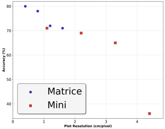
Figure 5.
Impact of image resolution on detection accuracy for two sensor platforms (Matrice and Mini). Detection accuracy declined sharply at resolutions coarser than 3.3 cm/pixel, underscoring the importance of sub-centimeter spatial resolution for reliable debris identification. The pattern was consistent across platforms, highlighting resolution as the dominant factor over sensor type.
The observed relationship between spatial resolution and detection accuracy can be attributed to several mechanisms. Higher resolution (0.4–1 cm) imagery preserves critical feature details and edge definition necessary for precise object boundary delineation, particularly important for distinguishing small debris items (3–25 cm) from similar-looking natural features. As resolution decreases, the ability to differentiate debris from background elements diminishes significantly, explaining the sharp accuracy decline observed at resolutions coarser than 3.3 cm. This relationship was consistent across both sensor platforms, confirming resolution itself, rather than sensor characteristics, was the primary determinant of detection performance. Achieving the optimal sub-centimeter resolution requires lower flight altitudes, creating significant operational trade-offs between detection accuracy and survey coverage efficiency.
3.3. Debris Distribution in Encampment Versus Non-Encampment Areas
Debris was highly concentrated in the encampment (Figure 6). The total area covered by debris represents a small fraction of the overall study area (56.66 m2 out of 2175.66 m2, or 2.6%), and the encampment has more than half (51%) of the total debris (Table 9). The higher debris concentration in encampments is further corroborated by the map comparing ground survey data with the DL debris map (Figure 6). The model underestimates debris quantity in some areas with high trash density, which could be partially attributed to overlapping debris. The high debris concentration in encampments suggests the potential for targeted cleanup efforts. There is a need for exploring solutions to assist unsheltered populations, such as frequent cleanups or providing waste receptacles.
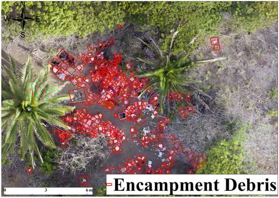
Figure 6.
Encampment detection results from UAV survey of Mission Valley Preserve. San Diego, California. Map shows detailed view of model detection results (red polygons) within the encampment area.
Table 9.
Distribution of debris across various land use types.
4. Discussion
This study highlights the potential of UAV-based deep learning for detecting anthropogenic debris in complex floodplains, with Cascade R-CNN outperforming other models. However, model performance may vary across different geographic and environmental conditions. We discuss three critical aspects: generalizability across landscapes, technical and environmental limitations, and protocols for broader validation. These factors are vital for scaling automated debris detection beyond localized deployments.
4.1. Model Performance and Generalizability Assessment
The potential of deep learning for anthropogenic debris detection was demonstrated using imagery collected by a UAV. Among the five approaches evaluated, the Cascade R-CNN model exhibited the highest accuracy across all image plots (Table 5, Figure S1), achieving greater than 65% for all plots, which agrees with previously reported accuracies exceeding 75% in similar applications of R-CNN [,,,,,]. The superior performance of Cascade R-CNN can be attributed to its multi-stage architecture, which progressively refines detections through an iterative process with increasingly strict Intersection over union (IoU) thresholds. This approach is particularly effective in complex floodplain environments where debris objects often overlap or are partially obscured by vegetation.
The success of the multi-stage refinement approach aligns with findings from other challenging environmental detection tasks. Similar progressive refinement architectures have proven effective in surface defect detection scenarios [] and complex imaging conditions [], suggesting that this architecture type is particularly well-suited for environmental monitoring applications where objects may be partially obscured or embedded in complex backgrounds.
While our model performed well within our study sites, the critical question of generalizability across different topographical and environmental conditions requires consideration. Our analysis reveals both the potential and limitations of the proposed method’s universal applicability. To evaluate generalizability, we conducted tests using imagery collected with different solar geometries (early morning versus midday), illumination conditions (sunny versus overcast), topographic settings (flat floodplains versus sloped canyon walls), and vegetation conditions (bare soil, herbaceous vegetation, and dense vegetation). We then conducted tests by applying the trained model to image subsets representing these environmental conditions and evaluating with the same metrics applied elsewhere in our analysis. The results revealed notable performance variations: model accuracy decreased by approximately 12% when applied to images captured under significantly different lighting conditions (early morning versus midday), by 15% in areas with vegetation types not well-represented in the training data, with dense shadows causing the most significant impact (18% accuracy reduction) and areas with unusual ground textures resulting in 14% accuracy reduction.
Our study encompassed two distinct environmental contexts: Mission Valley Preserve (MVP) with mixed vegetation and active encampments, and Alvarado Creek (AC) with minimal vegetation and scattered litter. The model showed varying performance across these sites (Table 5), with MVP October 2022 achieving the highest accuracy (0.93) and MVP February 2022 showing more modest performance (0.63). This variation demonstrates that even within the same watershed, environmental conditions significantly influence detection performance.
Based on our findings, a given method’s performance in other conditions would likely depend on several critical factors: terrain complexity (flatter terrain with minimal elevation changes should yield better results than steep, varied topography), vegetation density (areas with sparse to moderate vegetation coverage would be more suitable than densely forested regions), surface homogeneity (locations with uniform ground cover would facilitate better debris discrimination), and climate conditions (stable lighting conditions and minimal atmospheric interference would optimize performance).
Several factors emerged as critical determinants of model transferability: vegetation complexity (dense woody vegetation and palm tree coverage reduced detection accuracy, while bare soil and herbaceous vegetation showed better performance), lighting conditions (early morning and late afternoon imaging created shadows that significantly impacted detection capabilities), ground texture variability (areas with complex surface textures presented greater challenges for debris discrimination), and debris spatial distribution patterns (highly concentrated debris showed different detection patterns compared to scattered litter).
4.2. Technical Limitations and Environmental Constraints
One significant limitation was the inherent complexity of the floodplain environment compared to controlled settings used in previous studies [,]. Uneven terrain, overlapping debris, vegetation and varying lighting conditions presented challenges for the model to extract features and learn during training. These complexities echo similar challenges found in other domains. Wang et al. [] addressed challenges in unsupervised person re-identification through adaptive information supplementation and foreground enhancement, which parallels our approach of adaptively enhancing foreground debris features from complex backgrounds.
Spatial resolution was a critical factor for influencing detection accuracy and the method’s applicability across different environments. For the Matrice, accuracy remained relatively high (71% to 80%) across spatial resolutions from 0.40 cm to 1.60 cm. With the Mini, accuracy showed a gradual decline from 71% at 1.10 cm resolution to 36% at 4.40 cm resolution, with a notable decrease in performance at resolutions coarser than 3.30 cm. This resolution requirement has significant implications for universal applicability: operational constraints (achieving sub-centimeter resolution necessitates low-altitude flights, limiting coverage area and increasing survey time), cost considerations (while expensive units can be used, the dominant control of resolution over accuracy suggests that cost-effective UAVs can achieve comparable results if flown at appropriate altitudes), and terrain accessibility (some topographical conditions may limit low-altitude flight options, affecting the method’s applicability). However, we used our maps to identify concentrations of trash rather than the absolute cover percentage, and the main absolute quantity of interest is the volume, which is determined from a regression between mapped area and volume; and systemic over-estimation of cover would be corrected in the volume-area regression.
The validation loss curves (Figures S2–S4) suggest potential overfitting to training data, which may limit generalizability across highly varied environments. This limitation represents a significant concern for universal applicability and could be addressed through expanded training datasets representing diverse debris scenarios and environmental conditions from multiple geographical regions.
4.3. Implications and Recommendations for Universal Application
Encampment trash exhibits greater spatial concentration of debris compared to scattered debris, potentially making it easier to map and target for cleanup efforts. About half of unmanaged waste originated from encampment areas, with the remaining half dispersed across the floodplain (Table 9). This finding highlights the connection between homelessness and environmental issues, similar to previous studies that identify unsheltered homelessness as an environmental justice issue [,]. The methodology’s ability to identify these patterns suggests potential applicability in other urban watersheds facing similar challenges.
To enhance the method’s universal applicability across different topographical conditions, we recommend a comprehensive approach that combines expanded multi-regional training datasets, domain adaptation techniques [], environmental metadata integration(terrain type, vegetation density, climate conditions), and ensemble modeling strategies tailored to specific site characteristics.
For operational deployment in new topographical conditions, we recommend a systematic validation approach involving environmental site characterization, representative ground reference validation, accuracy benchmarking against predefined thresholds, context-specific model optimization, and continuous performance monitoring with iterative refinement.
5. Conclusions
This study successfully demonstrated the potential of deep learning techniques combined with UAV imagery for automated debris detection in complex floodplain environments. Through comprehensive field surveys and systematic visual interpretation, we established robust ground reference data that enabled rigorous model evaluation and validation.
Our comparative analysis revealed that the Cascade R-CNN model, implemented through the MMDetection framework, consistently outperformed single-stage detection architectures across all image collection dates. The model’s superior performance can be attributed to its multi-stage architecture, which progressively refines detections through iterative processing. This approach proved particularly effective for detecting obscured or overlapping debris items that challenged single-pass detection models.
The model demonstrated strong predictive capability, achieving good correlation between ground reference data and predictions in plot-level validation for both debris count (r = 0.74) and volume density (r = 0.80). This level of accuracy provides a solid foundation for prioritizing cleanup efforts by identifying areas with elevated debris concentrations, thereby optimizing resource allocation for environmental management agencies.
Our analysis identified potential overfitting in the validation loss curves, which requires targeted mitigation strategies for robust model deployment. To address overfitting and improve model robustness, we recommend a combination of L1/L2 regularization [], architectural enhancements such as spatial dropout [], dataset expansion across diverse conditions [], refined transfer learning, and ensemble model implementation to average out biases [].
The debris distribution maps generated by our approach (Figure 7, Figure 8 and Figure 9) provide valuable insights for cleanup agencies, enabling strategic planning and efficient resource allocation. These maps effectively identify trash hotspots and facilitate targeted intervention strategies, demonstrating the practical utility of automated debris detection systems.
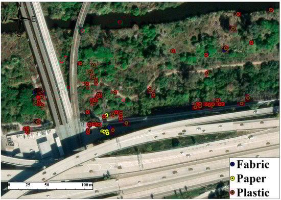
Figure 7.
Spatial distribution and classification of anthropogenic debris across survey sites and time periods based on UAV image analysis. Mission Valley Preserve—February 2022. Detected debris types are color-coded by material, illustrating temporal variation in density and spatial clustering.
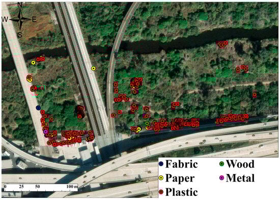
Figure 8.
Spatial distribution and classification of anthropogenic debris across survey sites and time periods based on UAV image analysis. Mission Valley Preserve—October 2022.
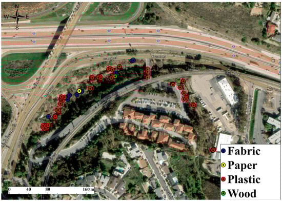
Figure 9.
Spatial distribution and classification of anthropogenic debris across survey sites and time periods based on UAV image analysis. Alvarado Creek—November 2023.
Our findings suggest that cost-effective UAVs can provide imagery at resolutions sufficient for comprehensive debris mapping, indicating potential for community-based and citizen science UAV programs to contribute to regional debris management initiatives. While this study focused on visible-light imagery, significant opportunities exist for enhancing detection capabilities through multispectral approaches. Near-infrared (NIR, 750–1400 nm) and short-wave infrared (SWIR, 1400–3000 nm) bands offer promising advantages for anthropogenic debris identification. NIR imagery could improve plastic detection by exploiting additional spectral contrast with soil and vegetation background, while SWIR bands can distinguish some polymer types on the basis of characteristic absorption features []. The spectral features could enable detection of debris items that are visually like their backgrounds in RGB imagery.
Additional research priorities include: (1) evaluating model generalizability across diverse environments and datasets, (2) assessing performance with lower spatial resolution imagery (>10 cm) with additional bands in the SWIR, (3) developing capabilities for material and plastic type classification, and (4) integrating thermal infrared sensors for enhanced early morning detection when temperature contrasts between anthropogenic and natural materials may be maximized.
This research contributes to advancing automated environmental monitoring capabilities and provides a scalable framework for debris management in flood-prone areas. The demonstrated effectiveness of UAV-based detection systems, combined with deep learning approaches, offers a practical solution for addressing the growing challenge of anthropogenic debris in natural environments. The methodology developed here can be adapted and scaled to support broader environmental conservation efforts and inform policy decisions regarding waste management and flood debris mitigation.
Supplementary Materials
The following supporting information can be downloaded at: https://www.mdpi.com/article/10.3390/rs17132172/s1, Figure S1: Spatial distribution of ground reference plots used for model training and validation across survey locations and periods. Mission Valley Preserve—February 2022. Plot locations were chosen to capture a variety of debris types, vegetation conditions, and encampment presence to ensure diverse training inputs and robust validation coverage; Figure S2: Spatial distribution of ground reference plots used for model training and validation across survey locations and periods. Mission Valley Preserve—October 2022; Figure S3: Spatial distribution of ground reference plots used for model training and validation across survey locations and periods. Alvarado Creek—November 2023; Figure S4: Detection results from the MMDetection model applied to ground plots at Mission Valley Preserve. (a) Detection output from the 18 February 2022, survey. (b) Detection output from the 29 October 2022, survey. Red boxes indicate predicted debris locations; Blue boxes indicate instances the model failed to predict debris; Figure S5: Training and validation loss curves for four deep learning models (DetReg, SSD, RetinaNet, Faster R-CNN) and one ensemble model (MMDetection) on the 5 × 10 m plot from the February 2022 Mission Valley Preserve survey. (a) Loss curves for DetReg, SSD, RetinaNet, and Faster R-CNN. (b) Loss curve for the MMDetection model using the Cascade R-CNN architecture; Figure S6: Training and validation loss curves for five models on the 5 × 15 m plot from the October 2022 Mission Valley Preserve survey. (a) DetReg, SSD, RetinaNet, and Faster R-CNN models. (b) MMDetection with Cascade R-CNN; Figure S7: Loss curves showing model training behavior for the Alvarado Creek site. (a) DetReg, SSD, RetinaNet, and Faster R-CNN models. (b) MMDetection model. Loss is plotted against number of training epochs; Figure S8: Impact of UAV flight altitude and corresponding image resolution on debris detection accuracy at the parking lot plot. Results are shown for both UAV platforms: (a–d) DJI Mini 2 at altitudes of 100 ft, 200 ft, 300 ft, and 400 ft, respectively; and (e–h) DJI Matrice 300 at matching altitudes. Detection performance declines noticeably with increasing altitude due to reduced spatial resolution, particularly beyond 300 ft; Figure S9: Impact of UAV flight altitude and corresponding image resolution on debris detection accuracy at the floodplain plot. Results are shown for both UAV platforms: (a–d) DJI Mini 2 at altitudes of 100 ft, 200 ft, 300 ft, and 400 ft, respectively; and (e–h) DJI Matrice 300 at matching altitudes. Detection performance declines noticeably with increasing altitude due to reduced spatial resolution, particularly beyond 300 ft.
Author Contributions
Conceptualization, T.B., D.S. and P.J.; methodology, P.J.; software, P.J.; validation, P.J.; formal analysis, P.J.; investigation, T.B., H.M. and P.J.; resources, L.C. and P.J.; data curation, L.C., S.H. and P.J.; writing—original draft preparation, P.J.; writing—review and editing, T.B. and D.S.; visualization, P.J., T.B. and D.S.; supervision, T.B. and H.M.; project administration, T.B. and H.M.; funding acquisition, H.M. and T.B. All authors have read and agreed to the published version of the manuscript.
Funding
Funding was provided by the National Oceanic and Atmospheric Administration (NOAA) Marine Debris Project [NA21NOS9990109]. The San Diego River Park Foundation provided significant logistical support in the field and participated in field data collection. The results of this project, as well as any view expressed herein, are those of the authors and do not necessarily reflect the views of NOAA. D.S. gratefully acknowledges funding from the NASA Remote Sensing of Water Quality Program (Grant #80NSSC22K0907) and the NASA Applications-Oriented Augmentations for Research and Analysis Program (Grant #80NSSC23K1460), as well as the USDA NIFA Sustainable Agroecosystems Program (Grant #2022-67019-36397), the NASA EMIT Science and Applications Team (Grant #80NSSC24K0861), the NASA Commercial Smallsat Data Analysis Program (Grant #80NSSC24K0052), and the NSF Signals in the Soil Program (Award #2226649).
Data Availability Statement
The datasets used in the current study are available (https://doi.org/10.5281/zenodo.15304459).
Conflicts of Interest
The authors declare no conflicts of interest.
References
- Siddiqua, A.; Hahladakis, J.N.; Al-Attiya, W.A.K.A. An Overview of the Environmental Pollution and Health Effects Associated with Waste Landfilling and Open Dumping. Environ. Sci. Pollut. Res. 2022, 29, 58514–58536. [Google Scholar] [CrossRef]
- Tuholske, C.; Halpern, B.S.; Blasco, G.; Villasenor, J.C.; Frazier, M.; Caylor, K. Mapping Global Inputs and Impacts from of Human Sewage in Coastal Ecosystems. PLoS ONE 2021, 16, e0258898. [Google Scholar] [CrossRef]
- Abubakar, I.R.; Maniruzzaman, K.M.; Dano, U.L.; AlShihri, F.S.; AlShammari, M.S.; Ahmed, S.M.S.; Al-Gehlani, W.A.G.; Alrawaf, T.I. Environmental Sustainability Impacts of Solid Waste Management Practices in the Global South. Int. J. Environ. Res. Public Health 2022, 19, 12717. [Google Scholar] [CrossRef]
- Lincoln, S.; Andrews, B.; Birchenough, S.N.R.; Chowdhury, P.; Engelhard, G.H.; Harrod, O.; Pinnegar, J.K.; Townhill, B.L. Marine Litter and Climate Change: Inextricably Connected Threats to the World’s Oceans. Sci. Total Environ. 2022, 837, 155709. [Google Scholar] [CrossRef]
- Gerrity, D.; Papp, K.; Dickenson, E.; Ejjada, M.; Marti, E.; Quinones, O.; Sarria, M.; Thompson, K.; Trenholm, R.A. Characterizing the Chemical and Microbial Fingerprint of Unsheltered Homelessness in an Urban Watershed. Sci. Total Environ. 2022, 840, 156714. [Google Scholar] [CrossRef]
- Marie, A. An Assessment of Mitigation Strategies to Address Environmental Impacts of Homeless Encampments. Master’s Thesis, California State University, Long Beach, CA, USA, 2019. [Google Scholar]
- Langat, P.K.; Kumar, L.; Koech, R. Monitoring River Channel Dynamics Using Remote Sensing and GIS Techniques. Geomorphology 2019, 325, 92–102. [Google Scholar] [CrossRef]
- Topouzelis, K.; Papageorgiou, D.; Karagaitanakis, A.; Papakonstantinou, A.; Ballesteros, M.A. Remote Sensing of Sea Surface Artificial Floating Plastic Targets with Sentinel-2 and Unmanned Aerial Systems (Plastic Litter Project 2019). Remote Sens. 2020, 12, 2013. [Google Scholar] [CrossRef]
- Kylili, K.; Kyriakides, I.; Artusi, A.; Hadjistassou, C. Identifying Floating Plastic Marine Debris Using a Deep Learning Approach. Environ. Sci. Pollut. Res. 2019, 26, 17091–17099. [Google Scholar] [CrossRef]
- Benali Amjoud, A.; Amrouch, M. Convolutional Neural Networks Backbones for Object Detection. In Image and Signal Processing, Proceedings of the 9th International Conference, ICISP 2020, Marrakesh, Morocco, 4–6 June 2020; Lecture Notes in Computer Science (Including Subseries Lecture Notes in Artificial Intelligence and Lecture Notes in Bioinformatics); Springer: Berlin/Heidelberg, Germany, 2020; Volume 12119 LNCS, pp. 282–289. [Google Scholar]
- Zhang, C.; Zhang, X.; Tu, D.; Wang, Y. Small Object Detection Using Deep Convolutional Networks: Applied to Garbage Detection System. J. Electron. Imaging 2021, 30, 043013. [Google Scholar] [CrossRef]
- Kussul, N.; Lavreniuk, M.; Skakun, S.; Shelestov, A. Deep Learning Classification of Land Cover and Crop Types Using Remote Sensing Data. IEEE Geosci. Remote Sens. Lett. 2017, 14, 778–782. [Google Scholar] [CrossRef]
- Mittal, G.; Yagnik, K.B.; Garg, M.; Krishnan, N.C. SpotGarbage: Smartphone App to Detect Garbage Using Deep Learning. In Proceedings of the UbiComp 2016—Proceedings of the 2016 ACM International Joint Conference on Pervasive and Ubiquitous Computing, Heidelberg, Germany, 12 September 2016; Association for Computing Machinery, Inc.: New York, NY, USA; pp. 940–945. [Google Scholar]
- Chai, B.; Nie, X.; Zhou, Q.; Zhou, X. Enhanced Cascade R-CNN for Multi-Scale Object Detection in Dense Scenes from SAR Images. IEEE Sens. J. 2024, 24, 20143–20153. [Google Scholar] [CrossRef]
- Li, M.T.; Lee, S.H. A Study on Small Pest Detection Based on a CascadeR-CNN-Swin Model. Comput. Mater. Contin. 2022, 72, 6155–6165. [Google Scholar] [CrossRef]
- Cai, Q.; Pan, Y.; Yao, T.; Mei, T. 3D Cascade RCNN: High Quality Object Detection in Point Clouds. IEEE Trans. Image Process. 2022, 31, 5706–5719. [Google Scholar] [CrossRef]
- Wu, L.; Chen, S.; Liang, C. Target Detection of Marine Ships Based on a Cascade RCNN. In Proceedings of the 2021 International Conference on Advanced Technologies and Applications of Modern Industry (ATAMI 2021), Wuhan, China, 19–21 November 2021; IOP Publishing Ltd.: Bristol, UK, 2022; Volume 2185. [Google Scholar]
- Li, P.; Tao, H.; Zhou, H.; Zhou, P.; Deng, Y. Enhanced Multiview Attention Network with Random Interpolation Resize for Few-Shot Surface Defect Detection. Multimed. Syst. 2025, 31, 36. [Google Scholar] [CrossRef]
- Chen, X.; Tao, H.; Zhou, H.; Zhou, P.; Deng, Y. Hierarchical and Progressive Learning with Key Point Sensitive Loss for Sonar Image Classification. Multimed. Syst. 2024, 30, 380. [Google Scholar] [CrossRef]
- Helber, P.; Bischke, B.; Dengel, A.; Borth, D. Eurosat: A Novel Dataset and Deep Learning Benchmark for Land Use and Land Cover Classification. IEEE J. Sel. Top. Appl. Earth Obs. Remote Sens. 2019, 12, 2217–2226. [Google Scholar] [CrossRef]
- Cardiel-Ortega, J.J.; Baeza-Serrato, R. Failure Mode and Effect Analysis with a Fuzzy Logic Approach. Systems 2023, 11, 348. [Google Scholar] [CrossRef]
- Martin, C.; Parkes, S.; Zhang, Q.; Zhang, X.; McCabe, M.F.; Duarte, C.M. Use of Unmanned Aerial Vehicles for Efficient Beach Litter Monitoring. Mar. Pollut. Bull. 2018, 131, 662–673. [Google Scholar] [CrossRef]
- Castellanos-Galindo, G.A.; Casella, E.; Mejía-Rentería, J.C.; Rovere, A. Habitat Mapping of Remote Coasts: Evaluating the Usefulness of Lightweight Unmanned Aerial Vehicles for Conservation and Monitoring. Biol. Conserv. 2019, 239, 108282. [Google Scholar] [CrossRef]
- Andriolo, U.; Topouzelis, K.; van Emmerik, T.H.M.; Papakonstantinou, A.; Monteiro, J.G.; Isobe, A.; Hidaka, M.; Kako, S.; Kataoka, T.; Gonçalves, G. Drones for Litter Monitoring on Coasts and Rivers: Suitable Flight Altitude and Image Resolution. Mar. Pollut. Bull. 2023, 195, 115521. [Google Scholar] [CrossRef]
- Fallati, L.; Polidori, A.; Salvatore, C.; Saponari, L.; Savini, A.; Galli, P. Anthropogenic Marine Debris Assessment with Unmanned Aerial Vehicle Imagery and Deep Learning: A Case Study along the Beaches of the Republic of Maldives. Sci. Total Environ. 2019, 693, 133581. [Google Scholar] [CrossRef]
- Maharjan, N.; Miyazaki, H.; Pati, B.M.; Dailey, M.N.; Shrestha, S.; Nakamura, T. Detection of River Plastic Using UAV Sensor Data and Deep Learning. Remote Sens. 2022, 14, 3049. [Google Scholar] [CrossRef]
- Garcia-Garin, O.; Monleón-Getino, T.; López-Brosa, P.; Borrell, A.; Aguilar, A.; Borja-Robalino, R.; Cardona, L.; Vighi, M. Automatic Detection and Quantification of Floating Marine Macro-Litter in Aerial Images: Introducing a Novel Deep Learning Approach Connected to a Web Application in R. Environ. Pollut. 2021, 273, 116490. [Google Scholar] [CrossRef]
- Wu, Z.; Yi, L.; Zhang, G. Uncertainty Analysis of Object Location in Multi-Source Remote Sensing Imagery Classification. Int. J. Remote Sens. 2009, 30, 5473–5487. [Google Scholar] [CrossRef]
- He, L.; Valocchi, A.J.; Duarte, C.A. A Transient Global-Local Generalized FEM for Parabolic and Hyperbolic PDEs with Multi-Space/Time Scales. J. Comput. Phys. 2023, 488, 112179. [Google Scholar] [CrossRef]
- Stein, T.; Peelen, M.V. Object Detection in Natural Scenes: Independent Effects of Spatial and Category-Based Attention. Atten. Percept. Psychophys. 2017, 79, 738–752. [Google Scholar] [CrossRef]
- Dettinger, M.D.; Ralph, F.M.; Das, T.; Neiman, P.J.; Cayan, D.R. Atmospheric Rivers, Floods and the Water Resources of California. Water Switz. 2011, 3, 445–478. [Google Scholar] [CrossRef]
- Ahn, J.H.; Grant, S.B.; Surbeck, C.Q.; Digiacomo, P.M.; Nezlin, N.P.; Jiang, S. Coastal Water Quality Impact of Stormwater Runoff from an Urban Watershed in Southern California. Environ. Sci. Technol. 2005, 39, 5940–5953. [Google Scholar] [CrossRef]
- Kamel, O.; Aboelenien, N.; Amin, K.; Semary, N. An Automated Contrast Enhancement Technique for Remote Sensed Images. Int. J. Comput. Inf. 2024, 11, 1–16. [Google Scholar] [CrossRef]
- Lin, T.Y.; Goyal, P.; Girshick, R.; He, K.; Dollar, P. Focal Loss for Dense Object Detection. In Proceedings of the IEEE International Conference on Computer Vision, Venice, Italy, 22–29 December 2017; Institute of Electrical and Electronics Engineers Inc.: New York, NY, USA, 2017; Volume 2017, pp. 2999–3007. [Google Scholar]
- Li, Y.; He, L.; Zhang, M.; Cheng, Z.; Liu, W.; Wu, Z. Improving the Performance of the Single Shot Multibox Detector for Steel Surface Defects with Context Fusion and Feature Refinement. Electron. Switz. 2023, 12, 2440. [Google Scholar] [CrossRef]
- Ren, S.; He, K.; Girshick, R.; Sun, J. Faster R-CNN: Towards Real-Time Object Detection with Region Proposal Networks. IEEE Trans. Pattern Anal. Mach. Intell. 2017, 39, 1137–1149. [Google Scholar] [CrossRef]
- Feng, Y.; You, Y.; Tian, J.; Meng, G. OEGR-DETR: A Novel Detection Transformer Based on Orientation Enhancement and Group Relations for SAR Object Detection. Remote Sens. 2024, 16, 106. [Google Scholar] [CrossRef]
- Cai, Z.; Vasconcelos, N. Cascade R-CNN: Delving into High Quality Object Detection. In Proceedings of the IEEE Computer Society Conference on Computer Vision and Pattern Recognition, Salt Lake City, UT, USA, 18–23 June 2018; IEEE Computer Society: Washington, DC, USA, 2018; pp. 6154–6162. [Google Scholar]
- Wang, L.; Zeng, X.; Yang, H.; Lv, X.; Guo, F.; Shi, Y.; Hanif, A. Investigation and Application of Fractal Theory in Cement-Based Materials: A Review. Fractal Fract. 2021, 5, 247. [Google Scholar] [CrossRef]
- Kraft, M.; Piechocki, M.; Ptak, B.; Walas, K. Autonomous, Onboard Vision-Based Trash and Litter Detection in Low Altitude Aerial Images Collected by an Unmanned Aerial Vehicle. Remote Sens. 2021, 13, 965. [Google Scholar] [CrossRef]
- Morgan, G.R.; Wang, C.; Li, Z.; Schill, S.R.; Morgan, D.R. Deep Learning of High-Resolution Aerial Imagery for Coastal Marsh Change Detection: A Comparative Study. ISPRS Int. J. Geo-Inf. 2022, 11, 100. [Google Scholar] [CrossRef]
- Abd-Elrahman, A.; Britt, K.; Liu, T. Deep Learning Classification of High-Resolution Drone Images Using the ArcGIS Pro Software. EDIS 2021, 2021. [Google Scholar] [CrossRef]
- Hennig, S. Orchard Meadow Trees: Tree Detection Using Deep Learning in ArcGIS Pro. GI_Forum 2021, 9, 82–93. [Google Scholar] [CrossRef]
- Khalid, N.; Shahrol, N.A. Evaluation the Accuracy of Oil Palm Tree Detection Using Deep Learning and Support Vector Machine Classifiers. In Proceedings of the 8th International Conference on Geomatics and Geospatial Technology (GGT 2022), Online, 25–26 May 2022; Institute of Physics: London, UK, 2022; Volume 1051. [Google Scholar]
- Majchrowska, S.; Mikołajczyk, A.; Ferlin, M.; Klawikowska, Z.; Plantykow, M.A.; Kwasigroch, A.; Majek, K. Deep Learning-Based Waste Detection in Natural and Urban Environments. Waste Manag. 2022, 138, 274–284. [Google Scholar] [CrossRef]
- Wang, Q.; Huang, Z.; Fan, H.; Fu, S.; Tang, Y. Unsupervised Person Re-Identification Based on Adaptive Information Supplementation and Foreground Enhancement. IET Image Process. 2024, 18, 4680–4694. [Google Scholar] [CrossRef]
- Verbyla, M.E.; Calderon, J.S.; Flanigan, S.; Garcia, M.; Gersberg, R.; Kinoshita, A.M.; Mladenov, N.; Pinongcos, F.; Welsh, M. An Assessment of Ambient Water Quality and Challenges with Access to Water and Sanitation Services for Individuals Experiencing Homelessness in Riverine Encampments. Environ. Eng. Sci. 2021, 38, 389–401. [Google Scholar] [CrossRef]
- Singhal, P.; Walambe, R.; Ramanna, S.; Kotecha, K. Domain Adaptation: Challenges, Methods, Datasets, and Applications. IEEE Access 2023, 11, 6973–7020. [Google Scholar] [CrossRef]
- Goodfellow, I.; Bengio, Y.; Courville, A. Deep Learning; The MIT Press: Cambridge, MA, USA, 2016. [Google Scholar]
- Mikołajczyk, A.; Grochowski, M. Data augmentation for improving deep learning in image classification problem. In Proceedings of the 2018 International Interdisciplinary PhD Workshop (IIPhDW), Świnouście, Poland, 9–12 May 2018; pp. 117–122. [Google Scholar] [CrossRef]
- Ganaie, M.A.; Hu, M.; Malik, A.K.; Tanveer, M.; Suganthan, P.N. Ensemble Deep Learning: A Review. Eng. Appl. Artif. Intell. 2022, 115, 105151. [Google Scholar] [CrossRef]
- Aguilar, E.; Sousa, D.; Uhrin, A.; Gudino-Elizondo, N.; Biggs, T. Mapping terrestrial macroplastics and polymer-coated materials in an urban watershed using WorldView-3 and laboratory reflectance spectroscopy. Environ. Monit. Assess. 2025, in press. [CrossRef]
Disclaimer/Publisher’s Note: The statements, opinions and data contained in all publications are solely those of the individual author(s) and contributor(s) and not of MDPI and/or the editor(s). MDPI and/or the editor(s) disclaim responsibility for any injury to people or property resulting from any ideas, methods, instructions or products referred to in the content. |
© 2025 by the authors. Licensee MDPI, Basel, Switzerland. This article is an open access article distributed under the terms and conditions of the Creative Commons Attribution (CC BY) license (https://creativecommons.org/licenses/by/4.0/).