Providing Enhanced Insights into Groundwater Exchange Patterns through Downscaled GRACE Data

Abstract

The measurement of groundwater exchange between neighboring regions is a critical topic in water resource management and can usually be achieved through a combination of field investigations and the use of groundwater flow models. In this study, we employed the water balance and Darcy’s law methods, utilizing downscaled Gravity Recovery and Climate Experiment (GRACE) and GRACE-Follow On (GRACE-FO) data to assess groundwater exchange patterns in the Beijing-Tianjin-Hebei (BTH) region of China. Additionally, we determined the contributions of human activities and climate factors to the observed variations via residual analysis. The results revealed a consistent decrease in groundwater storage in the study area since 2008, especially in the spring and summer months. The groundwater exchange rates calculated by 1° and 0.05° groundwater storage anomalies (GWSAs) were basically consistent, and the downscaled GWSAs could better reflect the small-scale groundwater exchange characteristics. The groundwater exchange rate showed a decreasing trend from the Piedmont plain to the coastal areas. A notable trend of declining groundwater exchange between the Taihang Mountains and Piedmont plains was observed, and the downward trend gradually intensified from north to south between 2003 and 2007. After 2008, there was an increasing trend, and coastal areas exhibited the smallest amount of groundwater exchange. Human activities emerged as the predominant factor accounting for more than 90.9% of the overall reduction in groundwater storage, while climate change imposed a minimal influence on groundwater storage variations. The insights obtained in this study hold significant implications for groundwater resource planning and management in the region.

1. Introduction

Groundwater represents a vital freshwater resource that plays a pivotal role in facilitating sustainable human development and preserving ecosystems. However, compared to other water sources, such as rivers, soil, and lakes, our understanding of groundwater availability remains limited. Aquifers experience gradual changes and follow extended replenishment and discharge cycles, constituting a dynamic equilibrium process between recharge and discharge. When subjected to human activities, both the replenishment and discharge rates of groundwater are affected, particularly in densely irrigated agricultural regions [1,2]. When discharge exceeds recharge, a series of ecological and geological challenges can occur [3,4]. Consequently, analyzing the spatiotemporal fluctuations in groundwater storage (GWS) within aquifers is necessary for effective water resource planning and management.

Since its launch in 2002, the Gravity Recovery and Climate Experiment (GRACE) has emerged as a valuable and precise tool for monitoring significant shifts in terrestrial water storage on a large scale [5,6,7]. It is an invaluable resource when on-site groundwater monitoring wells are unavailable or as a complementary component to existing groundwater monitoring networks. For instance, in Northwest India [6], the U.S. High Plains and Central Valley in California [8,9], the Colorado River Basin [10], Australia [11,12], and the Middle East [13]. Especially in North China, numerous studies [14,15,16,17,18,19] have focused on explaining the depletion of groundwater resources, as well as the effects of the South-to-North Water Diversion Project on groundwater storage in the North China Plain [20,21,22]. As the timeline of GRACE monitoring data increases and data processing capabilities improve, there is a growing interest in employing statistical downscaling techniques (e.g., multiple regression [23], artificial neural networks [24], and machine learning [25]) or dynamic downscaling approaches, such as data assimilation [26] and hydrological models [27], to assess small-scale regional groundwater storage variations. In North China, Yin et al. [28] effectively employed statistical downscaling of GRACE-derived groundwater storage anomalies (GWSA) by incorporating evapotranspiration data in the North China Plain, yielding satisfactory results. We adopted a dynamic downscaling approach to downscale GRACE-derived GWSA data at a spatial resolution of 0.05° in the Beijing-Tianjin-Hebei (BTH) region by constructing a groundwater storage model and assessed the changes in groundwater storage between different regions [29].

Nonetheless, evaluating groundwater storage changes using GRACE data presents challenges due to the inclusion of total water variations within aquifers, making it difficult to separate the impacts of boundary fluxes on storage changes. Groundwater level monitoring offers more precise in situ data, enabling the estimation of groundwater exchange using Darcy’s law based on groundwater level contour maps [30]. However, economic constraints often result in an insufficient number of groundwater level monitoring wells with inadequate spatial distributions for reliably representing groundwater exchange [31,32]. Numerical models, which offer considerable flexibility and predictive capabilities, can be used to characterize the groundwater environment, providing comprehensive and detailed insights into groundwater flow dynamics [30,31,32,33]. However, this approach necessitates accurate initial and boundary conditions, and imperfect input data could lead to inaccurate results [34,35]. In addition, groundwater exchange can be studied through diverse techniques, such as tracer tests [36,37,38], groundwater chemical analysis [39], and water balance or water cycle methodologies [40,41,42]. Another limitation of these approaches is that the total surface area undergoing recharge must be estimated to calculate regional recharge rates. Yin et al. [43] proposed a method that leverages GRACE data, water balance calculations, and Darcy’s law to assess groundwater exchange along different boundaries in the Heihe River Basin in China, producing reliable results. This method is simple and efficient because GRACE data are readily accessible without limitations related to time and space. However, the study of Yin et al. [43] exhibits several limitations, including the coarse resolution of the GRACE products used, as their analysis of groundwater exchange was based on 1° GRACE data, which are less suitable for small-scale applications. Additionally, they did not account for the data gap between GRACE and GRACE-Follow On (GRACE-FO) data, and the utilized data time series were relatively short.

The North China region is the world’s largest groundwater depletion zone, resulting in ecological and environmental challenges such as land subsidence and seawater intrusion [44,45]. Several key factors impact groundwater recharge and the discharge flux in the North China region, including groundwater extraction, precipitation, upstream inflow from hilly regions, and interregional water transfers [46]. Mountain front lateral flow is a significant source of recharge, with an impact second only to that of groundwater extraction in North China, but this process is not well understood or quantified [47,48]. In light of the complex human activities in this region, it is important to establish quantitative methodologies for understanding groundwater exchange and investigating groundwater dynamics across different areas. Therefore, this study begins by obtaining downscaled GRACE data and then applying the method of Yin et al. [43] for assessing groundwater exchange in the BTH region, with a focus on the interactions between mountainous regions, plains, coastal areas, and different administrative zones. Furthermore, we analyze the factors influencing groundwater storage exchange and quantitatively assess the contributions of both human and meteorological factors to groundwater storage changes. The research findings hold significant implications for the comprehensive management of overexploited groundwater resources in the BTH region.

2. Materials

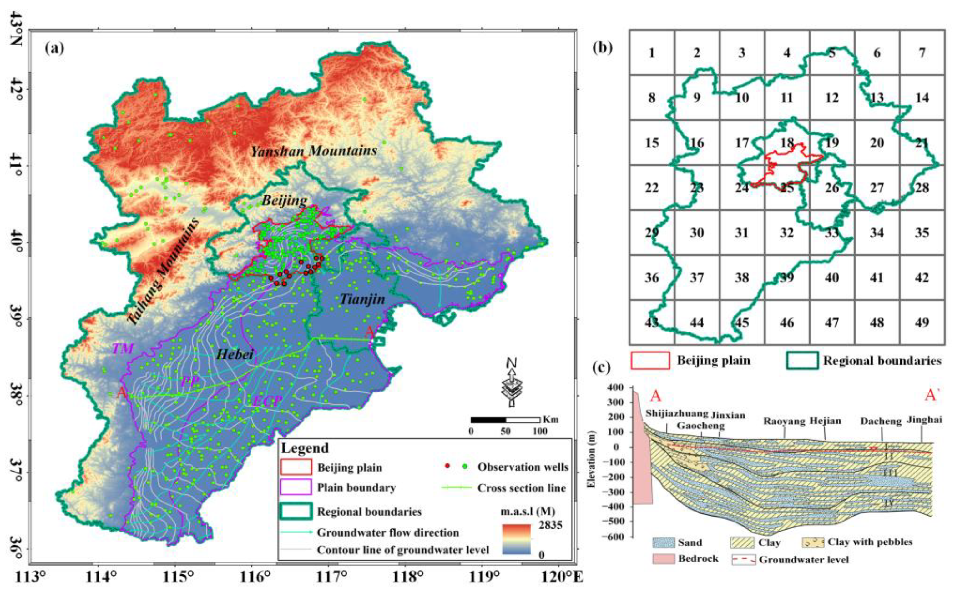
2.1. Study Area

The Beijing-Tianjin-Hebei region is situated in the North China Plain and extends from approximately 36°01′ to 42°35′ and from 113°29′ to 119°58′, covering a total area of approximately 218,000 km² (Figure 1a). This region exhibits a gradual topographic transition from the northwesterly Yanshan-Taihang Mountains system to the southeastern plains, revealing distinctive elevation characteristics from high to low. Geographically, the region can be divided into two main zones: the mountainous area and the BHT plain. Within the BTH Plain, there are further subdivisions, including the Piedmont plain (PP) and the east–central plain (ECP). The Beijing Plain is located at the intersection of the Yanshan and Taihang Mountains (YM and TM, respectively) ranges, as shown in Figure 1a.

In the study area, groundwater is influenced by various factors, including deposition, topographical features and human activities. In the Piedmont zone, the Quaternary aquifer comprises alluvial and colluvial deposits characterized by cohesive soil mixed with gravel. These deposits are often poorly sorted and contain local aquifers. Moving from the Piedmont zone to the plain, the aquifer becomes multilayered, with the lithology changing from cobbles to gravel and ultimately to multilayered sand deposits. In some single-layered structures, clay layers enclose certain areas, forming lens-shaped bodies. These deposits can be categorized into four hydrostratigraphic units, as shown in Figure 1c. Deposits units (I and II) either directly or indirectly receive recharge from precipitation, creating favorable connections for intense vertical circulation, usually combined into a shallow groundwater system. In contrast, deposit types III and IV are confined aquifers with poor hydraulic conditions, resulting in a low hydraulic conductivity zone, usually combined into a deep groundwater system. Generally, the boundary between shallow and deep groundwater systems occurs at a burial depth of approximately 120 m, which are mutually independent yet interconnected [46]. The aquifers exhibit a gradual decrease in the estimated yield, decreasing from 3000–5000 m³/d in the Piedmont plains to 100–500 m³/d in the central and coastal plains.

The BTH region exhibits a semiarid continental monsoon climate and is primarily drained by the Luan River and Hai River systems. The annual average precipitation ranges from 500–600 mm, while the annual potential evaporation ranges from approximately 1100–2000 mm. To meet the water demands for economic and social development, the BTH region experienced water resource development and utilization, which peaked at 106%. Even after the completion of the South-to-North Water Diversion Project in 2014, 70% of the water resources remained overexploited, indicating severe overexploitation of the regional water resources. The water supply in the BTH region relies on groundwater, surface water, and other sources, such as reclaimed water and water transfers. As shown in Figure 2, groundwater extraction has significantly decreased in recent years due to stringent regulations. Between 2000 and 2021, the proportion of groundwater in the water supply decreased from more than 75% to 35%, while the proportion of surface water increased from 26% to 55%. The groundwater levels in the Beijing Plain reached their lowest value in 2014, while they gradually recovered with water source replacement from the South-to-North Water Diversion Project. Similarly, in the Hebei Plain, efforts to control groundwater overexploitation in the North China region have limited the rate of decrease in groundwater levels. In terms of water usage, agricultural water consumption decreased from 70% to 40% between 2000 and 2021, while water usage for ecological and environmental purposes has steadily increased in recent years.

2.2. Data Sources

2.2.1. Groundwater Storage Dataset

In our previous research, we introduced a numerical simulation technique aimed at downscaling GRACE-derived groundwater storage anomalies data, which resulted in the creation of the “Groundwater Storage Model”. This model parallels traditional groundwater flow numerical models in its core functionality; it too is fundamentally a numerical model. The distinct feature of our model lies in its simulation of groundwater storage rather than groundwater levels [29]. This method has been successfully applied to the BTH region and downscaled the spatial resolution of GWSAs from 1° to 0.05°. This downscaling process not only captured temporal variations consistent with those in the GRACE-derived GWSAs but also more precisely revealed spatial variations. For example, in a transect across a 1° grid before downscaling, the GRACE-derived GWSA is represented by homogenized pixels with a value of −34.46 cm EWH, while GWSA varied from −22.98 to −39.05 cm EWH in the transect after downscaling. Compared to that of the 1° GRACE-derived GWSAs, the average correlation coefficient (CC) between the downscaled GWSAs and in situ groundwater level measurements increased by 0.06, while the average root means square error (RMSE) decreased by 8.85%. For a more detailed presentation and validation of downscaled results, please refer to Sun et al. [29].

On the basis of our previous study, we utilized total water storage anomaly (TWSA) data from the Jet Propulsion Laboratory mass concentration blocks (JPL mascon), which is a simple linear interpolation method used to address data gaps in the GRACE product. While this approach is effective for short data gaps (1–2 months), it is unreliable for longer gaps, such as the approximately one-year gap between the GRACE and GRACE-FO missions [4,49]. Consequently, we did not present downscaled results for the period between July 2017 and May 2018 in our previous study.

The objective of this study was to assess groundwater exchange in the BTH region via a downscaled dataset for the period between 2003 and 2020. Downscaled GWSA data from July 2017 to May 2018 were estimated using the same dynamic downscaling methodology, with the boundary conditions derived from the previously reconstructed 1° TWSA dataset. Sun et al. [29,50] provided a comprehensive description of the principles of downscaling models. The datasets used, including rainfall, evapotranspiration, TWSA, soil moisture, and snow water equivalent data, can be obtained from the following link: https://figshare.com/articles/dataset/Downscaled_GWSA_dataset/20406309, accessed on 8 November 2023.

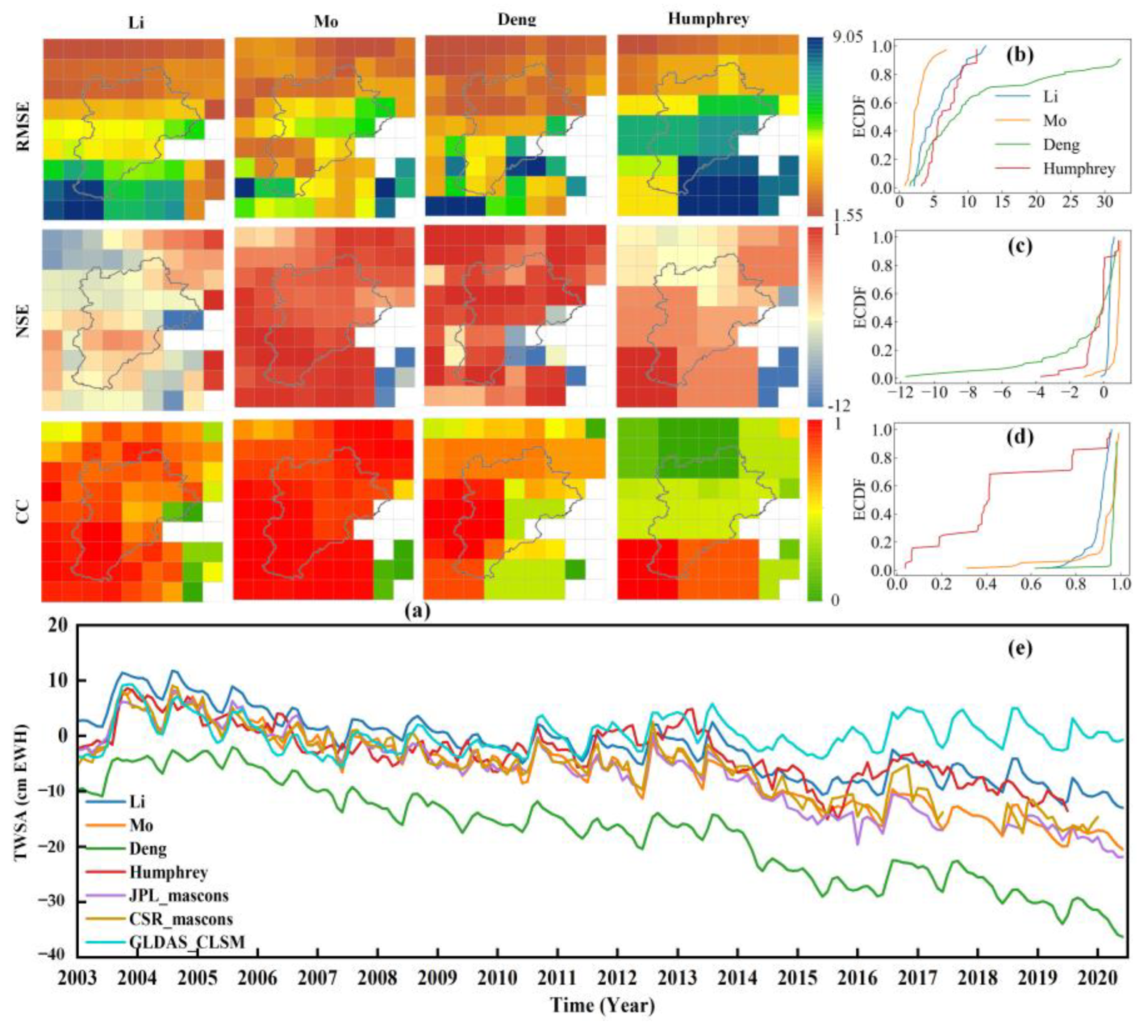
2.2.2. Comparison of the Reconstructions between the GRACE and GRACE-FO Data

The JPL and Center for Space Research of the University of Texas in Austin mascon dataset (CSR mascon) is widely employed for GRACE TWSA reconstruction. In contrast to spherical harmonics, mascon datasets offer a notable advantage in mitigating land-to-ocean signal leakage, leading to enhanced signal amplitudes. Additionally, geophysical data constraints are incorporated during processing, which necessitates minimal empirical postprocessing, thus increasing the user-friendliness for nongeodetic users [51]. Figure 3e reveals that both the JPL and CSR mascon datasets exhibit overall consistency in terms of trends and seasonal variations. However, the TWSA simulated by the Global Land Data Assimilation System Catchment Land Surface Model (GLDAS_CLSM), which neglects groundwater and surface water components as well as deep groundwater storage and human interventions, tends to underestimate groundwater storage changes [52].

Due to the target for our downscaling is the JPL mascon dataset, therefore, we compared four reconstructed datasets (referred to as Humphrey, Mo, Li, and Deng) from January 2003 to June 2017 with the JPL mascon data. The details and methodologies for these four reconstruction datasets are provided in

Table 1. Overview of different reconstruction data methods.

Source	Mo et al. (2022) [52]	Humphrey and Gudmundsson (2019) [53]	Deng et al. (2023) [54]	Li et al. (2021) [55]
Study area	Global	Global	Global	Global
Method	Bayesian convolutional neural network	A simple statistical model that considers the residence times of local TWS datapoints	Summation method, empirical orthogonal function bias correction, and multiple linear regression	Signal separation and detrending
GRACE data	JPL mascon	JPL mascon	JPL mascon	CSR mascon
Forcing data	Precipitation, temperature, cumulative water storage change, and ERA5L-derived TWSA	Precipitation and land temperature	Soil moisture, snow depth, precipitation, land temperature, and glacier mass change	Precipitation, land temperature, sea surface temperature, soil moisture, evaporation, runoff, and 17 other tele-connected climate indices
Time period	April 2002–December 2020	January 1901–July 2019	January 1981–June 2020	July 1979–June 2020
Spatial resolution	1° × 1°	0.5° × 0.5°	1° × 1°	0.5° × 0.5°

. The TWSA dataset of Humphrey et al. lacks seasonal cycles and information on the influence of human activities on terrestrial water storage, which are primarily driven by long-term precipitation trends, resulting in underestimation of groundwater storage changes [53]. Deng et al.’s TWSA data exhibit the highest correlation with the JPL mascon product data but also exhibit the highest median RMSE value of 7.2 cm for the equivalent water thickness (EWH) and a negative Nash–Sutcliffe efficiency coefficient (NSE) relative to the JPL mascon product. This difference can be attributed to the baseline deduction, calculated as the average value of each grid from January 1981 to June 2020 [54]. There is a significant difference between the CSR mascon dataset reconstructed by Li, which is significantly larger than the TWSA dataset provided by the CSR organization [55]. In contrast, Mo’s reconstructed TWSA data exhibited reasonable spatial consistency with the TWSA data provided by the JPL mascon dataset, accurately representing the TWSA from July 2017 to May 2018 when considering the overall regional average (Figure 3e) [52]. The median CC, RMSE, and NSE of the Mo dataset are 0.97, 2.16 cm, and 0.84, respectively. Furthermore, empirical cumulative distribution function analysis (Figure 3b–d) demonstrated that the quality of the reconstructed Mo data surpassed that of the other three datasets. Consequently, we employed Mo’s reconstructed TWSA data to bridge the data gap between the GRACE and GRACE-FO missions.

In this study, GRACE-derived GWSA is used as the Dirichlet boundary condition of the groundwater storage model. To address the differences between the reconstructed TWSA of each grid and that observed by the GRACE mission, as shown in Figure 3a, with the maximum RMSE between the reconstructed data of Mo and the JPL mascon data reaching 6.8 cm EWH and the minimum reaching 0.8 cm EWH, we adjusted Mo’s predicted TWSA for the period ranging from July 2017 to May 2018. This adjustment is based on the absolute errors observed during the validation periods established by Mo, ranging from April 2004 to June 2017 and June 2018 to December 2020. This correction enabled us to derive a continuous TWSA series by combining JPL mascon data (April 2002 to June 2017 and June 2018 to December 2020) and Mo’s reconstruction data (July 2017 to May 2018). Finally, the GWSA was computed by subtracting the soil moisture anomaly and snow water equivalent anomaly from the continuous TWSA. These GWSA values were then employed as boundary conditions in our groundwater storage model in conjunction with the actual observed values. Finally, we obtained a GWSA dataset from 2003 to 2020, with a 0.05° spatial resolution, through a downscaling process.

2.2.3. Ground-Based Measurements

In this study, monthly groundwater level data from 2003 to 2020 were analyzed to compare the fluctuations in groundwater storage and groundwater levels. Groundwater level data from 636 groundwater monitoring wells were obtained from public reports of the China Geological Environment Monitoring Institute, primarily located in the BTH region (Figure 1a). In this dataset, different observations have different starting times, and the periods of available data vary from station to station. Within the study area, despite the classification of deposits into four distinct types, aquifer types I and II are commonly aggregated to form a shallow groundwater system, and similarly, aquifer types III and IV are grouped to constitute a deep groundwater system. Those groundwater monitoring wells are categorized accordingly into ‘shallow’ and ‘deep’ wells. This classification extends to the groundwater flow fields, which are differentiated into shallow and deep layers. Consequently, for the purposes of this study, we postulated that groundwater levels within aquifer types I and II are equivalent, as are the water levels within aquifer types III and IV. Additionally, data from 185 groundwater monitoring wells were obtained from the Beijing Hydrological Station, mainly shallow groundwater level monitoring wells. These wells are mainly distributed in the Beijing Plain region. Groundwater level data within each 1° or 0.05° grid were obtained by averaging multiple groundwater monitoring measurements within each grid. Notably, we refrained from converting groundwater level changes into groundwater storage changes due to the inherent uncertainty associated with specific yield calculations.

3. Methods

3.1. Equations for Calculating Groundwater Exchange

Groundwater flux exchange occurs between external cell j and adjacent internal cell i, for instance, cells G11 and G18, as shown in Figure 1b. According to the principles of the water balance and Darcy’s law, the change in groundwater flow in a given cell is equivalent to the lateral flux with neighboring cells as well as any sources or sinks. At the nth time step, the lateral flux between cells i and j can be obtained as follows:

$${{\displaystyle Q}}^n=km\frac{{{\displaystyle h}}_j^n-{{\displaystyle h}}_i^n}{\Delta x}\Delta y=km({{\displaystyle h}}_j^n-{{\displaystyle h}}_i^n)$$

(1)

where Q is the estimated flow rate between cells i and j [L³T⁻¹], k is the average hydraulic conductivity of the aquifers [L³T⁻¹], m is the average thickness of the aquifers [L], h is the average hydraulic head [L], and ${{\displaystyle h}}_i^n$ is the average groundwater level of cell i at the nth time step. In this study, it was hypothesized that the total water storage change in a cell can be represented by the change in the hydraulic head at the center of this cell. Moreover, Δx and Δy are the cell sizes along the x and y axes, respectively, and Δx is assumed to be equal to Δy.

Equation (2) introduces a concept known as the equivalent groundwater height (G_w), which is defined as the multiplication of the specific yield and the groundwater level.

$${{\displaystyle G}}_{\mathrm{w}}={{\displaystyle S}}_{y}h$$

(2)

where ${{\displaystyle S}}_y$ denotes the average equivalent specific yield of a cell [dimensionless]. The groundwater storage anomaly term, which is defined as the difference between groundwater storage and the average groundwater storage (${{\displaystyle G}}_{\overline{w}}$) over the period from January 2004 to December 2009, can be expressed as follows:

$${{\displaystyle GWSA}}^n={{\displaystyle G}}_w^n-{{\displaystyle G}}_{\overline{w}}^n={{\displaystyle S}}_y({{\displaystyle h}}^n-{{\displaystyle h}}_{avg})$$

(3)

where ${{\displaystyle h}}_{avg}$ is the average groundwater level in the cell from January 2004 to December 2009.

The change in groundwater storage from the GRACE-derived GWSA can be expressed as follows:

$$\Delta {{\displaystyle GWS}}^n={{\displaystyle GWSA}}^{n+1}-{{\displaystyle GWSA}}^n={{\displaystyle S}}_y({{\displaystyle h}}^{n+1}-{{\displaystyle h}}^n)$$

(4)

where ΔGWS is the temporal change in the groundwater storage anomaly, which is represented by the equivalent water height [LT⁻¹].

Transmissivity (T) is hydraulic conductivity multiplied by aquifer thickness in hydrogeology, that is T = k·m. Therefore, according to Equations (1) and (4), the average flux change between neighboring cells i and j can be expressed as follows:

$$\Delta {{\displaystyle Q}}^n={{\displaystyle Q}}^{n+1}-{{\displaystyle Q}}^n=\frac{km}{{{\displaystyle S}}_{yi}}(\beta \times \Delta {{\displaystyle GWS}}_j^n-\Delta {{\displaystyle GWS}}_i^n)$$

(5)

where β is the ratio of S_y to two adjacent cells and can be defined as:

$$\beta =\frac{{{\displaystyle S}}_{yi}}{{{\displaystyle S}}_{yj}}$$

(6)

Let:

$${{\displaystyle \epsilon }}_{ij}^n=\beta \times {{\displaystyle \Delta GWS}}_j^n-{{\displaystyle \Delta GWS}}_i^n$$

(7)

where ε is the flux-change coefficient. Equations (5) and (7) show that there is a close and direct relationship between ΔQ_n and ${{\displaystyle \epsilon }}_{ij}^n$. Because the hydrogeological parameters in Equation (5) are positive, the flux-change coefficient ${{\displaystyle \epsilon }}_{ij}^n$ can also be used to demonstrate the patterns of flux change ΔQ_n.

3.2. Seasonal Trend Decomposition via the Loess Method

To reduce the impact of non-climatic factors on the groundwater storage flux variability, we detrended the acquired data. This detrending process involved decomposing the groundwater storage flux time series of each pixel into three components using seasonal trend decomposition using the Loess (STL) method. These components include the long-term trend term (S_long-term), seasonal trend term (S_seasonal), and residuals (Residuals), collectively capturing the integrated vertical variability from the shallowest aquifer to the deepest aquifer.

$$S_{total}=S_{long-term}+S_{seasonal}+Residuals$$

(8)

The locally weighted regression-based STL method was employed to detect nonlinear patterns in trend estimation, which is known for its robustness and computational efficiency [51,56]. In this study, we retained the long-term trend component while removing the seasonal trend component and residuals.

3.3. Sen’s Slope and Mann–Kendall Test Methods

Sen’s slope method [57] is a nonparametric and robust statistical technique used to assess trends in time series variables. This method is unaffected by missing data but does necessitate statistically independent variables. Sen’s slope approach is known for its exceptional performance in accurately identifying trends and resisting the influence of outliers. Within the context of this study, we applied Sen’s slope method to compute the trends in groundwater exchange at the raster scale.

$$Slope=Median(\frac{{{\displaystyle Q}}_m-{{\displaystyle Q}}_n}{m-n})(\mathsf{\forall } \mathrm{m} > \mathrm{n})$$

(9)

where Q_m and Q_n denote the time series variable of the groundwater exchange in months m and n, respectively. When the slope > 0, groundwater exchange increases during a given period; conversely, its change follows a declining trend.

The Mann-Kendall (MK) trend test [58,59] is a nonparametric trend test method that has been frequently used to analyze continuous increasing or decreasing trends and significance levels of time series data. For a time series X = x₁, x₂, x₃…, x_n, the MK trend statistic S can be calculated as follows:

$$S={\displaystyle \sum _{i=1}^{n-1}{\displaystyle \sum _{j=i+1}^{n}sgn({{\displaystyle x}}_j-{{\displaystyle x}}_i)}}$$

(10)

Here, the following applies:

$$sgn({{\displaystyle x}}_j-{{\displaystyle x}}_i)=\left\{\begin{array}{l}1({{\displaystyle x}}_j>{{\displaystyle x}}_i)\\ 0({{\displaystyle x}}_j={{\displaystyle x}}_i)\\ -1({{\displaystyle x}}_j<{{\displaystyle x}}_i)\end{array}\right.$$

(11)

where n is the number of data used, x_i and x_j are the ith and jth data points of the time series (j > i), respectively, and sgn is the sign function. Next, the variance in S, Var(S), can be calculated as follows:

$$Var\left(\mathrm{S}\right)=\frac{n(n-1)(2n+5)-{\displaystyle {\sum }_{i=1}^m{t}_i(t_i-1)(2t_i+5)}}{18}$$

(12)

where m is the number of data series containing at least one duplicate dataset, and t_i is the frequency of the ith data series.

Then, the Z_s statistic can be calculated for the range of S as follows:

$$Z_s=\left\{\begin{array}{ll}\frac{S-1}{\sqrt{Var(S)}}& if (S>0)\\ 0& if (S=0)\\ \frac{S+1}{\sqrt{Var(S)}}& if (S<0)\end{array}\right.$$

(13)

A positive Z_s value indicates an increasing trend in the time series data, a negative Z_s value indicates a decreasing trend in the time series data, and a value of zero indicates a lack of trend in the time series data. For $\left|Z_s\right|>Z_{1-\frac{\alpha }{2}}$, the null hypothesis can be rejected, and the time series dataset has a significant trend at level α. $Z_{1-\frac{\alpha }{2}}$ can be calculated from the standard normal distribution, and α is the considered confidence level for the statistical test. In this research, the confidence level was set to 5% (α  =  0.05). In this test, if $\left|Z_s\right|$ > 1.96, then the null hypothesis can be rejected, which indicates that there is a significant trend in the time series data at the confidence level of 5%.

3.4. Quantifying the Relative Contributions of Climate and Human Activities to Groundwater Storage Changes

To quantify the impact of climate and human factors on the variations in groundwater storage, we employed a residual analysis approach. This method helped us determine the relative influence of these two factors on GWS. Residual analysis is a widely used technique in studies investigating changes in vegetation [60,61]. This approach allows for the separation of anthropogenic and climatic influences on a given variable. The fundamental concept behind residual analysis involves utilizing climate data to establish a time series for a variable driven by climatic factors. The difference between the observed and modeled variables is considered to represent the component driven by anthropogenic factors. In the study of Liu et al. [62], precipitation and temperature were considered the primary climatic factors affecting variations in groundwater storage. They established a multivariable regression model using the GWSA and climate variables, specifically precipitation and temperature anomalies, to quantify the impacts of climate and human factors on groundwater storage changes. In our research, we also built a multivariable regression model but used different climate variables, namely, precipitation and evapotranspiration anomalies. This choice is based on the direct influences of precipitation and evapotranspiration on most groundwater storage changes, and precipitation and evapotranspiration are the main driving factors in the downscaling model [29]. To this end, we matched precipitation and evapotranspiration anomalies to the GWSA data, all at a spatial resolution of 0.05°. The values resulting from this process, which we refer to as the reconstructed monthly GWSA, represent the GWSA time series driven primarily by climatic factors. Furthermore, the residuals of the fitted equation, obtained by subtracting the monthly original GWSA from the reconstructed monthly GWSA, as calculated using Equation (14), could be regarded as the GWSA changes driven by anthropogenic factors, i.e., those not attributable to climatic influences. To evaluate the relative contributions of climate and anthropogenic factors to groundwater storage changes, we estimated the linear slopes of the original GWSA, climate-driven GWSA, and anthropogenic-driven GWSA time series using a least squares fitting method. The ratio of the linear slopes of the climate- and anthropogenic-driven GWSA time series to the original GWSA time series, represents the relative contributions of these factors to groundwater storage changes. The equation is as follows:

$$GWS{A}_{ac}=GWS{A}_{or}-GWS{A}_{cc}$$

(14)

$$GWS{A}_{cc}=a\times P+b\times ET$$

(15)

where GWSAcc, GWSAac, and GWSAor denote the monthly climate-driven GWSA, anthropogenic-driven GWSA, and original GWSA, respectively, and P and ET denote the monthly precipitation and evapotranspiration anomalies, respectively. The coefficients a and b are regression coefficients estimated through a linear fitting at the grid scale, which were combined with the monthly precipitation and evapotranspiration anomalies to reconstruct the climate-driven GWSA time series via fitting (Equation (15)). Additionally, the methods for defining the relative contributions of climate change and human activities to groundwater storage changes are listed in

Table 2. Definition of the relative contributions of climate change and human activities to groundwater storage changes.

GWSAor Slope	Drivers	Driver Division		Contribution Rate (%)
		GWSAcc Slope	GWSAac Slope	cc	ac
>0	cc & ac	>0	>0	Slopecc/Slopeor	Slopeac/Slopeor
	cc	>0	<0	100	0
	ac	<0	>0	0	100
<0	cc & ac	<0	<0	Slopecc/Slopeor	Slopeac/Slopeor
	cc	<0	>0	100	0
	ac	>0	<0	0	100

Notes: cc = climatic contribution; ac = anthropogenic contribution; Slope_cc, Slope_ac and Slope_or denote the slopes of the climate-driven, human activity-driven and original GRACE GWSA time series, respectively.

.

4. Results

4.1. Groundwater Storage Change Patterns

Figure 4a shows the monthly GWSA variations from 2003 to 2020. From 2003 to 2007, groundwater storage remained relatively stable, without a significant declining trend, while continuous declines were observed since 2008. After 2015, there was a notable shift in the GWS decline rate, accompanied by a gradual increase in seasonal fluctuations throughout the year. Considering seasonal patterns, Figure 4b shows the average GWSA changes during the different seasons (spring: March–May; summer: June-August; autumn: September–November; winter: December–February). Notably, GWS experiences significant decreases in spring and summer with a rate of 1.05 cm EWH and 1.21 cm EWH, and groundwater storage does not increase with seasonal rainfall. Furthermore, the interannual trend in GWS shows a continuous decline with 1.12 cm EWH/a, which is strongly correlated with the trend observed in GWS in December (Figure 4c), the correlation coefficient has reached above 0.98. This suggests a significant change in the annual water cycle. Figure 5 shows the spatial distribution of the groundwater storage changes in December 2020. Considerable declines in groundwater storage are obvious in the Piedmont plain, especially from south to north. In the central–eastern plains, such as in Cangzhou, Xingtai, and Handan, groundwater storage is severely decreasing due to deep exploitation. The smallest declines in groundwater storage occurred in the coastal areas and in the northern mountainous areas of the study area.

4.2. Groundwater Flux Exchange in 1° Grids

Figure 1a shows that groundwater flows from the front of the Taihang and Yanshan Mountains to the plain area in the BTH region. To comprehend the groundwater exchanges across the various regions, according to the direction of groundwater flow on the boundary, nine grid pairs (

Table 3. Hydrogeological parameters in the estimation of flux change.

Parameters	North			West				South	East
outside (j)	G11	G19	G20	G23	G29	G36	G43	G25	G32
inside (i)	G18	G26	G27	G24	G30	G37	G44	G32	G33
β	5	5	5	5	5	5	5	0.6	0.5
T (m2/d)	4000	800	4800	5200	6000	4400	4000	400	100
Syi	0.06	0.04	0.08	0.08	0.15	0.06	0.05	0.04	0.03

) were selected to calculate groundwater exchanges (referred to as east, west, south, and north), representing groundwater flux transfers between mountainous and plain areas, plain and coastal areas, and among different plain areas. In Table 3, the j grid corresponds to the outside grid, while the i grid corresponds to the inside grid of each boundary. According to previous research, the specific yield in the Piedmont plains ranges from 0.025 to 0.28 (average value of 0.152), from 0.025 to 0.16 (average value of 0.093) in the central plains and from 0.025 to 0.075 (average value of 0.05) in the coastal plain aquifer [19,30,55]. The hydraulic conductivity exhibits similar spatial distributions, and transmissivity is determined based on previous research results [46]. The specific yield ratio (β) between the Piedmont plain and the mountainous area was uniformly set to 5. The β values at the southern and eastern boundaries were set to 0.6 and 0.5, respectively. The specific parameters for each grid are listed in Table 3. With these preliminary parameters in place, groundwater exchanges based on the GWSA at a spatial resolution of 1° were calculated by Equation (5). Then, the calculated groundwater exchanges were decomposed using the STL method, and the trend term was used to calculate the change rate of groundwater exchange.

Groundwater in BTH has largely been depleted since the prolonged drought from 1999–2007, while the implementation of the South-to-North Water Diversion Project in December 2014 has greatly altered the water supply pattern of cities in North China [63]. Therefore, groundwater exchange was divided into three periods—2003–2007, 2008–2014, and 2015–2020—for estimating groundwater exchange dynamics more comprehensively. Figure 6a shows the patterns of the groundwater exchange direction for the different grid pairs. Figure 6b–e shows the average groundwater exchange across the different boundaries, including mountainous and plain areas (Figure 6b,c), the interior of the plain areas (Figure 6d), and the plain and coastal areas (Figure 6e). The gray lines denote the actual quantity of groundwater exchange, and the blue lines indicate the trend variations.

Table 4. Change rate of groundwater exchange between grids during the different periods (m³/month) in Figure 6.

Regions	2003–2007	2008–2014	2015–2020
North	190	102 *	142 *
West	−602 *	87 *	517 *
South	0	−1 *	−11 *
East	−2 *	0	−2 *

Note: * indicates significance.

provides the trend change rates of groundwater exchange between the different periods, computed using Sen’s slope method, along with the significance test results.

Since the mountainous plains along the northern and western boundaries are rich in groundwater, groundwater exchange in these areas is notably faster. Across the northern boundary, groundwater exchange showed an increasing trend during each period, with the highest exchange rate of 190 m³/month occurring from 2003 to 2007, while the western boundary showed a significant downward trend during this period, with an average rate of decrease of 602 m³/month. After 2008, the groundwater exchange rate gradually increased. In the interior of the plain area (southern) and between the plain and coastal areas (eastern), there was no substantial change during the different periods. The southern boundary showed a slight decreasing trend from 2008 to 2014 and 2015 to 2020, while the eastern area showed a decreasing trend during the different periods. The amount of water discharged into the Bohai Sea is uncertain, but due to the relatively low hydraulic conductivity of coastal aquifers and the low horizontal hydraulic gradient in the coastal plains, it is considered that the amount of water discharged into the Bohai Sea is very small [30]. The small amount of groundwater exchange in the plain and coastal areas also proves this point.

4.3. Groundwater Flux Exchange in Different Administrative Districts

To further investigate groundwater exchange at various boundary positions within a small-scale area, we utilized downscaled GWSA data with a spatial resolution of 0.05°. Adopting the Beijing Plain area as an example, which is surrounded by mountains on three sides and bordered to the south by the Hebei Plain, along the direction of groundwater flow perpendicular to the groundwater contour line at the boundary between the mountainous and the plain, we selected four boundary directions—north (I), east (II), west (III), and south (IV)—and analyzed the groundwater exchange patterns along each direction. Boundaries I, II, and III represent the exchange of groundwater between the mountainous areas and the Beijing Plain area, while boundary IV represents the exchange of groundwater between the Beijing Plain and the Hebei Plain in the different administrative districts (Figure 5). Similarly, we initially set β to 5 for boundaries I, II, and III between the mountainous areas and plain area and to 0.95 for boundary IV. The transmissivity and specific yields were refined for each direction. Specifically, the transmissivity values were as follows: 1600~4800 m²/d (I), 4800 m²/d (II), 1200~4800 m²/d (III), and 2000 m²/d (IV). Similarly, the specific yield values were set to 0.05~0.16 (I), 0.2 (II), 0.05~0.12 (III), and 0.05 (IV). Figure 7 shows the GWSA variations between the different boundaries, demonstrating a consistent decreasing trend from 2003 to 2020. There is a slight difference in the variation in groundwater storage between the internal and external grids at the different boundaries.

According to the groundwater level contours for the Beijing Plain area, as shown in Figure 8a, groundwater in the Beijing Plain was replenished from boundaries I, II, and III toward the inside of the plain area, while boundary IV was the main lateral discharge boundary. The GWSA in December 2020 showed that groundwater storage was depleted most severely in the southeastern region. Figure 8b–e shows the groundwater exchange across the different boundaries. The groundwater exchange capacity between the mountainous and plain areas is higher than that within the plain areas, and boundary III exhibited the maximum exchange capacity. From the perspective of the groundwater exchange rate, boundaries I, II, and III exhibited a significant downward trend between 2003 and 2007, while boundary III exhibited the highest decrease rate of 123 m³/month. Boundary IV showed a slight increase of 3 m³/month. Since 2008, the groundwater exchange rate has gradually increased across boundaries I, II, and III, with the highest rate increases occurring from 2015 to 2020. Boundary IV exhibited a low, continuous declining trend since 2008.

Table 5. Change rate of groundwater exchange across the different boundaries over the different periods (m³/month) in Figure 5.

Regions	2003–2007	2008–2014	2015–2020
I	−35 *	82 *	117 *
II	−21 *	48 *	59 *
III	−123 *	123 *	203 *
IV	3 *	−1 *	−2 *

Note: * indicates significance.

provides the trend change rates of groundwater exchange between the different periods in the boundary of I, II, III, and IV.

4.4. Groundwater Flux Exchange between Different Hydrogeologic Regions

Figure 9 shows the groundwater exchange among the various hydrogeologic regions, including the Taihang Mountains to the Piedmont plains (TM-PP), the Piedmont plain to the eastern–central plain (PP-ECP), and the eastern–central plain to the coastal areas (ECP-SEA), as shown in Figure 5. The gray shadow in Figure 9 indicates the groundwater exchange between each grid cell on the boundary, the gray lines denote the average exchange quantity, and the blue line indicates the flux change trend. Notably, there were considerable variations in flow exchange among the different grid points, with the most significant fluctuations occurring within the Taihang Mountains and plains. Between 2003 and 2007, a pronounced downward trend was observed, with the most substantial decrease occurring between the Taihang Mountains and Piedmont plains, at a rate of 522 m³/month. Similarly, since 2008, the exchange of groundwater storage has shown an increasing trend. There was no significant change in groundwater exchange from the Piedmont plain to the central and eastern plains or from the central and eastern plains to coastal areas.

5. Discussion

5.1. Causes of Groundwater Exchange Changes

Table 6. Comparison of groundwater exchange between the different regions (m³/month).

Regions		2003–2007	2008–2014	2015–2020
TM-PP	West	−602 *	87 *	517 *
	III	−123 *	123 *	203 *
	TM-PP	−522 *	94 *	435 *
YM-PP	North	190 *	102 *	142 *
	I	−35 *	82 *	117 *
	II	−21 *	48 *	59 *
PP-ECP	South	0	−1 *	−11 *
	IV	3 *	−1 *	−2 *
	PP-ECP	0	0	0
EPC-SEA	East	−2 *	0	−2 *
	EPC-SEA	0	0	0

Note: * indicates significance.

provides a comparison of groundwater exchange between the different regions. The results indicated that the calculated groundwater exchange between the mountainous and plain areas exhibited a decreasing trend from 2003 to 2007, regardless of whether it is calculated by the 1° or 0.05° GWSA data. The change in groundwater exchange at the northern boundary increased by 190 m³/month, which was calculated by the 1° GWSA data. From 2003 to 2007, the study area experienced a continuous drought period, with the average rainfall in Beijing accounting for only 80% of the annual average rainfall and increasing variability and extended groundwater extraction, which led to a continuous decrease in groundwater resources [63]. Due to drought, the natural recharge from the mountainous areas decreased, which is the main reason for the decrease in groundwater exchange during this period. In addition, the changes in land use and vegetation cover in the mountainous areas, as well as the reduction in runoff caused by reserve regulation and storage, exerted a significant impact on the reduction in lateral runoff along the front of the mountain [30]. The increase in groundwater exchange in the northern region of Yanshan Mountain may be due to the continuous decrease in the groundwater level in the mountainous plain, which causes a decrease in saturated aquifer thickness and an increase in the hydraulic gradient and the water flow velocity [40].

Since 2008, rainfall in the study area has gradually increased, with an increase in mountain runoff. Moreover, the groundwater level in the plain area has continued to decrease, and the hydraulic gradient in the mountain plain area has continued to increase. From 2015 to 2020, the implementation of the South-to-North Water Diversion Water Supply and Ecological Replenishment Project led to a rise in groundwater levels in large and medium-sized cities and major river influence zones in the western Piedmont alluvial fan. However, the existing ecological water replenishment method is relatively extensive, and the groundwater level continues to decrease by 2~4 m/year at the edge of the alluvial fan [64]. Therefore, the continuous increase in the hydraulic gradient is still the main reason for the increase in groundwater exchange in the Piedmont area.

The trend in groundwater exchange within the plain area is consistent, but the opposite trend occurs between the Taihang Mountains and the plain area. This may occur because the plain area receives less rainfall recharge and experiences slower groundwater circulation than the Piedmont area, resulting in a certain lag in groundwater exchange. Coastal areas have the lowest hydraulic gradient and the lowest groundwater exchange capacity. Although the results differ between the 1° and 0.05° spatial resolutions, the overall change trend is not significant.

5.2. Comparison between Groundwater Flux Exchange and the Groundwater Level Changes

The lateral flow from the mountainous areas depends on the horizontal permeability, saturation zone thickness, and local hydraulic gradient [30]. The variation in groundwater levels serves as an indicator of groundwater circulation dynamics. Specifically, the difference in the groundwater level reflects the magnitude of the hydraulic gradient along the flow direction within a certain distance. With increasing hydraulic gradient, the rate of groundwater exchange along this direction increases. In this research, we conducted a comparative analysis between the groundwater level changes and groundwater flux exchange along the border between the Beijing Plain and the Hebei region. To achieve this goal, we selected 14 monitoring wells (the red observation wells in Figure 1a). In Figure 10, the red and blue scatter points illustrate the average fluctuations in groundwater levels within monitoring wells along the seven inner and seven outer boundaries, respectively. The data reveal that the average groundwater level at the inner boundary is consistently lower than that at the outer boundary. This observation supports the conclusion that groundwater flows from Beijing to Hebei along border IV. The magenta line illustrates the trend in the groundwater level differences between the inner and outer boundaries, calculated using the STL method, while the blue line denotes the trend in groundwater flux exchange at the IV boundary of the Beijing Plain area.

An increase in the change rate of the groundwater level difference represents an increase in the hydraulic gradient along boundary IV. An increase in groundwater exchange is accompanied by an increase in the hydraulic gradient. From 2003 to 2007, the groundwater level difference increased by 0.01 m/month, and groundwater exchange increased by 3 m³/month. However, from 2008 to 2014, the groundwater level difference decreased by 0.05 m/month, and groundwater exchange decreased by 1 m³/month. Interestingly, the change in the groundwater flux trend did not consistently conform with the change in the groundwater level trend from 2015 to 2020. Based on the 14 selected groundwater monitoring wells, since 2015, with the implementation of the South-to-North Water Diversion Project and increased progress in groundwater suppression efforts, the shallow groundwater level in Beijing has continued to rise. The average increase in groundwater level at the inner boundary reaches 0.65 m, with a maximum increase of 6.94 m, while the average decrease at the outer boundary reaches 0.37 m, with a maximum decrease of 3.10 m. The average groundwater level difference increased by 0.019 m/month between the inner and outer boundaries, which indicates that the hydraulic gradient at this boundary is continuously increasing during this period. On the other hand, the groundwater flow exchange decreased by 2 m³/month. This indicates that there are certain differences between the shallow and deep groundwater quantity changes, as monitoring wells mainly capture the changes in shallow groundwater levels, while the groundwater exchanges calculated by GRACE data reflect the overall changes, which may result in discrepancies. In addition, there is a delay in the change in GRACE-derived groundwater storage relative to the change in groundwater levels.

5.3. Contribution of Anthropogenic and Climate Factors

Figure 11a,b show the proportional impacts of human activities and climate change on the shifting pattern of groundwater storage in the BTH region from 2003 to 2020. Areas where groundwater storage depletion is attributed solely to human activities, i.e., AC = 100%, are primarily concentrated in the plains of the BTH region, especially in the northern section. Groundwater storage reduction resulting from the combined effects of human activities and climate change encompasses approximately 19% of the total area of the BTH region (as shown in Figure 11c). This reduction is predominantly observed in the Baoding mountainous region and the southern part of Zhangjiakou. In each grid cell, human factors contributed more than 90.9% to the decrease in groundwater storage, with an average contribution of 98.2%. In contrast, climate factors contributed from 0% to 9.1%, with an average contribution rate of approximately 1.8%. Notably, when comparing the influence of human impacts to that of climate change, the latter exhibited negligible dominance over groundwater storage variation. Consequently, climate factors alone cannot account for the entirety of groundwater depletion in the BTH region between 2003 and 2020. Instead, human activities play a pivotal role in driving groundwater depletion in the BTH region.

5.4. Limitations of This Research

At present, there are several limitations to this study. First, the soil and snow water data derived from global hydrological models carry inherent uncertainties. Consequently, these uncertainties propagate through the process of estimating GRACE-derived groundwater storage anomalies, affecting their accuracy. Second, factors influencing groundwater exchange in mountainous areas extend beyond meteorological influences to include permeability, the thickness of the saturation zone, and the interaction between bedrock and aquifers [30]. Our study has not exhaustively examined each of these factors individually. Third, when applying our research methods, the estimation of groundwater exchange is contingent upon the flux change coefficient and various other parameters. Due to their heterogeneous nature, these parameters present challenges in measurement, leading to significant uncertainties. For practical applications, precise assessment of hydraulic conductivity (k), aquifer thickness (m), and specifically the specific yield (S_y) is essential to refining the estimates of flux-change coefficients [43]. Therefore, the outcomes of this study necessitate a solid understanding of hydrogeological principles and the backing of a comprehensive hydrogeological conceptual model within the study area. Our method does not aim to supplant established studies in groundwater hydrology. Future research will be required to validate the reliability of our results from multiple perspectives.

6. Conclusions

Although GRACE satellite data are reliable for assessing water resource changes across North China, they have experienced limited use in studying lateral groundwater flux changes, and their coarse spatial resolution restricts their application in smaller areas. In response to these limitations, a previously proposed dynamic downscaling method was adopted in this study to refine the GRACE-derived groundwater storage anomalies to a finer resolution of 0.05°. Combining Darcy’s law with the principles of the water balance equation, we investigated groundwater flux exchange in the study area using downscaled GRACE data. The key findings are as follows:

(1)

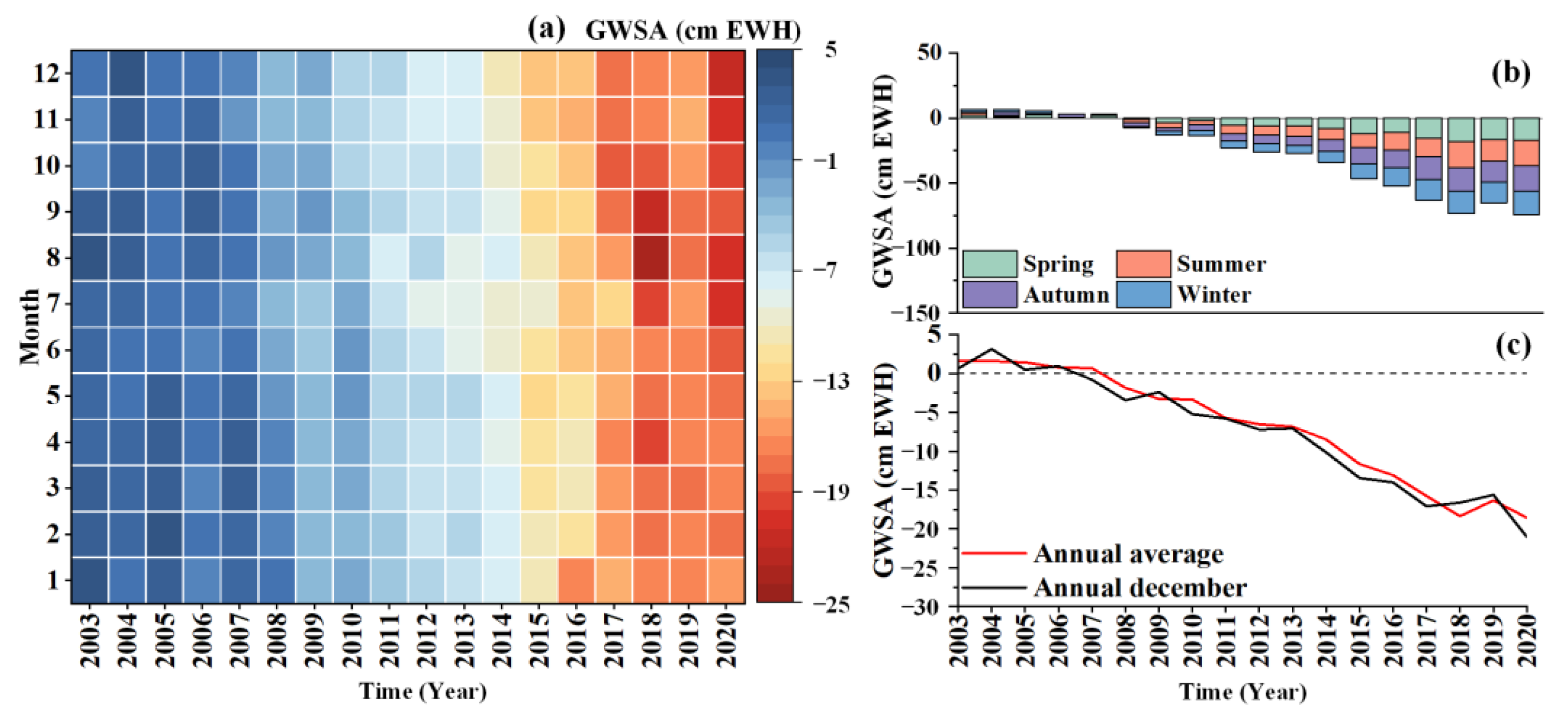
Between 2003 and 2007, groundwater storage in the study area remained relatively stable. However, groundwater storage has consistently decreased since 2008, especially in spring and summer, but increased seasonal rainfall has not led to a corresponding increase in groundwater storage. The decrease in groundwater storage gradually increased in the Piedmont plain, and it became even more severe from south to north.

(2)

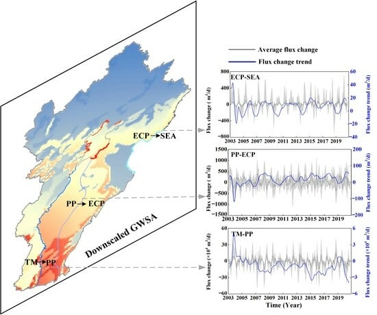
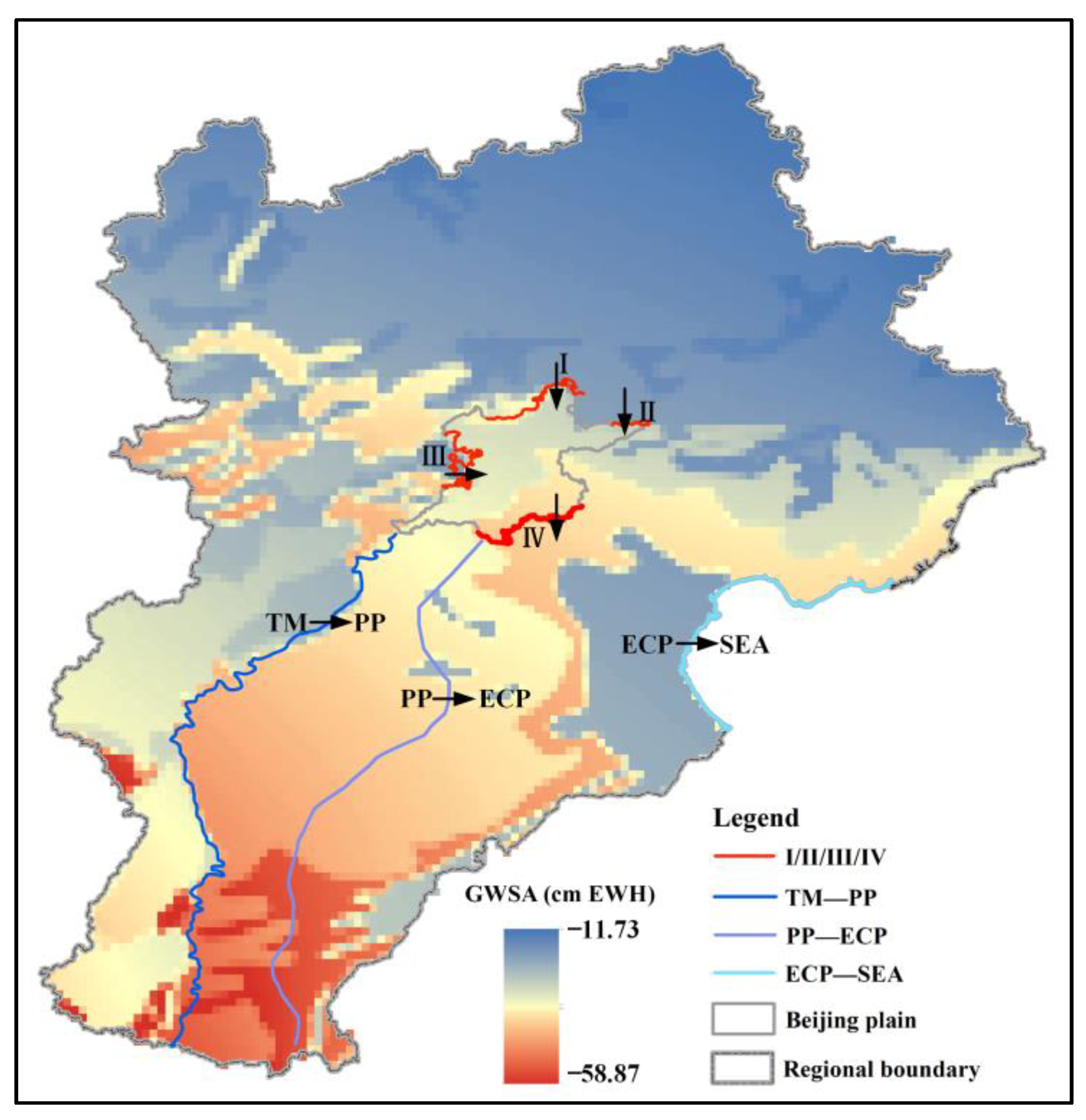
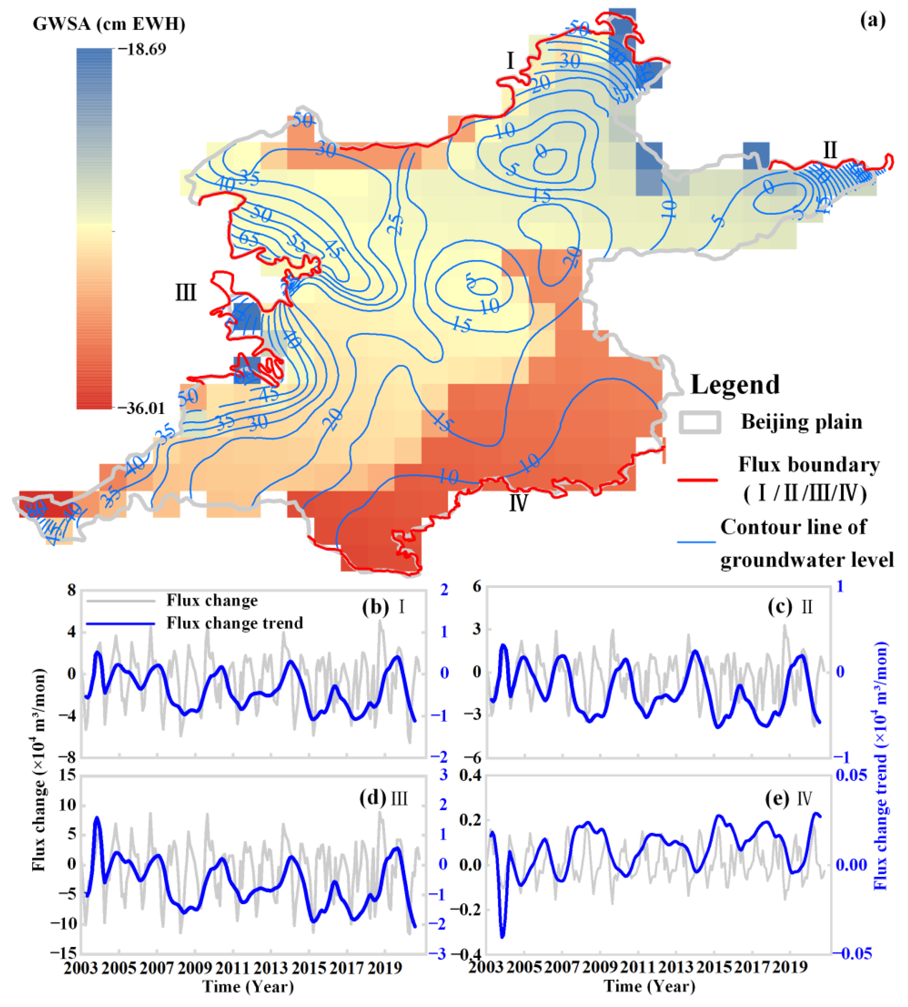
The groundwater exchange trends in the mountain front area calculated using 1° and 0.05° GWSA data were basically consistent. Naturally, the 0.05° GWSA data could better reflect the characteristics of groundwater exchange in small areas. Groundwater exchange exhibited a decreasing trend from the mountain area to the coastal areas. Groundwater exchange in the western Taihang Mountains was greater than that in the northern Yanshan Mountains and gradually decreased from south to north. From 2003 to 2007, groundwater exchange between the mountainous and plain areas decreased, and since 2008, it has shown an increasing trend. The change in groundwater exchange between the plain areas and coastal areas was relatively small, and the change trend was the opposite of that in the mountain plain area, which may be due to the lag in the lateral horizontal exchange between the mountain areas and plain areas and coastal areas.

(3)

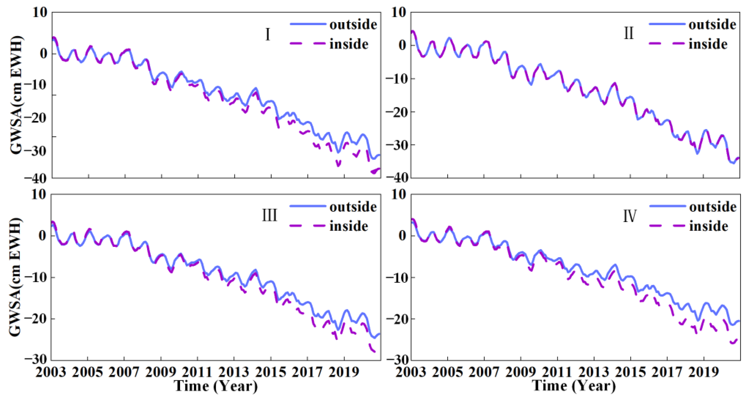
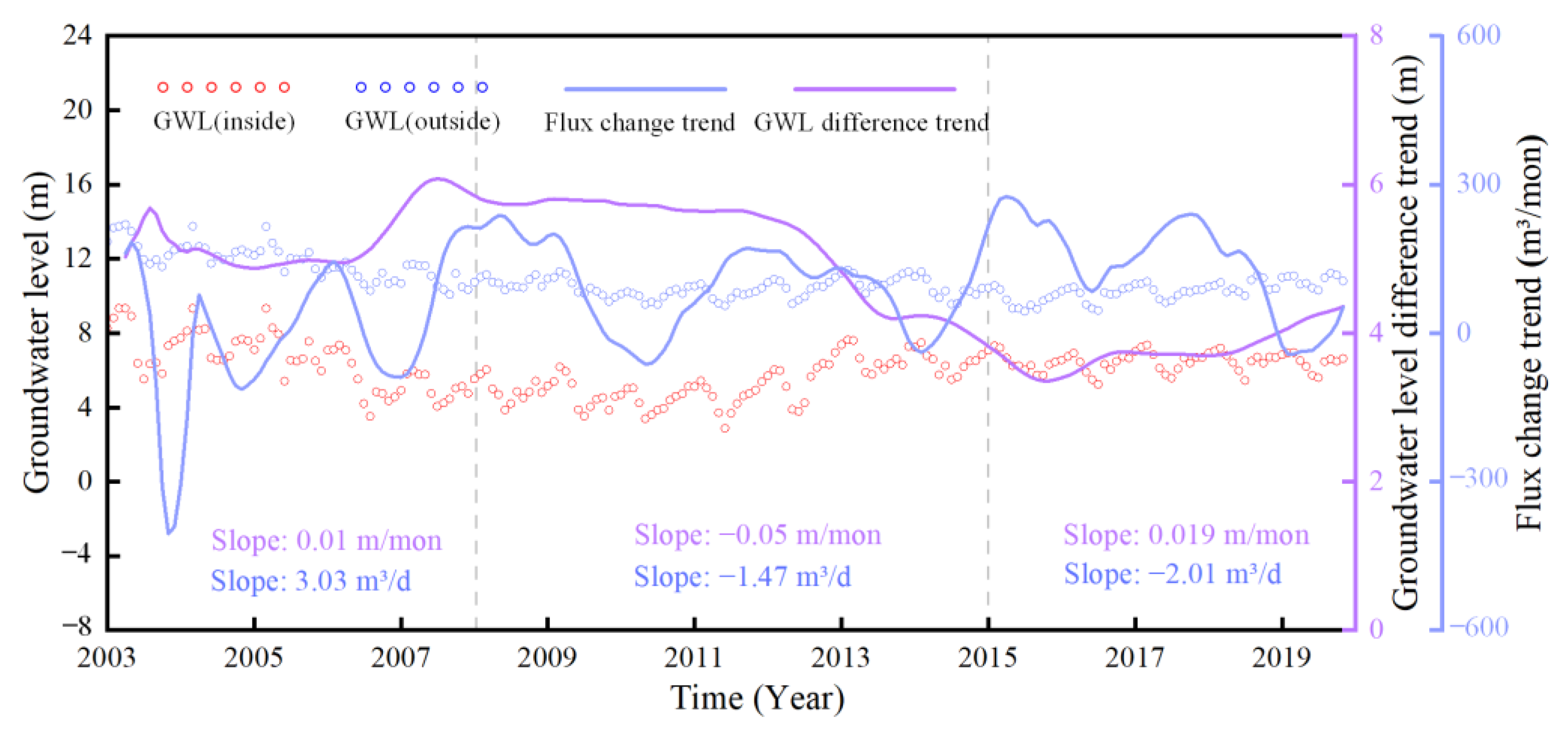
The change rate of groundwater exchange between the inner and outer boundaries and the change in the groundwater level difference were not always consistent. This may be attributed to the groundwater level in the monitoring wells being affected by local groundwater extraction or replenishment, resulting in a certain delay between the groundwater level and storage changes.

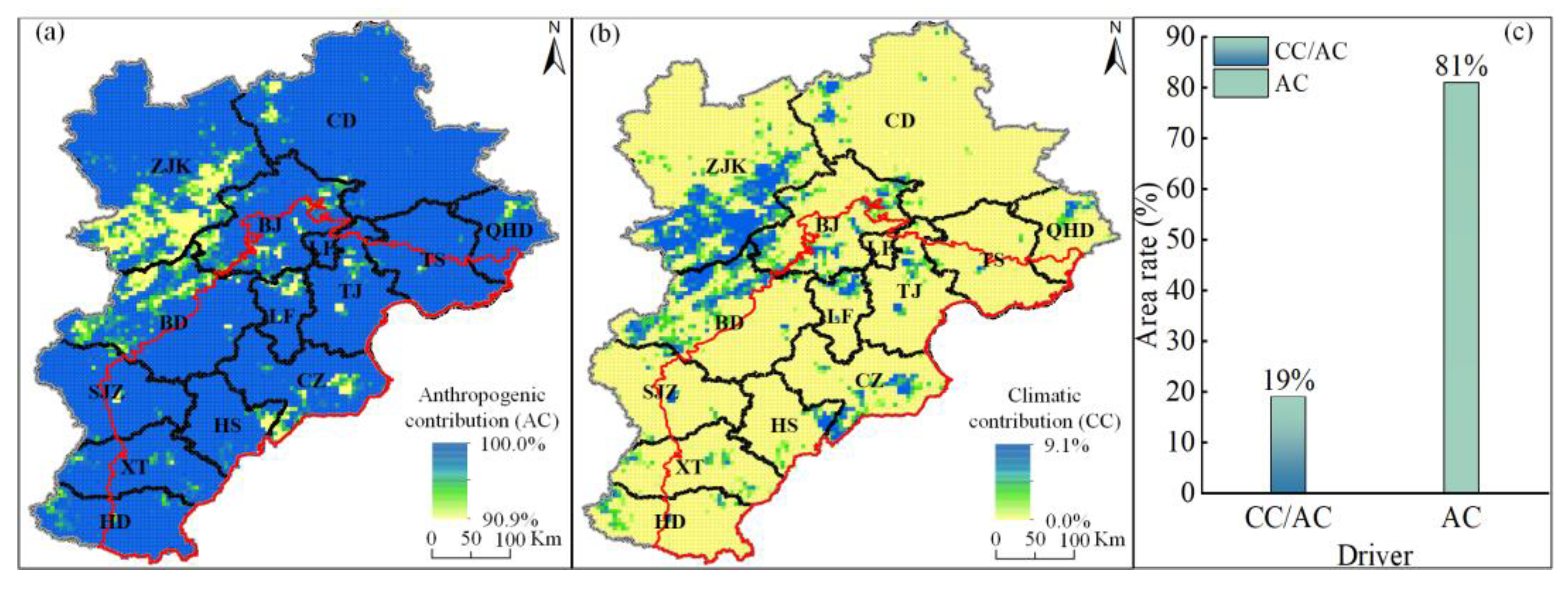
(4)

Anthropogenic activities accounted for more than 90.9% of the decrease in groundwater storage, with an average contribution of 98.2%. Climate factors played a secondary role, with contributions ranging from 0% to 9.1% and an average contribution rate of approximately 1.8%. Compared to human influences, climate change exhibited minimal independent control over groundwater storage variations.

References

- Herbert, C.; Döll, P. Global assessment of current and future groundwater stress with a focus on transboundary aquifers. Water Resour. Res. 2019, 55, 4760–4784. [Google Scholar] [CrossRef]
- Gleeson, T.; Cuthbert, M.; Ferguson, G.; Perrone, D. Global groundwater sustainability, resources, and systems in the Anthropocene. Annu. Rev. Earth Planet. Sci. 2020, 48, 431–463. [Google Scholar] [CrossRef]
- Gleeson, T.; VanderSteen, J.; Sophocleous, M.A.; Taniguchi, M.; Alley, W.M.; Allen, D.M.; Zhou, Y. Groundwater sustainability strategies. Nat. Geosci. 2010, 3, 378–379. [Google Scholar] [CrossRef]
- Rodell, M.; Famiglietti, J.S.; Wiese, D.N.; Reager, J.T.; Beaudoing, H.K.; Landerer, F.W.; Lo, M.-H. Emerging trends in global freshwater availability. Nature 2018, 557, 651–659. [Google Scholar] [CrossRef]
- Yeh, P.J.; Swenson, S.C.; Famiglietti, J.S.; Rodell, M. Remote sensing of groundwater storage changes in Illinois using the Gravity Recovery and Climate Experiment (GRACE). Water Resour. Res. 2006, 42, W12203. [Google Scholar] [CrossRef]
- Rodell, M.; Velicogna, I.; Famiglietti, J.S. Satellite-based estimates of groundwater depletion in India. Nature 2009, 460, 999–1002. [Google Scholar] [CrossRef]
- Famiglietti, J.S.; Lo, M.; Ho, S.L.; Bethune, J.; Anderson, K.J.; Syed, T.H.; Swenson, S.C.; de Linage, C.R.; Rodell, M. Satellites measure recent rates of groundwater depletion in California’s Central Valley. Geophys. Res. Lett. 2011, 38, L03403. [Google Scholar] [CrossRef]
- Longuevergne, L.; Scanlon, B.R.; Wilson, C.R. GRACE Hydrological estimates for small basins: Evaluating processing approaches on the High Plains Aquifer, USA. Water Resour. Res. 2010, 46, W11517. [Google Scholar] [CrossRef]
- Scanlon, B.R.; Longuevergne, L.; Long, D. Ground referencing GRACE satellite estimates of groundwater storage changes in the California Central Valley, USA. Water Resour. Res. 2012, 48, W04520. [Google Scholar] [CrossRef]
- Tran, H.; Zhang, J.; O’neill, M.M.; Ryken, A.; Condon, L.E.; Maxwell, R.M. A hydrological simulation dataset of the Upper Colorado River Basin from 1983 to 2019. Sci. Data 2022, 9, 16. [Google Scholar] [CrossRef]
- García-García, D.; Ummenhofer, C.C.; Zlotnicki, V. Australian water mass variations from GRACE data linked to Indo-Pacific climate variability. Remote Sens. Environ. 2011, 115, 2175–2183. [Google Scholar] [CrossRef]
- Forootan, E.; Awange, J.; Kusche, J.; Heck, B.; Eicker, A. Independent patterns of water mass anomalies over Australia from satellite data and models. Remote Sens. Environ. 2012, 124, 427–443. [Google Scholar] [CrossRef]
- Voss, K.A.; Famiglietti, J.S.; Lo, M.-H.; De Linage, C.; Rodell, M.; Swenson, S.C. Groundwater depletion in the Middle East from GRACE with implications for transboundary water management in the Tigris-Euphrates-Western Iran region. Water Resour. Res. 2013, 49, 904–914. [Google Scholar] [CrossRef]
- Feng, W.; Zhong, M.; Lemoine, J.; Biancale, R.; Hsu, H.; Xia, J. Evaluation of groundwater depletion in North China using the gravity recovery and climate experiment (GRACE) data and ground-based measurements. Water Resour. Res. 2013, 49, 2110–2118. [Google Scholar] [CrossRef]
- Huang, Z.; Pan, Y.; Gong, H.; Yeh, P.J.F.; Li, X.; Zhou, D.; Zhao, W. Subregional-scale groundwater depletion detected by GRACE for both shallow and deep aquifers in North China Plain. Geophys. Res. Lett. 2015, 42, 1791–1799. [Google Scholar] [CrossRef]
- Su, Y.; Guo, B.; Zhou, Z.; Zhong, Y.; Min, L. Spatio-temporal variations in groundwater revealed by GRACE and its driving factors in the Huang-Huai-Hai Plain, China. Sensors 2020, 20, 922. [Google Scholar] [CrossRef]
- Li, J.; Tang, H.; Rao, W.; Zhang, L.; Sun, W. Influence of South-to-North Water Transfer Project on the changes of terrestrial water storage in North China Plain. Chin. J. Univ. Chin. Acad. Sci. 2020, 37, 775–783. [Google Scholar] [CrossRef]
- Li, W.; Wang, L.; Yang, H.; Zheng, Y.; Cao, W.; Liu, K. The groundwater overexploitation status and countermeasure suggestions of the North China Plain. Chin. J. China Water Resour. 2020, 26–30. (In Chinese) [Google Scholar]
- Zhang, C.; Duan, Q.; Yeh, P.J.-F.; Pan, Y.; Gong, H.; Moradkhani, H.; Gong, W.; Lei, X.; Liao, W.; Xu, L.; et al. Sub-regional groundwater storage recovery in North China Plain after the South-to-North water diversion project. J. Hydrol. 2021, 597, 126156. [Google Scholar] [CrossRef]
- Zhang, H.; Zhang, L.L.; Li, J.; An, R.D.; Deng, Y. Monitoring the spatiotemporal terrestrial water storage changes in the Yarlung Zangbo River Basin by applying the P-LSA and EOF methods to GRACE data. Sci. Total. Environ. 2020, 713, 136274. [Google Scholar] [CrossRef]
- Zhang, J.; Liu, K.; Wang, M. Seasonal and interannual variations in China’s groundwater based on GRACE data and multisource hydrological models. Remote Sens. 2020, 12, 845. [Google Scholar] [CrossRef]
- Xu, Y.; Gong, H.; Chen, B.; Zhang, Q.; Li, Z. Long-term and seasonal variation in groundwater storage in the North China Plain based on GRACE. Int. J. Appl. Earth Obs. Geoinf. 2021, 104, 102560. [Google Scholar] [CrossRef]
- Ning, S.; Ishidaira, H.; Wang, J. Statistical downscaling of GRACE-derived terrestrial water storage using satellite and GLDAS products. J. Jpn. Soc. Civ. Eng. 2014, 70, 133–138. [Google Scholar] [CrossRef] [PubMed]
- Sun, A.Y. Predicting groundwater level changes using GRACE data. Water Resour. Res. 2013, 49, 5900–5912. [Google Scholar] [CrossRef]
- Seyoum, W.M.; Kwon, D.; Milewski, A.M. Downscaling GRACE TWSA Data into High-Resolution Groundwater Level Anomaly Using Machine Learning-Based Models in a Glacial Aquifer System. Remote Sens. 2019, 11, 824. [Google Scholar] [CrossRef]
- Zaitchik, B.F.; Rodell, M.; Reichle, R.H. Assimilation of GRACE terrestrial water storage data into a land surface model: Results for the Mississippi River Basin. J. Hydrometeorol. 2008, 9, 535–548. [Google Scholar] [CrossRef]
- Zhong, D.; Wang, S.; Li, J. Spatiotemporal downscaling of GRACE total water storage using land surface model outputs. Remote Sens. 2021, 13, 900. [Google Scholar] [CrossRef]
- Yin, W.; Hu, L.; Zhang, M.; Wang, J.; Han, S. Statistical downscaling of GRACE-derived groundwater storage using ET data in the North China Plain. J. Geophys. Res. Atmos. 2018, 123, 5973–5987. [Google Scholar] [CrossRef]
- Sun, J.; Hu, L.; Chen, F.; Sun, K.; Yu, L.; Liu, X. Downscaling simulation of groundwater storage in the Beijing, Tianjin, and Hebei regions of China based on GRACE data. Remote Sens. 2023, 15, 1490. [Google Scholar] [CrossRef]
- Cao, G.; Zheng, C.; Scanlon, B.R.; Liu, J.; Li, W. Use of flow modeling to assess sustainability of groundwater resources in the North China Plain. Water Resour. Res. 2013, 49, 159–175. [Google Scholar] [CrossRef]
- Ohmer, M.; Liesch, T.; Goeppert, N.; Goldscheider, N. On the optimal selection of interpolation methods for groundwater contouring: An example of propagation of uncertainty regarding inter-aquifer exchange. Adv. Water Resour. 2017, 109, 121–132. [Google Scholar] [CrossRef]
- Viaroli, S.; Mastrorillo, L.; Lotti, F.; Paolucci, V.; Mazza, R. The groundwater budget: A tool for preliminary estimation of the hydraulic connection between neighboring aquifers. J. Hydrol. 2018, 556, 72–86. [Google Scholar] [CrossRef]
- Cao, G.; Scanlon, B.R.; Han, D.; Zheng, C. Impacts of thickening unsaturated zone on groundwater recharge in the North China Plain. J. Hydrol. 2016, 537, 260–270. [Google Scholar] [CrossRef]
- Zhang, J.; Wang, X.; Hu, X.; Lu, H.; Gong, Y.; Wan, L. The Macro-characteristics of groundwater flow in the Badain Jaran Desert. J. Desert Res. 2015, 35, 774–782. (In Chinese) [Google Scholar] [CrossRef]
- Hu, L.; Xu, Z.; Huang, W. Development of a river-groundwater interaction model and its application to a catchment in Northwestern China. J. Hydrol. 2016, 543, 483–500. [Google Scholar] [CrossRef]
- Cook, P.G.; Lamontagne, S.; Berhane, D.; Clark, J.F. Quantifying groundwater discharge to Cockburn River, Southeastern Australia, using dissolved gas tracers 222Rn and SF6. Water Resour. Res. 2006, 42, W10411. [Google Scholar] [CrossRef]
- Li, F.; Song, X.; Tang, C.; Liu, C.; Yu, J.; Zhang, W. Tracing infiltration and recharge using stable isotope in Taihang Mt., North China. Environ. Geol. 2007, 53, 687–696. [Google Scholar] [CrossRef]
- Cook, P.G.; Rodellas, V.; Stieglitz, T.C. Quantifying surface water, porewater, and groundwater interactions using tracers: Tracer fluxes, water fluxes, and end-member concentrations. Water Resour. Res. 2018, 54, 2452–2465. [Google Scholar] [CrossRef]
- Manivannan, V.; Elango, L. Assessment of interaction between the aquifers by geochemical signatures in an urbanised coastal region of India. Environ. Earth Sci. 2021, 80, 218. [Google Scholar] [CrossRef]
- Chen, J.Y.; Tang, C.Y.; Shen, Y.J.; Sakura, Y.; Kondoh, A.; Shimada, J. Use of water balance calculation and tritium to examine the dropdown of groundwater table in the piedmont of the North China Plain (NCP). Environ. Geol. 2003, 44, 564–571. [Google Scholar] [CrossRef]
- Song, X.; Li, F.; Liu, C.; Tang, Q.; Zhang, W. Water cycle in Taihang Mountain and its recharge to groundwater in the North China Plain. J. Nat. Resour. 2007, 22, 398–408. (In Chinese) [Google Scholar]
- Pellicer-Martínez, F.; González-Soto, I.; Martínez-Paz, J.M. Analysis of incorporating groundwater exchanges in hydrological models. Hydrol. Process. 2015, 29, 4361–4366. [Google Scholar] [CrossRef]
- Yin, W.; Hu, L.; Zheng, W.; Jiao, J.J.; Han, S.; Zhang, M. Assessing underground water exchange between regions using GRACE data. J. Geophys. Res. Atmos. 2020, 125, e2020JD032570. [Google Scholar] [CrossRef]
- Guo, H.; Zhang, Z.; Cheng, G.; Li, W.; Li, T.; Jiao, J.J. Groundwater-derived land subsidence in the North China Plain. Environ. Earth Sci. 2015, 74, 1415–1427. [Google Scholar] [CrossRef]
- Gong, H.; Pan, Y.; Zheng, L.; Li, X.; Zhu, L.; Zhang, C.; Huang, Z.; Li, Z.; Wang, H.; Zhou, C. Long-term groundwater storage changes and land subsidence development in the North China Plain (1971–2015). Hydrogeol. J. 2018, 26, 1417–1427. [Google Scholar] [CrossRef]
- Li, X.; Ye, S.-Y.; Wei, A.-H.; Zhou, P.-P.; Wang, L.-H. Modelling the response of shallow groundwater levels to combined climate and water-diversion scenarios in Beijing-Tianjin-Hebei Plain, China. Hydrogeol. J. 2017, 25, 1733–1744. [Google Scholar] [CrossRef]
- Kendy, E.; Zhang, Y.; Liu, C.; Wang, J.; Steenhuis, T. Groundwater recharge from irrigated cropland in the North China Plain: Case study of Luancheng County, Hebei Province, 1949–2000. Hydrol. Process. 2004, 18, 2289–2302. [Google Scholar] [CrossRef]
- Zhao, Y.; Lu, C.; He, X.; Liu, R.; Liu, M.; Dong, L. Ten questions regarding groundwater overexploitation in North China—How can groundwater boost recovery of rivers and lakes. China Water 2023, 19–25. (In Chinese) [Google Scholar]
- Sun, Z.; Long, D.; Yang, W.; Li, X.; Pan, Y. Reconstruction of GRACE data on changes in total water storage over the global land surface and 60 basins. Water Resour. Res. 2020, 56, e2019WR026250. [Google Scholar] [CrossRef]
- Sun, J.; Hu, L.; Cao, X.; Liu, D.; Liu, X.; Sun, K. A dynamical downscaling method of groundwater storage changes using GRACE data. J. Hydrol. Reg. Stud. 2023, 50, 101558. [Google Scholar] [CrossRef]
- Scanlon, B.R.; Zhang, Z.; Save, H.; Wiese, D.N.; Landerer, F.W.; Long, D.; Longuevergne, L.; Chen, J. Global evaluation of new GRACE mascon products for hydrologic applications. Water Resour. Res. 2016, 52, 9412–9429. [Google Scholar] [CrossRef]
- Mo, S.; Zhong, Y.; Forootan, E.; Mehrnegar, N.; Yin, X.; Wu, J.; Feng, W.; Shi, X. Bayesian convolutional neural networks for predicting the terrestrial water storage anomalies during GRACE and GRACE-FO gap. J. Hydrol. 2022, 604, 127244. [Google Scholar] [CrossRef]
- Humphrey, V.; Gudmundsson, L. GRACE-REC: A reconstruction of climate-driven water storage changes over the last century. Earth Syst. Sci. Data 2019, 11, 1153–1170. [Google Scholar] [CrossRef]
- Deng, S.; Liu, S.; Mo, X.; Jiang, L.; Peter, G. Reconstruction dataset of spatial and temporal global terrestrial water storage anomalies (1981–2020). Digit. J. Glob. Chang. Data Repos. 2023, 2. [Google Scholar] [CrossRef]
- Li, F.; Kusche, J.; Chao, N.; Wang, Z.; Löcher, A. Long-term (1979-present) total water storage anomalies over the global land derived by reconstructing GRACE data. Geophys. Res. Lett. 2021, 48, e2021GL093492. [Google Scholar] [CrossRef]
- Cleveland, R.B.; Cleveland, W.S.; McRae, J.E.; Terpenning, I. STL: A seasonal trend decomposition procedure based on loess. J. Off. Stat. 1990, 6, 3–73. [Google Scholar]
- Sen, P.K. Estimates of the regression coefficient based on Kendall’s Tau. J. Am. Stat. Assoc. 1968, 63, 1379–1389. [Google Scholar] [CrossRef]
- Kendall, M.G. Rank Correlation Methods; Griffin: London, UK, 1975. [Google Scholar]
- Mann, H.B. Nonparametric tests against trend. Econometrica 1945, 13, 245–259. [Google Scholar] [CrossRef]
- Sun, Y.; Yang, Y.; Zhang, L.; Wang, Z. The relative roles of climate variations and human activities in vegetation change in North China. Phys. Chem. Earth Parts A/B/C 2015, 87, 67–78. [Google Scholar] [CrossRef]
- Pei, H.; Liu, M.; Jia, Y.; Zhang, H.; Li, Y.; Xiao, Y. The trend of vegetation greening and its drivers in the agro-pastoral ecotone of northern China, 2000–2020. Ecol. Indic. 2021, 129, 108004. [Google Scholar] [CrossRef]
- Liu, M.; Pei, H.; Shen, Y. Evaluating dynamics of GRACE groundwater and its drought potential in Taihang Mountain Region, China. J. Hydrol. 2022, 612, 128156. [Google Scholar] [CrossRef]
- Long, D.; Yang, W.; Scanlon, B.R.; Zhao, J.; Liu, D.; Burek, P.; Pan, Y.; You, L.; Wada, Y. South-to-North water diversion stabilizing Beijing’s groundwater levels. Nat. Commun. 2020, 11, 3665. [Google Scholar] [CrossRef]
- Yang, H.; Cao, W.; Zhi, C.; Li, Z.; Bao, X.; Ren, Y.; Liu, F.; Fan, C.; Wang, S.; Wang, Y. Evolution of groundwater level in the North China Plain in the past 40 years and suggestions on its overexploitation treatment. Geol. China 2021, 48, 1142–1155. (In Chinese) [Google Scholar]