Hierarchical Mixed-Precision Post-Training Quantization for SAR Ship Detection Networks

Abstract

Convolutional neural network (CNN)-based synthetic aperture radar (SAR) ship detection models operating directly on satellites can reduce transmission latency and improve real-time surveillance capabilities. However, limited satellite platform resources present a significant challenge. Post-training quantization (PTQ) provides an efficient method for pre-training neural networks to effectively reduce memory and computational resources without retraining. Despite this, PTQ faces the challenge of maintaining model accuracy, especially at low-bit quantization (e.g., 4-bit or 2-bit). To address this challenge, we propose a hierarchical mixed-precision post-training quantization (HMPTQ) method for SAR ship detection neural networks to reduce quantization error. This method encompasses a layerwise precision configuration based on reconstruction error and an intra-layer mixed-precision quantization strategy. Specifically, our approach initially utilizes the activation reconstruction error of each layer to gauge the sensitivity necessary for bit allocation, considering the interdependencies among layers, which effectively reduces the complexity of computational sensitivity and achieves more precise quantization allocation. Subsequently, to minimize the quantization error of the layers, an intra-layer mixed-precision quantization strategy based on probability density assigns a greater number of quantization bits to regions where the probability density is low for higher values. Our evaluation on the SSDD, HRSID, and LS-SSDD-v1.0 SAR Ship datasets, using different detection CNN models, shows that the YOLOV9c model with mixed-precision quantization at 4-bit and 2-bit for weights and activations achieves only a 0.28% accuracy loss on the SSDD dataset, while reducing the model size by approximately 80%. Compared to state-of-the-art methods, our approach maintains competitive accuracy, confirming the superior performance of the HMPTQ method over existing quantization techniques.

1. Introduction

Synthetic aperture radar (SAR) imagery has become an indispensable asset in Earth observation, offering unique capabilities that surpass the limitations of traditional optical imaging systems. By using microwave signals, SAR can penetrate cloud cover and operate at night, enabling continuous high-resolution imaging regardless of weather conditions. This versatility makes SAR invaluable for a wide range of applications, from environmental monitoring and disaster response to military surveillance and urban planning.

One of the most significant applications of SAR imagery is in target detection, where it plays a key role in identifying and classifying objects of interest. For instance, in the maritime domain, SAR imagery is used for ship detection [1,2,3], aiding in navigational safety, pirate detection, and maritime boundary monitoring. Additionally, SAR technology demonstrates unique value in water body detection [4,5], flood detection [6,7], and oil spill detection [8,9,10]. Water body detection contributes to water resource management and protection, flood detection enables the timely assessment of disaster risks and guides rescue operations, and oil spill detection is crucial for environmental protection and pollution control.

Traditional SAR image target detection methods, such as image segmentation [11] and Support Vector Machines (SVMs) [12], have been limited by the complexity of SAR imagery, including its unique signal properties and variable imaging conditions. The emergence of deep learning, particularly convolutional neural networks (CNNs), has revolutionized SAR image analysis by significantly improving accuracy and reliability through advanced feature extraction and pattern recognition. However, deploying these deep learning models on resource-constrained edge devices, like satellites, is challenging due to the high storage and transmission costs associated with large neural networks.

Quantization has recently emerged as an effective method for compressing neural networks, reducing storage size, and alleviating bandwidth pressure during parameter transmission [13,14,15]. The field of quantization technology can be divided into two main methods: quantization-aware training (QAT) [16,17,18] and post-training quantization (PTQ) [13,19,20,21,22,23,24,25,26,27,28]. Although QAT generally achieves better performance, it requires more computational resources and access to the full training dataset. PTQ, in contrast, allows for the quantization of pre-trained models using only a small calibration dataset or even without any dataset, addressing concerns over data privacy and enabling easier deployment on edge devices. Despite these advantages, achieving comparable performance to full precision models with low-bit quantization remains a major challenge for PTQ. This study aims to address this issue by proposing a more effective quantization strategy that maintains high accuracy while minimizing resource consumption.

Several layerwise mixed-precision PTQ techniques have been proposed to tackle this challenge [19,20,21,29]. Dong et al. [19] proposed Hessian-Aware Quantization (HAWQ), a layerwise quantization approach that uses the Hessian spectrum of a layer as an importance factor to select the quantization precision for each layer. However, this method requires the manual selection of quantization precision, which can be labor-intensive and time-consuming, particularly for large-scale models. To address the limitation, Dong et al. [20] proposed HAWQ-V2, which uses a Pareto frontier approach to automate mixed-precision allocation, achieving better accuracy than HAWQ. Nevertheless, the process of computing the Hessian matrix for each layer or basic module in HAWQ and HAWQ-V2 is computationally expensive, especially for deep neural networks like ResNet156 [30]. In addition, the memory demand for Hessian trajectory computation increases proportionally with the number of images as shown in Figure 1c. The number of images used to compute the Hessian trajectory can also affect model accuracy when using the same parameter constraints as illustrated in Figure 1d.

Figure 1. The YOLOV5n model, pre-trained on the SSDD dataset [31], is reduced in size by quantizing its weights and activations to 8/4-bit mixed precision and 8-bit precision, respectively. The subfigures illustrate the following: (a) weight quantization error sensitivity analysis with HAWQ-V2 [20], (b) weight quantization error sensitivity analysis with ZeroQ [21], (c) memory requirements for Hessian trace computation, and (d) Hessian trace computation under varying image conditions and the corresponding model accuracy under different parameter constraints.

To mitigate the impact of data requirements on the quantification process, Yaohui et al. [21] proposed ZeroQ, a novel zero-shot quantization framework to quantize pre-trained CNNs without relying on any training or validation data. This is achieved through the use of Kullback–Leibler (KL) divergence to evaluate sensitivity. However, while ZeroQ provides a data-free approach to quantization, it does not account for individual, layer-specific quantization errors. As a result, the quantization precision may be unevenly distributed across layers, potentially impacting the overall accuracy of the model (see Figure 1a,b).

Chauhan et al. [29] proposed a post-training mixed-precision quantization method based on first-order information, which evaluates layer sensitivity by computing the expected average norm of gradients near the convergence point. This method optimizes bit allocation through integer linear programming (ILP), reducing computational costs and the need for model retraining. However, it relies on gradient information, which requires calculating gradients during the backward pass, thus increasing computational complexity.

To address these challenges, this paper proposes a hierarchical mixed-precision post-training quantization (HMPTQ) method that aims to reduce quantization error while maintaining low computational cost and complexity. The overall process of HMPTQ is illustrated in Figure 2. The method first evaluates the layer sensitivity required for quantization based on the activation reconstruction error of each layer. Unlike previous methods, HMPTQ not only considers the error in a single layer but also accounts for dependencies between layers, which can impact the overall quantization accuracy. The HMPTQ strategy requires only a small portion of the validation dataset for forward inference and achieves a more accurate bit allocation with lower computational effort. Additionally, HMPTQ employs an intra-layer mixed-precision strategy that assigns different quantization bits to different regions within each layer, further reducing the quantization error. The experimental results demonstrate that the HMPTQ can effectively maintain model performance, which is of practical significance for resource-constrained deployment environments.

Figure 2. The overflow of our proposed hierarchical mixed-precision post-training quantization algorithm.

The remainder of this article is structured as follows: Section 2 provides an overview of related works, while Section 3 introduces the problem setting and the proposed HMPTQ method in detail. Section 4 presents a comprehensive account of the experimental setup and results analysis. Finally, Section 5 concludes the article.

2. Related Works

In this section, we provide a brief overview of the existing literature on the detection of SAR ships and the quantization of CNNs.

2.1. Synthetic Aperture Radar Ship Detection

Synthetic aperture radar satellites offer microwave remote sensing imagery that transcends the limitations of weather and light conditions, thus playing a vital role across various applications [1,2,3,4,5,6,7,8,9,10,32,33]. In recent years, the notable improvement in SAR image resolution has led to an escalating demand for the automatic interpretation and recognition of ship targets within these images. The introduction of deep learning technology has brought new breakthroughs in the recognition of ship targets in SAR images. Deep learning models, especially convolutional neural networks, have been widely applied in SAR image processing due to their powerful capabilities in feature extraction and image analysis.

Chen et al. [34] proposed an improved Faster R-CNN algorithm that successfully enhanced detection performance by replacing the backbone network, implementing online hard example mining, employing Soft-NMS algorithm, and adjusting the aspect ratios of anchors, achieving a 5% increase in mean average precision (mAP) on the HRSC2016 dataset. Furthermore, Chai et al. [35] significantly improved the detection accuracy for small targets, increasing the average precision (AP) from 0.79 to 0.89 on the satellite ship detection dataset (SSDD) dataset [31], by fusing multi-level features, introducing the convolutional block attention module (CBAM) to enhance feature extraction, and optimizing the region of interest (RoI) pooling algorithm to reduce quantization errors. The two-stage object detection algorithm is complex and time-consuming due to the need to set up numerous candidate regions in advance and correct them through the region proposal network (RPN). In contrast, the single-stage model omits the candidate region generation, directly performing detection to quickly provide results. The typical single-stage object detection algorithm is YOLO [36]. Wang et al. [37] enhanced YOLOV3 by optimizing the anchor box selection with K-means++ and employing focal loss, thereby improving the detection efficiency, accuracy, and model convergence. Liu et al. [38] mitigated the limitations of YOLOV5 by integrating GhostbottleNet, which uses dual GhostNet modules to refine the feature capture and reduce the generalized intersection over union (GIoU) metric, enhancing detection precision. Ge et al. [39] addressed the detection of small targets in SAR images by augmenting YOLOV7 with the channel attention mechanism and the bidirectional feature pyramid network. This approach enhances feature discernment and articulation, particularly for shallow features, and adjusts learning weights across scales. Evaluations on the rotated ship detection dataset in SAR images (RSDD-SAR) [40] revealed that the refined YOLOV7 algorithm substantially improves the detection and identification of small ship targets, achieving a 91.54% recognition accuracy, a 3.82% improvement over the original model. These research advancements demonstrate the positive role of deep learning in the field of maritime target detection, providing valuable insights for the further refinement of algorithms and their practical application.

Despite the remarkable achievements of CNN-based SAR ship detection methods, these models often have a large number of parameters and require substantial computational resources. This can be limiting in practical applications, especially when models need to be deployed on platforms with constrained resources.

2.2. Quantization

Neural network quantization reduces model size and computational requirements by converting floating-point numbers to integers, making it a key technique for effectively deploying deep learning models on resource-constrained devices while striving to maintain their performance. There are typically two main methods: quantization-aware training (QAT) and post-training quantization (PTQ).

QAT, as proposed by Google [16], incorporates pseudo-quantization nodes into the training process. During the forward pass, QAT employs quantized weights and activation outputs to process feature data, while the backward pass leverages floating-point 32-bit (FP32) weights for gradient computation, thereby training the network with the precision loss simulated by the non-quantized errors. Despite delivering robust performance, the demands of QAT for extensive time and data render it impractical in scenarios with constrained training resources or limited dataset availability.

PTQ provides a more efficient alternative to QAT, obviating the need for extensive datasets or retraining. It is distinguished by its simplicity, rapid deployment, and suitability for environments with data privacy constraints. Although PTQ is an efficient method that reduces the computational overhead compared to QAT, it may occasionally result in significant accuracy loss. The alternating optimization method, employed by EasyQuant [22], is utilized to address the issue of accuracy degradation by resolving the similarity between the quantization model and the original model output feature maps. Experiments show that EasyQuant can create a 7-bit network with almost the same accuracy as an 8-bit network.

Choukroun et al. [23] proposed a method to minimize the mean square error (MSE) for 4-bit uniform quantization. Experiments on ImageNet show that the INT4 linear quantization method decreases inference accuracy by only 3.00% top-1 and 1.70% top-5 compared to the FP32 model. Guan et al. [24] proposed 4-bit post-training quantization using row-wise uniform quantization with greedy search and non-uniform quantization using k-mean clustering. The 4-bit uniform quantization method using greedy search can reduce the model size to only 13.89% without affecting model quality.

Hubara et al. [26] developed a quantization method, adaptive quantization (AdaQuant), which can be used with different bit widths (16-bit, 8-bit, and 4-bit). By feeding calibration data into the network, AdaQuant is able to adjust the scaling factor in order to minimize MSE, thus maintaining the accuracy of the model. On the ImageNet dataset, 8-bit quantization of MobileNetV2 [41] only decreases top-1 accuracy by 0.50%. Qualcomm [14] introduced the adaptive round (AdaRound) method for PTQ to make quantization algorithms more adaptable. This approach differs from traditional rounding techniques by deciding whether to round floating-point values to the nearest integer on the right or left during weight quantization. A second-order Taylor expansion shows that standard rounding is not the best. AdaRound achieves 4-bit quantization of ResNet18 and ResNet50 [30] with only a 1.00% loss in accuracy, eliminating the need for network fine-tuning.

Jun et al. [13] proposed the piecewise linear quantization (PWLQ) method to improve the precision of quantized models. PWLQ divides the range into three parts: the center and two sides of the weight distribution. Each segment obtains the same number of points. This method improves precision in the central region, which improves the accuracy of the quantized model.

Yuhang et al. [27] introduced block reconstruction quantization (BRECQ), an innovative PTQ framework that addresses second-order errors during the quantization process through block reconstruction. This approach balances cross-layer dependencies and generalization error by utilizing the Gauss–Newton matrix to analyze and optimize these errors. For the first time, BRECQ pushes the limits of PTQ down to 2-bit weight quantization without significant accuracy loss, enabling the rapid generation of quantized models. Furthermore, BRECQ incorporates mixed-precision techniques to enhance the performance of quantized models by approximating sensitivities both between and within layers. Xiuying et al. [28] introduced a randomly dropping quantization (QDrop), a groundbreaking method for extremely low-bit PTQ. This approach enhances model accuracy by randomly omitting the quantization of activation functions and leveraging the concept of flatness in calibration and test data to optimize low-bit models. QDrop has significantly boosted PTQ performance across diverse tasks, such as computer vision and natural language processing, setting a new standard with accuracy improvements of up to 51.49% for 2-bit activation quantization. Despite these advances, there is still room for improvement in how well quantized models work in different situations.

3. Methods

3.1. Problem Setting

Given a pre-trained CNN f with L layers and ${\left\{{\mathbf{W}}^l\right\}}_{l=1}^L$, where ${\mathbf{W}}^l$ is the weight parameter tensor of the l-th layer, a typical CNN often consists of linear convolutional computation and non-linear activation computation as follows:

$${\mathbf{Z}}^l={\mathbf{W}}^l·{\mathbf{X}}^{l-1}+{\mathbf{b}}^l,$$

(1)

$${\mathbf{X}}^l=\varphi \left({\mathbf{Z}}^l\right),$$

(2)

where $\varphi (·)$ is the activation function. ${\mathbf{X}}^{l-1}$ denotes the input of the l-th layer. ${\mathbf{b}}^l$ denotes the bias of the l-th convolutional layer.

For network weight quantization, we aim to find the low-bit weight tensors $\widehat{\mathbf{W}}$ that can minimize the quantization loss [14] as follows:

$$arg\underset{\Delta \mathbf{W}}{min}E(\mathcal{L}(\mathbf{W}+\Delta \mathbf{W},\mathbf{X})-\mathcal{L}(\mathbf{W},\mathbf{X})),$$

(3)

where $\mathcal{L}$ is the loss function. $\Delta \mathbf{W}$ represents quantization error. We leverage Taylor expansion to analyze the target, which reveals the quantization interactions among weights:

$$\begin{array}{cc}\hfill & \mathcal{L}(\mathbf{W}+\Delta \mathbf{W},\mathbf{X})-\mathcal{L}(\mathbf{W},\mathbf{X})\hfill \\ \hfill & =\Delta {\mathbf{W}}^T·{\nabla }_{\mathbf{W}}\mathcal{L}(\mathbf{W},\mathbf{X})\hfill \\ \hfill & +{\displaystyle \frac{1}{2}}\Delta {\mathbf{W}}^T·{\nabla }_{\mathbf{W}}^2\mathcal{L}(\mathbf{W},\mathbf{X})·\Delta \mathbf{W}\hfill \\ \hfill & +\mathcal{O}(\Delta \mathbf{W}),\hfill \end{array}$$

(4)

After the pre-trained model has successfully converged, the first term (${\nabla }_{\mathbf{W}}\mathcal{L}(\mathbf{W},\mathbf{X})\approx 0$) and $\mathcal{O}(\Delta \mathbf{W})$ can be neglected. According to Equation (4), to minimize the weight quantization loss, our objective is therefore to solve

$$arg\underset{\Delta \mathbf{W}}{min}\Delta {\mathbf{W}}^T·{\nabla }_{\mathbf{W}}^2\mathcal{L}(\mathbf{W},\mathbf{X})·\Delta \mathbf{W},$$

(5)

Assuming that there is no inter-layer dependency, we can relax Equation (5) to the per-layer optimization problem, namely,

$$arg\underset{\Delta {\mathbf{W}}^l}{min}\Delta {{\mathbf{W}}^l}^T·{\nabla }_{{\mathbf{W}}^l}^2\mathcal{L}({\mathbf{W}}^l,{\mathbf{X}}^l)·\Delta {\mathbf{W}}^l,$$

(6)

The second-order derivatives ${\nabla }_{{\mathbf{W}}^l}^2\mathcal{L}({\mathbf{W}}^l,{\mathbf{X}}^l)$ are the Hessian matrix with respect to ${\mathbf{W}}^l$ and are defined as

$$\begin{array}{c}\hfill {\nabla }_{{\mathbf{W}}^l}^2\mathcal{L}({\mathbf{W}}^l,{\mathbf{X}}^l)={\displaystyle \frac{{\partial }^2\mathcal{L}({\mathbf{W}}^l,{\mathbf{X}}^l)}{\partial {\left({\mathbf{W}}^l\right)}^2}}\\ \hfill ={\displaystyle \frac{\partial }{\partial {\mathbf{W}}^l}}\left[{\displaystyle \frac{\partial \mathcal{L}({\mathbf{W}}^l,{\mathbf{X}}^l)}{\partial {\mathbf{Z}}^l}}\right]·{\displaystyle \frac{\partial {\mathbf{Z}}^l}{\partial {\mathbf{W}}^l}}\\ \hfill ={\displaystyle \frac{{\partial }^2\mathcal{L}({\mathbf{W}}^l,{\mathbf{X}}^l)}{\partial {\left({\mathbf{Z}}^l\right)}^2}}·{\mathbf{X}}^{l-1}·{{\mathbf{X}}^{l-1}}^T,\end{array}$$

(7)

By substituting Equation (6) into Equation (7), we obtain the approximate error caused by the weight quantization as follows:

$$\begin{array}{c}\hfill E\left({\widehat{\mathbf{W}}}^l\right)=\Delta {{\mathbf{W}}^l}^T·{\nabla }_{{\mathbf{W}}^l}^2\mathcal{L}({\mathbf{W}}^l,{\mathbf{X}}^l)·\Delta {\mathbf{W}}^l\\ \hfill \approx {\displaystyle \frac{{\partial }^2\mathcal{L}({\mathbf{W}}^l,{\mathbf{X}}^l)}{\partial {\left({\mathbf{Z}}^l\right)}^2}}·{({\mathbf{Z}}^l-{\widehat{\mathbf{W}}}^{\mathbf{l}}{\mathbf{X}}^{l-1})}^2,\end{array}$$

(8)

The weighted average minimization problem, as mentioned, involves optimizing a weighted average of the activation quantization error with a weight coefficient ${\displaystyle \frac{{\partial }^2\mathcal{L}({\mathbf{W}}^l,{\mathbf{X}}^l)}{\partial {\left({\mathbf{Z}}^l\right)}^2}}$. However, this problem is challenging to optimize due to the involvement of second-order derivatives, which can only be obtained through back-propagation. To address this issue, we relax the weighted average minimization problem into an unweighted average minimization problem as follows:

$$\underset{{\widehat{\mathbf{W}}}^{\mathbf{l}}}{arg\; min}\left|\right|{\mathbf{Z}}^l-{\widehat{\mathbf{W}}}^{\mathbf{l}}{\mathbf{X}}^{l-1}{\left|\right|}_F^2,$$

(9)

In the optimization process described above, researchers refined the weights to optimize the model and avoided calculating the Hessian matrix. However, the inter-layer dependencies were not considered in Equation (9). Therefore, in this paper, we propose using the minimum reconstruction error of each layer and the loss error of adjacent layer quantization to build the quantization sensitivity for each layer. Then, an integer linear programming (ILP) algorithm is utilized to search for the quantization precision bits for each layer. Following this, the probability density-based quantization method is adopted for channel-wise quantization to reduce the quantization error for each layer.

3.2. Reconstruction Error-Based Precision Configuration

Given the analysis, the quantization error $\mathsf{\Omega }$ for a pre-trained model f with L layers is expressed as

$$\mathsf{\Omega }\left(f\right)=\sum _{l=1}^L{\mathsf{\Omega }}^l=\sum _{l=1}^L({\mathsf{\Omega }}_r^l+{\lambda }_l·{\mathsf{\Omega }}_{loss}^l),$$

(10)

where ${\mathsf{\Omega }}_r^l$ represents the reconstruction error for layer l, and ${\mathsf{\Omega }}_{loss}^l$ captures the loss error caused by quantization:

$${\mathsf{\Omega }}_r^l={∥Q\left({\mathbf{W}}^l\right){\mathbf{X}}^{l-1}-{\mathbf{W}}^l{\mathbf{X}}^{l-1}∥}_2^2,$$

(11)

$${\mathsf{\Omega }}_{loss}^l=\mathcal{L}({\widehat{\mathbf{W}}}_{l-1},{\widehat{\mathbf{W}}}_l)-max(\mathcal{L}\left({\widehat{\mathbf{W}}}_{l-1}\right),\mathcal{L}\left({\widehat{\mathbf{W}}}_l\right)),$$

(12)

The weighting factor ${\lambda }_l$ balances these two components:

$${\lambda }_l={\displaystyle \frac{E\left({\mathsf{\Omega }}_r^l\right)}{E\left({\mathsf{\Omega }}_{loss}^l\right)}},$$

(13)

To allocate the quantization bits efficiently for weights across different layers while adhering to parameter constrains, we solve the following optimization problem:

$$\begin{array}{c}\hfill arg\underset{{\left\{b_l\right\}}_{l=1}^L}{min}\sum _{l=1}^L{\mathsf{\Omega }}^l\left(b_l\right),\\ \hfill s.t.\sum _{l=1}^L{P}_l\left(b_l\right)\le P_{limit},\end{array}$$

(14)

where $b_l$ represents the bit allocation for layer l, $P_l$ denotes the parameter count for layer l as a function of its bit allocation, and $P_{limit}$ is the pre-defined parameter limit on the total parameter count. This framework optimizes bit allocation to balance precision and resource constraints effectively.

3.3. Intra-Layer Mixed-Precision Quantization

In neural network quantization, substantial errors may arise from clipping outlier values beyond the quantization range. Although such outliers are rare, they significantly influence the precision of the quantized model. Our methodology addresses this issue by selectively assigning higher bit widths to influential, albeit atypical, high-value outliers, thereby mitigating the degradation of the precision inherent in quantization.

The standard histogram, widely used to illustrate data distribution, hinges on the critical selection of bin size, which can significantly alter the resulting visualization as depicted in Figure 3a. Despite variations in visualization, the underlying probability distribution of the data remains unaffected as shown in Figure 3b and Figure 4b. To refine the analysis, this study introduces kernel density estimation (KDE) to assess the probability density of weights within pre-trained neural networks. KDE offers a superior, continuous estimation of the weight distribution, enabling the identification of diverse value ranges and the implementation of a dynamic quantization scheme with variable bit widths. This approach adeptly minimizes quantization errors across the spectrum of weight values, including the rare but significant outliers, thus enhancing the fidelity of the quantized model.

Figure 3. The pre-trained YOLOV5n model’s weight distribution on the SSDD dataset is as follows: (a) illustrates the histogram statistics and the corresponding fitted probability distribution curves under various bins conditions for the third convolutional layer; (b) displays the probability distribution of the weights in the third convolutional layer, alongside the quantization ranges defined by different probability thresholds.

Figure 4. The distribution of activations in the pre-trained YOLOV5n model on the SSDD dataset is characterized as follows: (a) presents the activation histograms of the calibration dataset, specifically focusing on the sixth and tenth SiLU layers; (b) illustrates the probability distribution of activations in the tenth SiLU layer, including the quantization intervals delineated by varying probability thresholds.

Let $\mathbf{R}=\{r_1,r_2,\dots ,r_N\}$ denote a set of real-valued parameters in a neural network. We define their probability density function as $\mathcal{D}$. Utilizing the Gaussian kernel function for its desirable properties of smoothness and differentiability, we perform KDE as follows:

$$\mathcal{D}\left(r\right)={\displaystyle \frac{1}{N}}\sum _{i=1}^N{\displaystyle \frac{1}{\sqrt{2\pi h^2}}}·e^{-{\displaystyle \frac{{(r-r_i)}^2}{2h^2}}},$$

(15)

$$h={\left({\displaystyle \frac{4{\sigma }^5}{3N}}\right)}^{1/5},$$

(16)

where h represents the bandwidth parameter, pivotal for KDE resolution. The bandwidth is determined using Silverman’s rule, a standard method for balancing the trade-off between overfitting and underfitting. $\sigma$ is the standard deviation of the dataset $\mathbf{R}$, and N is the total number of parameters. This approach ensures a robust estimation applicable to both weights and activations, providing a versatile framework for quantization in neural networks.

To minimize the quantization error, we implement piecewise quantization for each layer. Identifying segmentation points is a fundamental and critical step in this process. This paper focuses on piecewise quantization employing 2-bit, 4-bit and 8-bit precisions. For weight quantization in neural networks, we exploit the symmetric nature of weight distributions to identify key percentiles ${\beta }_2$ and ${\beta }_1$ as shown in Figure 3b, complementing our set of breakpoints. These breakpoints meticulously segment the quantization range of weights, defined from $mi{n}_{w\_val}$ to $ma{x}_{w\_val}$, into three intervals: $R_1$ = [$-{\beta }_1$, ${\beta }_1$] as the central region around zero, earmarked for 2-bit quantization, $R_2$ = [$-{\beta }_2$, $-{\beta }_1$) ∪ (${\beta }_1$, ${\beta }_2$] as the intermediate region, allocated for 4-bit quantization, and $R_3$ = [$mi{n}_{w\_val}$, $-{\beta }_2$) ∪ (${\beta }_2$, $ma{x}_{w\_val}$] as the outer bounds, reserved for 8-bit quantization. For activation quantization, given their often asymmetric distribution, we apply a streamlined approach using only two breakpoints ${\beta }_1$ and ${\beta }_2$ to divide the activation range from $mi{n}_{a\_val}$ to $ma{x}_{a\_val}$ into three regions: $R_1$ = [$mi{n}_{a\_val}$, ${\beta }_1$], $R_2$ = (${\beta }_1$, ${\beta }_2$), and $R_3$ = [${\beta }_2$, $ma{x}_{a\_val}$].

During quantization, we define three probability-based partition regions, $R_1$, $R_2$, and $R_3$, with each region being quantized with precisions of 2-bit, 4-bit, and 8-bit, and their respective probabilities denoted as $p_1$, $p_2$, and $p_3$. These probabilities are closely related to the number of quantization bits allocated to the current layer. For example, if a layer is allocated 4-bit for quantization, the probability $p_2$ should be within the 70% ∼ 90% range. The sum of the probabilities of all partition region must equal 1, satisfying the condition $p_1+p_2+p_3=1$, and each partition region’s probability must be strictly greater than 0, that is, $p_1>0$ and $p_3>0$.

To enhance hardware compatibility and streamline implementation, our proposed piecewise quantization strategy utilizes the uniform affine quantization method. Given a real-valued input r, the uniform affine quantization can be defined as follows:

$$r_{int}=clip(round\left({\displaystyle \frac{r}{s}}\right)+z),$$

(17)

$$\widehat{r}=s(r_{int}-z),$$

(18)

$$Q\left(r\right)=\widehat{r},$$

(19)

where s is the step size, and z is the zero-point. The uniform affine quantization function $Q\left(r\right)$ can then be applied to each interval $R_i$ with the corresponding $z_i$ and $s_i$ to yield the quantized value

$$Q\left(r\right)=\left\{\begin{array}{cc}{s}_1(clip(round\left({\displaystyle \frac{r}{s_1}}\right)+z_1)-z_1)\hfill & \mathrm{if}r\in R_1,\hfill \\ s_2(clip(round\left({\displaystyle \frac{r}{s_2}}\right)+z_2)-z_2)\hfill & \mathrm{if}r\in R_2,\hfill \\ s_3(clip(round\left({\displaystyle \frac{r}{s_3}}\right)+z_3)-z_3)\hfill & \mathrm{if}r\in R_3.\hfill \end{array}\right.$$

(20)

Assuming a layer in a neural network is assigned k-bit quantization precision, resulting in quantization error denoted as $E\left(k\right)$, when employing piecewise quantization for this layer, the error is partitioned into three components corresponding to the different regions $R_1$, $R_2$, and $R_3$, represented as E($R_1$, 2), E($R_2$, 4), and E($R_3$, 8). The conditions that the quantization breakpoints must satisfy are as follows:

$$\begin{array}{cc}\hfill & arg\underset{p_1,p_2,p_3}{min}(E(R_1,2)+E(R_2,4)+E(R_3,8)),\hfill \\ \hfill & \mathrm{s}.\mathrm{t}.E(R_1,2)+E(R_2,4)+E(R_3,8)<E\left(k\right),\hfill \\ \hfill & p_1+p_2+p_3=1,\hfill \\ \hfill & p\left(k\right)\in [0.7,0.9],k\in \{2,4,8\}.\hfill \end{array}$$

(21)

The goal of this constraint is to achieve a total quantization error that is less than half of what would be expected from a uniform k-bit quantization across the entire range of values. This refined quantization strategy aims to allocate higher precision to the regions of the distribution that contain a substantial portion of the data, thus improving the overall accuracy of the quantized model while still respecting the bit allocation constraints.

4. Experiment and Results

In this section, we evaluate the performance of our proposed method. All experiments are conducted using PyTorch 1.10.0, Python 3.8 and Torchvision 0.13.0, with CUDA 11.3 support. The hardware setup consists of a single NVIDIA GeForce RTX 3090 GPU with 24 GB memory and an Intel Xeon(R) Silver 4215R CPU@ 3.20 GHz.

4.1. Dataset Description

The proposed method is assessed using three SAR ship detection datasets: SSDD [31], HRSID [42], and LS-SSDD-v1.0 [43]. The SSDD dataset comprises 1160 SAR images (ranging from 1 m to 15 m resolution) sourced from RadarSat-2, TerraSAR-X, and Sentinel-1 sensors. The HRSID dataset consists of 5604 SAR images (ranging from 0.5 m to 3 m resolution) from Sentinel-1, TerraSAR-X, and TanDEM sensors. The LS-SSDD-v1.0 dataset includes 9000 SAR images (at 5 m and 20 m resolutions) from Sentinel-1 SAR. To ensure uniformity, all datasets are resized to 640 × 640 pixels. The training set to test set ratios are approximately 8:2 for SSDD, 6.5:3.5 for HRSID, and 2:1 for LS-SSDD-v1.0. Examples of these datasets can be seen in Figure 5.

Figure 5. Examples from the SSDD, HRSID, and LS-SSDD-v1.0 datasets are illustrated. The green box denotes the labeled ground truth box.

4.2. Experimental Setting

In order to validate the effectiveness of our proposed method, we initially established a performance benchmark for the YOLOV5n [44] and YOLOV9c [45] models. This was accomplished by employing the official training parameters on the SSDD, HRSID, and LS-SSDD datasets, thereby ensuring a robust and standardized foundation for our comparative analysis. YOLOV5n was trained with a batch size of 32, a learning rate of 0.00334, and the stochastic gradient descent (SGD) optimizer, using a momentum of 0.74832 and a weight decay of 0.00025. The training lasted for 300 epochs with 640 × 640 input images and an IoU threshold of 0.5 to ensure optimal performance and robustness. Meanwhile, YOLOV9c was trained with a batch size of 16, a learning rate of 0.01, and the SGD optimizer, with a momentum of 0.937 and a weight decay of 0.0005. The training ran for 300 epochs using 640 × 640 input images, with an IoU threshold of 0.5 to achieve similar goals.

During mixed-precision allocation, $P_{limit}$ is set to half of the original parameters, and reconstruction error is computed with a validation set of 32, optimizing efficiency while maintaining accuracy.

In our study, ‘W84’ denotes weight quantization with a layerwise mixed-precision distribution of 8-bit and 4-bit, where each layer uses a single quantization bit. Conversely, ‘WP84’ signifies weight quantization with a layerwise mixed-precision distribution of 8-bit and 4-bit, where each layer employs piecewise mixed-precision quantization with a precision set of {8, 4, 2}. Similarly, ‘A84’ represents activation quantization with a layerwise mixed-precision distribution of 8-bit and 4-bit, using a single quantization bit per layer. ‘AP84’ indicates activation quantization with a layerwise mixed-precision distribution of 8-bit and 4-bit, where each layer uses piecewise mixed-precision quantization with a precision set of {8, 4, 2}.

To accurately evaluate the performance of different methods, we adopt several evaluation metrics, including parameters (Params) and mean average precision (mAP).

4.3. Performance Evaluation

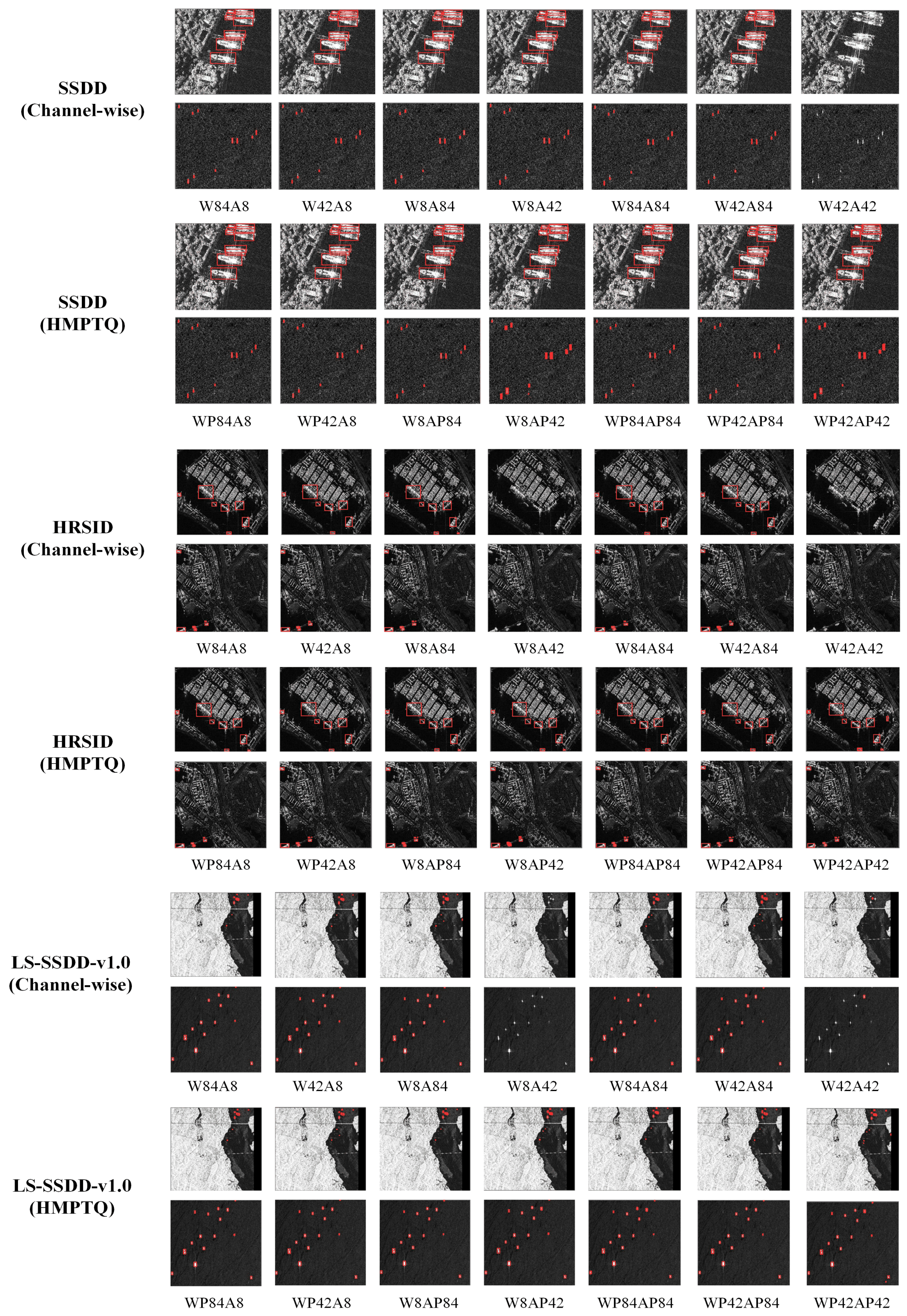
4.3.1. Experiments on Different Quantization Methods

To evaluate our proposed intra-layer mixed-precision quantization method, we conducted experiments using our proposed reconstruction error-based layerwise mixed-precision configuration method for bit configuration in each layer. Each layer’s quantization strategy was implemented in a channel-wise manner and compared against the channel-wise uniform affine quantization method, denoted as ’Channel-wise’. Furthermore, to provide additional insight into the effection of the proposed intra-layer mixed-precision quantization method, we implemented three state-of-the-art quantization methods: PWLQ [13], AdaRound [14], and Bit-Shrinking [15]. These techniques were included in the comparative analysis to benchmark the performance of our proposed method.

(1) Results

For the YOLOV5n model, as illustrated in Table 1, the FP32 baseline achieved high mAP scores of 98.21%, 92.21%, and 75.48% on the SSDD, HRSID, and LS-SSDD-v1.0 datasets, respectively. After applying channel-wise quantization, particularly with the W84A8 configuration, there was a slight mAP drop. For example, on the SSDD dataset, the mAP decreased by 0.03% to 98.18%. However, this method significantly reduced parameters by 77.30%. The WP84A8 method improved mAP slightly, achieving 98.27%, with a 77.04% parameter reduction. The WP42A8 method achieved the best result on SSDD, with a 98.38% mAP and an 84.01% reduction in parameters.

Table 1. Comparison results of our proposed intra-layer mixed-precision quantization and the channel-wise uniform affine quantization for YOLOV5n and YOLOV9c on SSDD, HRSID, and LS-SSDD-v1.0 datasets. The symbol ↓ indicates a decrease.

YOLOV5n
		SSDD				HRSID				LS-SSDD-v1.0
Method	Bits	Params	mAP	Params↓	$\Delta$mAP	Params	mAP	Params↓	$\Delta$mAP	Params	mAP	Params↓	$\Delta$mAP
	(W/A)	(MB)	(%)	(%)	(%)	(MB)	(%)	(%)	(%)	(MB)	(%)	(%)	(%)
Baseline	FP32	7.04	98.21	-	-	7.04	92.21	-	-	7.04	75.48	-	-
Channel-wise	W84A8	1.60	98.18	77.30	−0.03	1.60	92.25	77.33	0.04	1.56	72.70	77.86	−2.78
Channel-wise	W42A8	0.97	97.47	86.23	−0.74	0.97	92.18	86.29	−0.03	0.95	72.36	86.47	−3.12
Channel-wise	W8A84	2.02	97.67	71.33	−0.54	2.02	91.85	71.33	−0.36	2.02	73.22	71.33	−2.26
Channel-wise	W8A42	2.02	16.65	71.33	−81.56	2.02	21.04	71.33	−71.17	2.02	31.93	71.3	−43.55
Channel-wise	W84A84	1.56	97.62	77.83	−0.59	1.60	91.97	77.30	−0.24	1.56	73.56	77.88	−1.92
Channel-wise	W42A84	0.96	97.32	86.38	−0.89	0.97	92.04	86.26	−0.17	0.95	72.48	86.47	−3.00
Channel-wise	W42A42	0.94	11.48	86.64	−86.73	0.97	25.38	86.24	−66.83	0.95	30.54	86.47	−44.94
HMPTQ	WP84A8	1.62	98.27	77.04	0.06	1.67	92.19	76.28	−0.02	1.67	73.39	76.26	−2.09
HMPTQ	WP42A8	1.13	98.38	84.01	0.17	1.14	92.07	83.80	−0.14	1.14	73.53	83.88	−1.93
HMPTQ	W8AP84	2.02	98.09	71.33	−0.12	2.02	92.16	71.33	−0.05	2.02	73.77	71.33	−2.71
HMPTQ	W8AP42	2.02	96.89	71.33	−1.32	2.02	89.30	71.33	−1.91	2.02	70.17	71.33	−5.31
HMPTQ	WP84AP84	1.64	97.90	76.70	−0.31	1.67	92.12	76.33	−0.09	1.65	72.63	76.63	−2.85
HMPTQ	WP42AP84	1.11	98.18	84.21	−0.03	1.14	92.14	83.74	−0.07	1.14	72.80	83.88	−2.68
HMPTQ	WP42AP42	1.11	96.86	84.21	−1.35	1.14	90.25	83.74	−1.96	1.14	70.29	83.88	−5.19
YOLOV9c
Baseline	FP32	100.91	97.64	-	-	100.91	91.93	-	-	100.91	77.13	−	-
Channel-wise	W84A8	27.87	97.71	72.38	0.07	27.84	92.04	72.41	0.11	27.84	77.0	72.41	−0.13
Channel-wise	W42A8	19.45	97.68	80.72	0.04	19.43	92.01	80.74	0.08	19.43	76.78	80.74	−0.35
Channel-wise	W8A84	33.50	97.05	66.80	−0.59	33.50	89.73	66.80	−2.20	33.50	76.70	66.80	−0.43
Channel-wise	W8A42	33.50	96.15	66.80	−1.49	33.50	87.88	66.80	−4.05	33.50	70.52	66.80	−6.61
Channel-wise	W84A84	27.87	97.02	72.38	−0.62	27.84	89.60	72.41	−2.33	27.84	76.56	72.41	−0.57
Channel-wise	W42A84	19.45	97.14	80.72	−0.50	19.43	89.60	80.74	−2.33	19.43	77.14	80.74	0.01
Channel-wise	W42A42	19.45	96.04	80.72	−1.60	19.43	85.47	80.74	−6.46	19.43	71.80	80.74	−5.33
HMPTQ	WP84A8	28.93	97.67	71.33	0.03	28.91	92.09	71.35	0.16	28.91	77.04	71.36	−0.09
HMPTQ	WP42A8	21.85	97.60	78.35	−0.04	21.83	92.08	78.37	0.15	21.88	76.79	78.31	−0.34
HMPTQ	W8AP84	33.50	97.54	66.80	−0.10	33.50	91.97	66.80	0.04	33.50	77.14	66.80	0.01
HMPTQ	W8AP42	33.50	97.44	66.80	−0.20	33.50	91.31	66.80	−0.62	33.50	75.52	66.80	−1.61
HMPTQ	WP84AP84	28.93	97.66	71.33	0.02	28.91	92.04	71.35	0.11	28.91	76.89	71.36	−0.24
HMPTQ	WP42AP84	21.85	97.69	78.35	0.05	21.83	91.91	78.37	−0.02	21.88	76.93	78.31	−0.20
HMPTQ	WP42AP42	21.85	97.36	78.35	−0.28	21.83	91.48	78.37	−0.45	21.88	74.72	78.31	−2.41

On the HRSID dataset, the baseline mAP was 92.21%. The W84A8 configuration kept a similar mAP of 92.25%, while reducing parameters by 77.33%. However, WP42A8 saw a slight drop to 92.07% but with a larger 83.80% parameter reduction. On the LS-SSDD-v1.0 dataset, the baseline mAP was 75.48%. With W84A8, the mAP dropped more, down to 72.70%, but parameters were reduced by 77.86%. The WP42A8 method improved the mAP to 73.53%, with an 83.88% reduction in parameters.

In comparison, the YOLOV9c model showed strong performance at FP32 precision, with baseline mAPs of 97.64%, 91.93%, and 77.13% on the SSDD, HRSID, and LS-SSDD-v1.0 datasets, respectively. After quantization, the W84A8 configuration on SSDD increased mAP by 0.07%, and the WP42A8 method maintained close accuracy with just a 0.04% drop. For the HRSID dataset, WP84A8 and WP42A8 both improved accuracy slightly by 0.05% and 0.07%, respectively.

When using lower-bit mixed-precision quantization, particularly 4/2-bit settings, the WP42AP42 method performed best across all datasets. On SSDD, WP42AP42 only lost 0.28% in mAP while compressing the model by 78.35%. This method outperformed W42A42 by 1.32%. For LS-SSDD-v1.0, WP42AP42 also showed a 2.41% mAP drop, but it still performed better than W42A42 by 2.92%.

Compared to other quantization techniques like PWLQ and Bit-Shrinking in Table 2, HMPTQ provided a balanced solution. While PWLQ was able to reduce parameters up to 86.36%, it caused large mAP losses, especially in extreme settings like W42A8, where mAP dropped by 42.21% on SSDD. Bit-Shrinking achieved minor mAP gains (0.04%) with W84A8 but had larger mAP drops in lower-bit settings. In contrast, HMPTQ, particularly with WP84A8 and WP42A8, maintained accuracy and reduced parameters up to 84.01%, making it the most effective in balancing compression and accuracy retention.

Table 2. Comparison results of our proposed intra-layer mixed-precision quantization method and the state-of-the-art quantization methods for YOLOV5n on the SSDD, HRSID and LS-SSDD-v1.0 datasets. The symbol ↓ indicates a decrease.

		SSDD				HRSID				LS-SSDD-v1.0
Method	Bits	Params	mAP	Params↓	$\Delta$mAP	Params	mAP	Params↓	$\Delta$mAP	Params	mAP	Params↓	$\Delta$mAP
	(W/A)	(MB)	(%)	(%)	(%)	(MB)	(%)	(%)	(%)	(MB)	(%)	(%)	(%)
Baseline	FP32	7.04	98.21	-	-	7.04	92.21	-	-	7.04	75.48	-	-
PWLQ [13]	W84A8	1.58	98.02	77.60	−0.19	1.57	91.88	77.64	−0.33	1.56	69.61	77.86	−5.86
PWLQ [13]	W42A8	0.96	56.0	86.36	−42.21	0.97	65.75	86.18	−26.46	0.95	44.26	86.47	−31.22
AdaRound [14]	W84A8	1.60	98.19	77.33	−0.02	1.58	92.14	77.62	−0.07	1.56	71.77	77.86	−3.71
AdaRound [14]	W42A8	0.95	96.49	86.52	−1.72	0.97	92.37	86.26	−0.16	0.95	73.28	86.47	−2.20
Bit−Shrinking [15]	W84A8	1.60	98.25	77.32	0.04	1.60	92.18	77.29	−0.03	1.56	73.94	77.86	−1.54
Bit−Shrinking [15]	W42A8	0.96	98.25	86.36	0.04	0.97	91.89	86.29	−0.32	0.95	73.03	86.47	−2.45
HMPTQ	WP84A8	1.62	98.27	77.04	0.06	1.67	92.19	76.28	−0.02	1.67	73.39	76.26	−2.09
HMPTQ	WP42A8	1.13	98.38	84.01	0.17	1.14	92.07	83.80	−0.14	1.14	73.53	83.88	−1.93

(2) Discussion

The results show that mixed-precision quantization methods, such as WP42A8 and WP42AP42, consistently outperform channel-wise methods. They offer better accuracy while significantly reducing parameters. On datasets like SSDD and HRSID, WP42A8 achieves higher mAP with a smaller memory footprint, making it an effective balance between compression and accuracy.

The YOLOV9c model also demonstrates this trend, with WP42A8 achieving similar accuracy to FP32 with minimal loss. This highlights the importance of managing precision for both weights and activations to maintain performance in quantized models. The HMPTQ method is especially notable for balancing accuracy and quantization, avoiding the common problem of large accuracy drops in low-bit settings.

When compared to other quantization techniques like PWLQ and Bit-Shrinking, the HMPTQ mixed-precision approach is more reliable. While PWLQ can reduce parameters aggressively, it suffers from significant mAP losses, especially in extreme settings like W42A8. In contrast, HMPTQ maintains a balance between accuracy and memory efficiency, allowing even low-bit models like WP42AP42 to perform well across different datasets.

Moreover, Figure 6 shows a clear improvement in detection performance with WP42AP42. This method effectively reduces the problem of missed detections, which is common with low-bit channel-wise quantization methods. It highlights the value of precision-aware techniques, especially for object detection tasks where maintaining detailed accuracy is critical.

Figure 6. Visual results of channel-wise uniform affine quantization and our proposed method for pre-trained YOLOV5n. The red boxes indicate that the model detected the ship target.

In conclusion, HMPTQ methods provide flexibility and scalability across multiple datasets. They enable high levels of compression without significant accuracy losses, making them well suited for real-world applications that require both compact models and strong performance.

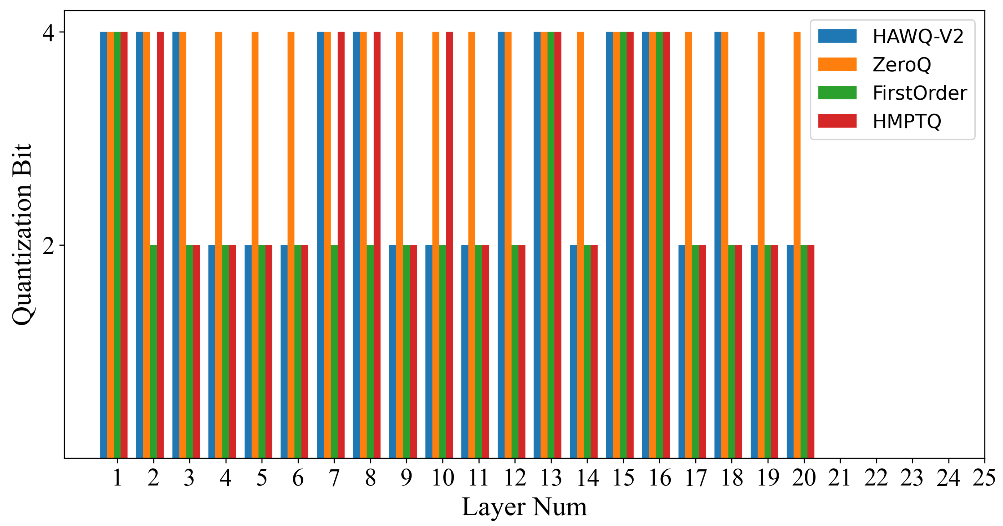
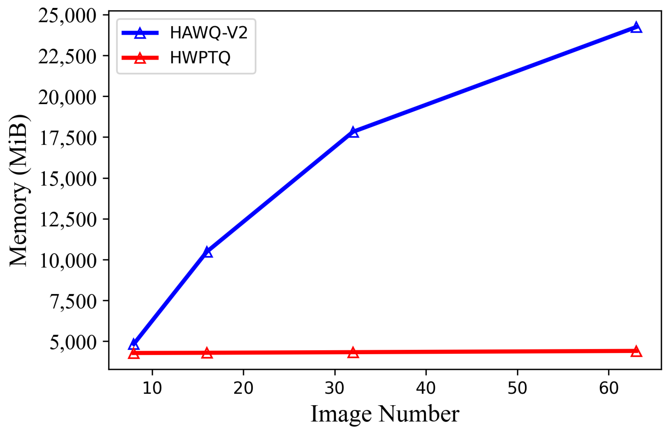
4.3.2. Experiments on Different Precision Allocation Methods

To evaluate the proposed reconstruction error-based layerwise precision configuration, Table 3 presents a detailed comparison of the YOLOV5n performance with the SSDD, HRSID, and LS-SSDD-v1.0 datasets using various configuration methods, including HAWQ-V2 [20], ZeroQ [21], and FirstOrder [29]. In these methods, each layer’s quantization utilizes the proposed intra-layer mixed-precision quantization.

Table 3. Comparison results of our proposed reconstruction error-based precision configuration method and state-of-the-art precision evaluation method for YOLOV5n on the SSDD, HRSID, and LS-SSDD-v1.0 datasets. The symbol ↓ indicates a decrease.

		SSDD				HRSID				LS-SSDD-v1.0
Method	Bits	Params	mAP	Params↓	$\Delta$mAP	Params	mAP	Params↓	$\Delta$mAP	Params	mAP	Params↓	$\Delta$mAP
	(W/A)	(MB)	(%)	(%)	(%)	(MB)	(%)	(%)	(%)	(MB)	(%)	(%)	(%)
Baseline	FP32	7.04	98.21	-	-	7.04	92.21	-	-	7.04	75.48	-	-
HAWQ−V2 [20]	WP84A8	1.68	98.17	76.17	−0.04	1.68	92.11	76.19	−0.10	1.61	72.79	77.12	−2.69
HAWQ−V2 [20]	WP42A8	1.15	98.34	83.73	0.13	1.15	91.93	83.67	−0.28	1.12	72.45	84.12	−3.03
ZeroQ [21]	WP84A8	1.68	97.46	76.09	−0.75	1.68	92.07	76.19	−0.14	1.69	72.92	75.93	−2.56
ZeroQ [21]	WP42A8	1.18	78.24	83.22	−19.97	1.19	26.58	83.11	−65.63	1.09	63.51	84.57	−11.97
FirstOrder [29]	WP84A8	1.71	98.38	75.76	0.17	1.67	92.16	76.24	−0.05	1.67	73.39	76.26	−2.09
FirstOrder [29]	WP42A8	1.16	98.00	83.49	−0.21	1.16	92.01	83.52	−0.20	1.14	71.81	83.76	−3.67
HMPTQ	WP84A8	1.62	98.27	77.04	0.06	1.67	92.19	76.28	−0.02	1.67	73.39	76.26	−2.09
HMPTQ	WP42A8	1.13	98.38	84.01	0.17	1.14	92.07	83.80	−0.14	1.14	73.53	83.88	−1.93

(1) Results

Table 3 compares the performance of YOLOV5n on the SSDD, HRSID, and LS-SSDD-v1.0 datasets using different quantization methods like HAWQ-V2, ZeroQ, and FirstOrder. Each method utilizes the proposed intra-layer mixed-precision quantization for efficient model compression.

Using the HAWQ-V2 method with the WP84A8 configuration, the parameter size is reduced to 1.68 MB, achieving mAP values of 98.17%, 92.11%, and 72.79% on the SSDD, HRSID, and LS-SSDD-v1.0 datasets, with mAP changes ranging from −0.04% to −2.69%. The WP42A8 configuration further reduces the parameter size to 1.15 MB (an 83.73% reduction), producing mAP values of 98.34%, 91.93%, and 72.45%, with mAP changes between −0.28% and 0.13%.

On the other hand, the ZeroQ method with the WP84A8 configuration also reduces the parameter size to 1.68MB (a 76.09% reduction). However, mAP values drop to 97.46%, 92.07%, and 72.92%, with mAP changes between −0.75% and −2.56%. The WP42A8 configuration reduces the parameter size to 1.18 MB (an 83.22% reduction), but mAP values significantly decline to 78.24%, 26.58%, and 63.51%, with drastic mAP changes ranging from −65.63% to −11.97%.

For the FirstOrder method, the WP84A8 configuration reduces the parameter size to 1.71 MB (a 75.76% reduction) and achieves mAP values of 98.38%, 92.16%, and 73.39%, with mAP changes between 0.17% and −2.09%. The WP42A8 configuration reduces the parameter size to 1.16 MB (an 83.49% reduction), yielding mAP values of 98.00%, 92.01%, and 71.81%, with mAP changes of −0.21%, −0.20%, and −3.67%.

The proposed method performs better across all datasets. With the WP84A8 configuration, it reduces the parameter size to 1.62 MB (a 77.04% reduction) and achieves mAP values of 98.27%, 92.19%, and 73.39%, with minimal mAP changes from −0.02% to 0.06%. The WP42A8 configuration further reduces the parameter size to 1.13 MB (an 84.01% reduction), yielding mAP values of 98.38%, 92.07%, and 73.53%, with mAP changes ranging from −0.14% to 0.17%.

(2) Discussion

The evaluation results demonstrate that the proposed reconstruction error-based layerwise precision configuration offers significant advantages in both parameter reduction and accuracy retention compared to existing methods like HAWQ-V2, ZeroQ, and FirstOrder. While HAWQ-V2 achieves moderate parameter reduction with stable mAP performance, it falls short in compression efficiency compared to the proposed method. Notably, the WP42A8 configuration in HAWQ-V2 shows only slight mAP improvements, indicating a limit in balancing compression and performance.

ZeroQ, despite achieving comparable parameter reductions, suffers from significant performance degradation, especially in the WP42A8 configuration, where mAP values drop substantially across all datasets. This shows that ZeroQ is less robust when subjected to aggressive quantization, leading to notable accuracy losses, particularly on the more complex LS-SSDD-v1.0 dataset.

FirstOrder demonstrates better mAP stability than ZeroQ, particularly in the WP84A8 configuration, where it achieves competitive accuracy across all datasets. However, like HAWQ-V2, FirstOrder lags behind the proposed method in compression efficiency, particularly in the balance between parameter reduction and mAP performance. This suggests that while FirstOrder performs well, its layerwise precision configuration lacks the refinement needed to match the compression gains of the proposed method.

The proposed method stands out by significantly reducing parameter sizes without compromising accuracy. Its WP84A8 and WP42A8 configurations not only achieve competitive mAP values but also better preserve accuracy across all datasets. The ability to maintain mAP values close to or better than those achieved by HAWQ-V2 and FirstOrder, while significantly outperforming ZeroQ, highlights the effectiveness of the proposed intra-layer mixed-precision quantization strategy.

The additional analysis in Figure 7 and Figure 8 further emphasizes the benefits of the proposed approach. The stable memory requirements associated with the reconstruction error-based method, even as the number of images increases, indicate lower computational costs compared to the Hessian trace computation required by other methods. This makes the proposed method more suitable for large-scale applications, where computational efficiency and scalability are critical.

Figure 7. Weight quantization to 4-bit or 2-bit for select layers in the pre-trained YOLOV5n model on the SSDD dataset.

Figure 8. Comparison of memory requirements for Hessian trace computation and reconstruction error of HMPTQ.

In summary, the proposed method effectively balances model compression and accuracy retention, offering substantial improvements over existing methods. The combination of high mAP values and significant parameter reductions suggests that the method can be effectively applied in resource-constrained environments, such as edge devices, without sacrificing performance.

5. Conclusions

In this paper, we introduced the HMPTQ method designed to effectively compress models for SAR ship detection using CNNs. The HMPTQ method minimizes quantization errors through careful layerwise precision configurations and mixed-precision strategies within layers. This approach achieves substantial reductions in model size while maintaining high accuracy. Our experimental results demonstrate that HMPTQ outperforms existing approaches across various datasets. The method not only reduces the number of parameters but also maintains detection accuracy with minimal loss, showing improvements in some cases. These findings emphasize the practical value of HMPTQ in resource-constrained environments and lay a foundation for extending this method to broader neural network architectures and datasets. However, HMPTQ is primarily optimized for CNNs. When applied to architectures that incorporate non-convolutional components, such as transformers or hybrid models, the standard quantization strategy may require further adaptation. Exploring additional datasets and varying conditions—such as different resolutions or satellite data—would provide a more comprehensive evaluation of our method. We identify this as an important direction for future research. Future work will also focus on further validating the robustness and adaptability of HMPTQ across practical applications. This includes extending the methodology to various neural network architectures and datasets, demonstrating its robustness in a wide range of real-world scenarios.

References

1. Chen, S.; Zhan, R.; Wang, W.; Zhang, J. Learning Slimming SAR Ship Object Detector Through Network Pruning and Knowledge Distillation. IEEE J. Sel. Top. Appl. Earth Observ. Remote Sens. 2021, 14, 1267–1282. [Google Scholar] [CrossRef]
2. Ma, X.; Ji, K.; Xiong, B.; Zhang, L.; Feng, S.; Kuang, G. Light-YOLOv4: An Edge-Device Oriented Target Detection Method for Remote Sensing Images. IEEE J. Sel. Top. Appl. Earth Observ. Remote Sens. 2021, 14, 10808–10820. [Google Scholar] [CrossRef]
3. Yang, Y.; Lang, P.; Yin, J.; He, Y.; Yang, J. Data Matters: Rethinking the Data Distribution in Semi-Supervised Oriented SAR Ship Detection. Remote Sens. 2024, 16, 2551. [Google Scholar] [CrossRef]
4. Jeon, H.; Kim, D.j.; Kim, J. Water Body Detection using Deep Learning with Sentinel-1 SAR satellite data and Land Cover Maps. In Proceedings of the 2021 IEEE International Geoscience and Remote Sensing Symposium (IGARSS), Brussels, Belgium, 11–16 July 2021; pp. 8495–8498. [Google Scholar]
5. Wang, Z.; Zhang, R.; Zhang, Q.; Zhu, Y.; Huang, B.; Lu, Z. An Automatic Thresholding Method for Water Body Detection from SAR Image. In Proceedings of the 2019 IEEE International Conference on Signal, Information and Data Processing (ICSIDP), Chongqing, China, 11–13 December 2019; pp. 1–4. [Google Scholar]
6. Yadav, R.; Nascetti, A.; Ban, Y. Attentive Dual Stream Siamese U-Net for Flood Detection on Multi-Temporal Sentinel-1 Data. In Proceedings of the 2022 IEEE International Geoscience and Remote Sensing Symposium (IGARSS), Kuala Lumpur, Malaysia, 17–22 July 2022; pp. 5222–5225. [Google Scholar]
7. Baghermanesh, S.S.; Jabari, S.; McGrath, H. Urban Flood Detection Using Sentinel1-A Images. In Proceedings of the 2021 IEEE International Geoscience and Remote Sensing Symposium (IGARSS), Brussels, Belgium, 11–16 July 2021; pp. 527–530. [Google Scholar]
8. Yang, Y.J.; Singha, S.; Mayerle, R. Fully Automated Sar Based Oil Spill Detection Using Yolov4. In Proceedings of the 2021 IEEE International Geoscience and Remote Sensing Symposium (IGARSS), Brussels, Belgium, 11–16 July 2021; pp. 5303–5306. [Google Scholar]
9. Xu, F.Y.; An, X.Z.; Liu, W.Q. Oil Spill Detection in SAR Images based on Improved YOLOX-S. In Proceedings of the 2022 International Conference on Computer Engineering and Artificial Intelligence (ICCEAI), Shijiazhuang, China, 22–24 July 2022; pp. 261–265. [Google Scholar]
10. Li, C.; Yang, Y.; Yang, X.; Chu, D.; Cao, W. A Novel Multi-Scale Feature Map Fusion for Oil Spill Detection of SAR Remote Sensing. Remote Sens. 2024, 16, 1684. [Google Scholar] [CrossRef]
11. Tan, J.; Tang, Y.; Liu, B.; Zhao, G.; Mu, Y.; Sun, M.; Wang, B. A Self-Adaptive Thresholding Approach for Automatic Water Extraction Using Sentinel-1 SAR Imagery Based on OTSU Algorithm and Distance Block. Remote Sens. 2023, 15, 2690. [Google Scholar] [CrossRef]
12. Ji, K.; Leng, X.; Wang, H.; Zhou, S.; Zou, H. Ship detection using weighted SVM and M-CHI decomposition in compact polarimetric SAR imagery. In Proceedings of the 2017 IEEE International Geoscience and Remote Sensing Symposium (IGARSS), Fort WOrth, TX, USA, 23–28 July 2017; pp. 890–893. [Google Scholar]
13. Fang, J.; Shafiee, A.; Abdel-Aziz, H.; Thorsley, D.; Georgiadis, G.; Hassoun, J. Post-training Piecewise Linear Quantization for Deep Neural Networks. In Proceedings of the European Conference on Computer Vision, Glasgow, UK, 23–28 August 2020. [Google Scholar]
14. Nagel, M.; Amjad, R.A.; van Baalen, M.; Louizos, C.; Blankevoort, T. Up or Down? Adaptive Rounding for Post-Training Quantization. arXiv 2020, arXiv:abs/2004.10568. [Google Scholar]
15. Lin, C.; Peng, B.; Li, Z.; Tan, W.; Ren, Y.; Xiao, J.; Pu, S. Bit-shrinking: Limiting Instantaneous Sharpness for Improving Post-training Quantization. In Proceedings of the 2023 IEEE Conference on Computer Vision and Pattern Recognition (CVPR), Vancouver, BC, Canada, 17–24 June 2023; pp. 16196–16205. [Google Scholar]
16. Jacob, B.; Kligys, S.; Chen, B.; Zhu, M.; Tang, M.; Howard, A.G.; Adam, H.; Kalenichenko, D. Quantization and Training of Neural Networks for Efficient Integer-Arithmetic-Only Inference. In Proceedings of the 2018 IEEE Conference on Computer Vision and Pattern Recognition (CVPR), Salt Lake City, UT, USA, 18–23 June 2018; pp. 2704–2713. [Google Scholar]
17. Kwak, J.; Kim, K.; Lee, S.S.; Jang, S.J.; Park, J. Quantization Aware Training with Order Strategy for CNN. In Proceedings of the IEEE Conference on Consumer Electronics-Asia, Yeosu, Republic of Korea, 26–28 October 2022; pp. 1–3. [Google Scholar]
18. Shen, M.; Liang, F.; Gong, R.; Li, Y.; Li, C.; Lin, C.; Yu, F.; Yan, J.; Ouyang, W. Once Quantization-Aware Training: High Performance Extremely Low-bit Architecture Search. In Proceedings of the IEEE Conference on Computer Vision, Montreal, QC, Canada, 10–17 October 2021; pp. 5320–5329. [Google Scholar]
19. Dong, Z.; Yao, Z.; Gholami, A.; Mahoney, M.; Keutzer, K. HAWQ: Hessian AWare Quantization of Neural Networks with Mixed-Precision. In Proceedings of the IEEE Conference on Computer Vision and Pattern Recognition (CVPR), Seoul, Republic of Korea, 27 Octobe–2 November 2019; pp. 293–302. [Google Scholar]
20. Dong, Z.; Yao, Z.; Arfeen, D.; Gholami, A.; Mahoney, M.W.; Keutzer, K. HAWQ-V2: Hessian Aware trace-Weighted Quantization of Neural Networks. In Proceedings of the Neural Information Processing Systems, Vancouver, BC, Canada, 6–12 December 2020. [Google Scholar]
21. Cai, Y.; Yao, Z.; Dong, Z.; Gholami, A.; Mahoney, M.W.; Keutzer, K. ZeroQ: A Novel Zero Shot Quantization Framework. In Proceedings of the IEEE Conference on Computer Vision and Pattern Recognition (CVPR), Seattle, WA, USA, 13–19 June 2020; pp. 13166–13175. [Google Scholar]
22. Wu, D.; Tang, Q.; Zhao, Y.; Zhang, M.; Fu, Y.; Zhang, D. EasyQuant: Post-training Quantization via Scale Optimization. arXiv 2020, arXiv:abs/2006.16669. [Google Scholar]
23. Choukroun, Y.; Kravchik, E.; Yang, F.; Kisilev, P. Low-bit Quantization of Neural Networks for Efficient Inference. In Proceedings of the IEEE Conference on Computer Vision and Pattern Recognition Workshops, Seoul, Republic of Korea, 27–28 October 2019; pp. 3009–3018. [Google Scholar]
24. Guan, H.; Malevich, A.; Yang, J.; Park, J.; Yuen, H. Post-Training 4-bit Quantization on Embedding Tables. arXiv 2019, arXiv:abs/1911.02079. [Google Scholar]
25. Oh, J.; Lee, S.; Park, M.; Walagaurav, P.; Kwon, K. Weight Equalizing Shift Scaler-Coupled Post-training Quantization. arXiv 2020, arXiv:abs/2008.05767. [Google Scholar]
26. Hubara, I.; Nahshan, Y.; Hanani, Y.; Banner, R.; Soudry, D. Improving Post Training Neural Quantization: Layer-wise Calibration and Integer Programming. arXiv 2020, arXiv:abs/2006.10518. [Google Scholar]
27. Li, Y.; Gong, R.; Tan, X.; Yang, Y.; Hu, P.; Zhang, Q.; Yu, F.; Wang, W.; Gu, S. BRECQ: Pushing the Limit of Post-Training Quantization by Block Reconstruction. arXiv 2021, arXiv:abs/2102.05426. [Google Scholar]
28. Wei, X.; Gong, R.; Li, Y.; Liu, X.; Yu, F. QDrop: Randomly Dropping Quantization for Extremely Low-bit Post-Training Quantization. arXiv 2022, arXiv:abs/2203.05740. [Google Scholar]
29. Chauhan, A.; Tiwari, U.; R, V.N. Post Training Mixed Precision Quantization of Neural Networks using First-Order Information. In Proceedings of the 2023 IEEE/CVF International Conference on Computer Vision Workshops (ICCVW), Paris, France, 2–6 October 2023; pp. 1335–1344. [Google Scholar]
30. He, K.; Zhang, X.; Ren, S.; Sun, J. Deep Residual Learning for Image Recognition. In Proceedings of the IEEE Conference on Computer Vision and Pattern Recognition, Las Vegas, NV, USA, 27–30 June 2016; pp. 770–778. [Google Scholar]
31. Zhang, T.; Zhang, X.; Li, J.; Xu, X.; Wang, B.; Zhan, X.; Xu, Y.; Ke, X.; Zeng, T.; Su, H.; et al. SAR Ship Detection Dataset (SSDD): Official Release and Comprehensive Data Analysis. Remote Sens. 2021, 13, 3690. [Google Scholar] [CrossRef]
32. Zhang, W.; Cai, M.; Zhang, T.; Zhuang, Y.; Mao, X. EarthGPT: A Universal Multimodal Large Language Model for Multisensor Image Comprehension in Remote Sensing Domain. IEEE Trans. Geosci. Remote Sens. 2024, 62, 1–20. [Google Scholar] [CrossRef]
33. Zhang, W.; Cai, M.; Zhang, T.; Zhuang, Y.; Mao, X. EarthMarker: A Visual Prompt Learning Framework for Region-level and Point-level Remote Sensing Imagery Comprehension. arXiv 2024, arXiv:abs/2407.13596. [Google Scholar]
34. Chen, Z.; Gao, X. An Improved Algorithm for Ship Target Detection in SAR Images Based on Faster R-CNN. In Proceedings of the 2018 Ninth International Conference on Intelligent Control and Information Processing (ICICIP), Wanzhou, China, 9–11 November 2018; pp. 39–43. [Google Scholar]
35. Chai, B.; Chen, L.; Shi, H.; He, C. Marine Ship Detection Method for SAR Image Based on Improved Faster RCNN. In Proceedings of the 2021 SAR in Big Data Era (BIGSARDATA), Nanjing, China, 22–24 September 2021; pp. 1–4. [Google Scholar]
36. Redmon, J.; Divvala, S.; Girshick, R.; Farhadi, A. You Only Look Once: Unified, Real-Time Object Detection. In Proceedings of the 2016 IEEE Conference on Computer Vision and Pattern Recognition (CVPR), Las Vegas, NV, USA, 27–30 June 2016; pp. 779–788. [Google Scholar]
37. Wang, H.; Wu, B.; Wu, Y.; Zhang, S.; Mei, S.; Liu, Y. An Improved YOLO-v3 Algorithm for Ship Detection in SAR Image Based on K-means++ with Focal Loss. In Proceedings of the 2022 3rd China International SAR Symposium (CISS), Shanghai, China, 2–4 November 2022; pp. 1–5. [Google Scholar]
38. Ting, L.; Baijun, Z.; Yongsheng, Z.; Shun, Y. Ship Detection Algorithm based on Improved YOLO V5. In Proceedings of the 2021 6th International Conference on Automation, Control and Robotics Engineering (CACRE), Dalian, China, 15–17 July 2021; pp. 483–487. [Google Scholar]
39. Ge, R.; Mao, Y.; Li, S.; Wei, H. Research On Ship Small Target Detection In SAR Image Based On Improved YOLO-v7. In Proceedings of the 2023 International Applied Computational Electromagnetics Society Symposium (ACES-China), Hangzhou, China, 15–18 August 2023; pp. 1–3. [Google Scholar]
40. Congan, X.; Hang, S.; Jianwei, L.; Yu, L.; Libo, Y.; Long, G.; Wenjun, Y.; Taoyang, W. RSDD-SAR: Rotated Ship Detection Dataset in SAR Images. J. Radars 2022, 11, 581. [Google Scholar]
41. Sandler, M.; Howard, A.; Zhu, M.; Zhmoginov, A.; Chen, L.C. MobileNetV2: Inverted Residuals and Linear Bottlenecks. In Proceedings of the IEEE Conference on Computer Vision and Pattern Recognition (CVPR), Salt Lake City, UT, USA, 18–23 June 2018; pp. 4510–4520. [Google Scholar]
42. Wei, S.; Zeng, X.; Qu, Q.; Wang, M.; Su, H.; Shi, J. HRSID: A High-Resolution SAR Images Dataset for Ship Detection and Instance Segmentation. IEEE Access 2020, 8, 120234–120254. [Google Scholar] [CrossRef]
43. Zhang, T.; Zhang, X.; Ke, X.; Zhan, X.; JUN, S.; Wei, S.; Pan, D.; Li, J.; Su, H.; Zhou, Y.; et al. LS-SSDD-v1.0: A deep learning dataset dedicated to small ship detection from large-scale Sentinel-1 SAR images. Remote Sens. 2020, 12, 2997. [Google Scholar] [CrossRef]
44. Ultralytics. YOLOv5. Available online: https://github.com/ultralytics/yolov5 (accessed on 26 June 2020).
45. Wang, C.Y.; Yeh, I.H.; Liao, H. YOLOv9: Learning What You Want to Learn Using Programmable Gradient Information. arXiv 2024, arXiv:abs/2402.13616. [Google Scholar]
Disclaimer/Publisher’s Note: The statements, opinions and data contained in all publications are solely those of the individual author(s) and contributor(s) and not of MDPI and/or the editor(s). MDPI and/or the editor(s) disclaim responsibility for any injury to people or property resulting from any ideas, methods, instructions or products referred to in the content.
Article Metrics
Citations
Article Access Statistics
Multiple requests from the same IP address are counted as one view.