Article

Bidirectional Feature Fusion and Enhanced Alignment Based Multimodal Semantic Segmentation for Remote Sensing Images

School of Computer Science, Shaanxi Normal University, Xi’an 710119, China
*
Author to whom correspondence should be addressed.
Remote Sens. 2024, 16(13), 2289; https://doi.org/10.3390/rs16132289
Submission received: 25 April 2024 / Revised: 20 June 2024 / Accepted: 20 June 2024 / Published: 22 June 2024
(This article belongs to the Special Issue Image Processing from Aerial and Satellite Imagery)

Abstract

:
Image–text multimodal deep semantic segmentation leverages the fusion and alignment of image and text information and provides more prior knowledge for segmentation tasks. It is worth exploring image–text multimodal semantic segmentation for remote sensing images. In this paper, we propose a bidirectional feature fusion and enhanced alignment-based multimodal semantic segmentation model (BEMSeg) for remote sensing images. Specifically, BEMSeg first extracts image and text features by image and text encoders, respectively, and then the features are provided for fusion and alignment to obtain complementary multimodal feature representation. Secondly, a bidirectional feature fusion module is proposed, which employs self-attention and cross-attention to adaptively fuse image and text features of different modalities, thus reducing the differences between multimodal features. For multimodal feature alignment, the similarity between the image pixel features and text features is computed to obtain a pixel–text score map. Thirdly, we propose a category-based pixel-level contrastive learning on the score map to reduce the differences among the same category’s pixels and increase the differences among the different categories’ pixels, thereby enhancing the alignment effect. Additionally, a positive and negative sample selection strategy based on different images is explored during contrastive learning. Averaging pixel values across different training images for each category to set positive and negative samples compares global pixel information while also limiting sample quantity and reducing computational costs. Finally, the fused image features and aligned pixel–text score map are concatenated and fed into the decoder to predict the segmentation results. Experimental results on the ISPRS Potsdam, Vaihingen, and LoveDA datasets demonstrate that BEMSeg is superior to comparison methods on the Potsdam and Vaihingen datasets, with improvements in mIoU ranging from 0.57% to 5.59% and 0.48% to 6.15%, and compared with Transformer-based methods, BEMSeg also performs competitively on LoveDA dataset with improvements in mIoU ranging from 0.37% to 7.14%.

1. Introduction

Semantic segmentation as a pixel-level classification task assigns semantic category labels to each pixel in the image. It is an important means of achieving automatic interpretation of remote sensing images and provides the basis for many remote sensing applications, such as land cover [1], military target detection [2], earthquake landslide detection [3], urban ecological research [4], etc. With the rapid advancement of deep learning, semantic segmentation networks, including convolutional neural networks, recurrent neural networks, and adversarial neural networks have become mainstream in image semantic segmentation research. The semantic segmentation model is mainly based on the encoder–decoder [5] structure, applying multi-scale feature fusion [6], feature pyramid network [7], attention mechanism [8], Transformer [9], and other technologies [10] to better extract features and achieve refined segmentation.
Previous research on image semantic segmentation was mainly based on image information and supervised learning. In recent years, vision-language pretraining (VLP) models have provided a novel learning paradigm combining different text and image modalities, using multimodal information to extract more general features on large-scale labeled training sets. The models can be applied to unlabeled data and transferred to various downstream visual tasks such as image classification, segmentation, and target detection, which has garnered interest from researchers. In 2021, Radford et al. [11] proposed the CLIP model using large-scale image-caption pairs as training data, mapping the global features of the image and the text features of the caption to a unified feature space. By similarity computation and contrastive learning, the CLIP pretraining model achieves image-level classification tasks by aligning multimodal features, novel ideas, and significant effects to facilitate the expansion of image–text multimodal research into semantic segmentation tasks.
The research on image–text multimodal deep semantic segmentation is mainly based on the encoder–decoder network structure. Text and image features are extracted through a text encoder and an image encoder respectively, and both two kinds of features are fused and aligned, and then provided for the image decoder to obtain the pixels’ category prediction. In feature extraction, existing methods have adopted different ways to obtain feature representations of different modalities, including directly applying the image and text encoder structure and its parameters in the pretraining model [12,13,14,15]; proposing a new encoder structure [16]; and adjusting the input of the feature encoder by prompt learning [17,18]. With the introduction of more natural language processing (NLP) models and image semantic segmentation models, many advanced feature extraction networks can be used directly. Determining how to construct the interactive connections between multimodal features is the current focus of research. Multimodal feature fusion integrates features from different modalities to obtain a more comprehensive and accurate representation, thereby improving the model’s understanding ability to multimodal data. After obtaining the image and text features, the interaction between the image and text features is established through multimodality fusion technology (MFT) [19]. Current MFTs achieve unidirectional feature fusion for the text-to-image or image-to-text, such as the multimodal cross-attention network [20], feature transformation [18], and attention mechanism in the Transformer decoder [13]. However, these methods only adapt to a single modality of image or text and lack the flexibility to adjust to both the image and text feature features simultaneously.
To define the relationship between different modalities, multimodal feature alignment performs semantic matching and computes the similarity between different modal features to better learn features. For image–text dense semantic segmentation, two methods are usually adopted to achieve feature alignment: one involves encoding the pixel features within the image and category text features into a unified feature space, and computing the similarity between the two features by the dot product. The dot product results between pixel features and text features (i.e., pixel–text score map) determine the matching degree of pixel and text. However, the pixel–text score map only considers the similarity between a single pixel and the category text, ignoring the relationship between different pixels. The other involves grouping or clustering the pixels in the image to obtain region features, and using contrastive learning to increase the similarity of region and text features of the same category and reduce that of different categories. However, the process of grouping image features or predicting region masks takes a lot of time and memory space, and the quality of the mask will also affect the final semantic segmentation result. After multimodal feature fusion and alignment, the aligned pixel–text score map, the multimodal fused image feature, or the pixel–text score map and image feature are concatenated by channel [21] and are fed into the decoder to achieve segmentation prediction.
Remote sensing images are characterized by complex backgrounds, multi-scale ground objects, and the “same objects with different spectra, different objects with similar spectra”, which increases the difficulty of feature extraction in semantic segmentation methods. In addition, the label acquisition of remote sensing images is time-consuming and laborious, which hinders the improvement of single-modal image-supervised models for remote sensing applications. At present, the single-modal semantic segmentation for remote sensing images faces three challenges: first, because of the phenomenon of the “same objects with different spectra, different objects with similar spectra” in remote sensing images, it is difficult to achieve accurate segmentation only by image spectral features. Secondly, remote sensing images pose a challenge for feature representation and distinction of different classes due to the problem of large intra-class variance and small inter-class variance. Additionally, the number of different classes’ pixels in remote sensing images is usually different (i.e., class imbalance problem), and deep networks need to crop the original large-scale image to a smaller size as input. Because the number of pixels in some categories is too small, these categories easily disappear in the cropped input image, resulting in degradation segmentation performance. The image–text multimodal models show great potential in computer visual tasks. In the remote sensing field, combining the fusion and alignment of multimodal text and image features can provide more prior knowledge for semantic segmentation for remote sensing images. This type of research is expected to provide new methods that can better meet the needs of practical applications and is worth exploring [22].
In response to the above challenges, this paper proposes a bidirectional feature fusion and enhanced alignment-based multimodal semantic segmentation (BEMSeg) model for remote sensing images. The model consists of three parts: encoding, multimodal feature fusion and alignment, and decoding. Firstly, a text encoder and an image encoder are used for feature extraction. Then a bidirectional feature fusion (BFF) module is proposed to realize multimodal feature fusion. To facilitate multimodal feature alignment, we propose a category-based pixel-level contrastive (CPC) learning on the alignment pixel–text score map; finally, the pixel–text score map is concatenated with the image features and fed into the decoder to predict segmentation results. Experimental results show the BEMSeg effectively improved performance on the semantic segmentation for remote sensing images. The main contributions of this paper include three aspects:
  • This paper proposes a BFF module based on self-attention and cross-attention to maintain the completeness of single-modal semantic information while realizing the complementarity of image–text multimodal features.
  • The CPC learning is proposed on the pixel–text score map obtained by feature alignment to reduce the difference among the pixels of the same category and increase the gap among pixels of different categories.
  • A selection strategy for positive and negative samples is proposed, expanding the CPC learning to different images and making full use of the global semantic features of pixels.
This article is organized as follows. Section 2 introduces related work on multimodal semantic segmentation. Section 3 details the proposed model. The experimental setup and results analysis are presented in Section 4. Finally, Section 5 provides the conclusion of this paper.

2. Related Work

The success of CLIP [11] and ALIGN [23] inspired a series of research on combining image–text multimodal information to achieve computer vision tasks. Currently, the image–text multimodal semantic segmentation models adopt an encoder–decoder network structure, after feature extraction, the image features and text features are fused and aligned, and the aligned features are input into the decoding together with image features to predict the category of each pixel. The research focuses involve of feature encoding, multimodal feature fusion and alignment, and feature decoding. Different semantic segmentation models have been studied for each focus, which are introduced and analyzed below.

2.1. Feature Encoding

The image–text multimodal semantic segmentation models utilize a text encoder and an image encoder to extract text features and image features respectively. Image features are usually extracted by existing backbone networks based on pretraining CLIP weights, such as ResNet 50, ResNet 101, ViT-L/16 [13,15,18], and masked autoencoder pre-trained ViT [14,24]. Text features are usually extracted by the text encoder provided by CLIP-ViT-B/32 [15] or the BERT-Large model [12].
To adapt pretraining models to specific downstream segmentation tasks, some works finetuning CLIP encoder, the knowledge of the CLIP model is preserved as much as possible by setting a small learning rate. Other works freeze the pretraining encoder while introducing a set of trainable parameters in each layer of the Transformer encoder [25] or an additional bottleneck layer to learn new task-specific features [26]. To better learn text features, inspired by the ‘promote’ project in the NLP tasks, Zhou et al. [17] proposed setting up learnable context prompt variables to replace manually designed prompt variables, which are concatenated with text vectors as the input to the text encoder. In addition, some works retrained the newly established encoder to adapt specific segmentation tasks, such as GroupViT [16], which requires a substantial amount of training data and a large-scale model. In our study, we apply a fine-tuning image encoder in the pretraining CLIP model while setting learnable context variables in the text encoder, thus enhancing the feature extraction capability for remote sensing semantic segmentation tasks.

2.2. Image–Text Information Fusion and Alignment

Text and image information are heterogeneous and complementary, using features of different modalities is beneficial to obtain more expressive and discriminative features for category prediction, thereby improving model performance [27]. Multimodal information fusion is classified as feature-level fusion and decision-level fusion according to whether features or predictions are fused to obtain a more comprehensive feature representation or prediction. In feature-level multimodal feature fusion, some technologies such as feature concatenate, cross-attention, and feature transformation are introduced in semantic segmentation models. Certain works concatenated the extracted image features and text features to obtain a new image–text fusion feature and then passed them into an attention mechanism [20] or convolution layer [28] to explore fusion information. These methods blend the information between multimodality and ignore the completeness of each single modal.
To integrate text features into image features, Luddecke and Ecker [18] used feature-wise linear modulation (FiLM) [29] to transform the text features into scaling and shifting vectors, which are multiplied and added to the image features to obtain the fused image features. To integrate image features into text features, Rao et al. [13] incorporated both image and text features into a cross-attention module [30], which encourages the text features to find the most related visual clues and updates them through the residual connection between the learned output sequence and text features. These two multimodal fusion technologies only apply an affine transformation to one modality’s features, without considering the interaction between multimodal features. Therefore, we propose a BFF module that uses a self-attention mechanism to model relationships within modalities and uses the bidirectional cross-attention mechanism to realize image-to-text and text-to-image feature fusion.
Different from multimodal feature fusion, multimodal feature alignment facilitates joint learning of different modalities by establishing a correspondence between two different modal features, which can be achieved through matching and mapping [27,31]. Matching is an alignment manner with a similarity hierarchy, achieved by enhancing the similarity between two modal features of the same category, and mapping usually represents logical equivalence or inclusion relationships between different modal features. In multimodal image classification, the CLIP [11] and ALIGN [23] models encoded global image features and text features into the shared feature space and achieved matching alignment by computing the similarity of the two features. In the segmentation task, the pixel features or masked image features are encoded into a shared feature space with text features to achieve alignment. DenseCLIP [13] and LSeg [15] encoded image pixel features and text features and computed the similarity between pixels and text features through dot product, thereby achieving pixel–text matching. GroupViT [16] utilized pixel grouping and contrastive learning between learned image group features and text features to achieve multimodal feature alignment. OpenSeg [12] and MAFT [32] predicted mask proposals of the image and used masked image features and text word features to achieve feature alignment.
However, mask prediction, pixel clustering, or grouping during the image feature extraction takes up more computation resources and greatly influences the final segmentation result. While the pixel-text-based alignment methods compute the similarity between each independent pixel and the text feature, ignoring the long-range dependence between different pixels of the same category. Therefore, different from the above methods, we propose using contrastive learning of cross-images for pixel–text matching to establish long-range dependencies and enhance the alignment effect.

2.3. Feature Decoding

Feature decoding is applied to multi-scale image features and aligned multimodal features to achieve semantic segmentation prediction. In pixel–text matching, LSeg [15] firstly fused image features of different scales into a high-resolution feature map, and then aligned the feature map with the text features. The image feature map with high resolution and more channels in the multimodal feature alignment process may result in a relatively large amount of computation and memory. DenseCLIP [13] obtained the pixel–text score map from the alignment of high-level image semantic feature and text feature, and concatenated it with the high-level feature map, the final segmentation results are obtained through the fusion of multi-scale feature maps. Luddecke and Ecker [18] proposed a Transformer-based CLIPSeg decoder structure, used the multimodal fusion image feature as input, and skip-connected the extracted image features of the encoder to obtain the segmentation prediction results. However, CLIPSeg can only achieve binary segmentation prediction and cannot directly complete multi-classification. Similar to DenseCLIP, we utilize the image features and the pixel–text score map as the input of the feature decoding and apply the multi-scale feature fusion method in Semantic FPN [33] to achieve feature upsampling and segmentation result prediction.

3. Proposed Method

To integrate multimodal information to realize semantic segmentation for remote sensing images, this paper proposes a bidirectional feature fusion and enhanced alignment-based multimodal semantic segmentation (BEMSeg) model. The model’s framework is shown in Figure 1, which contains three parts: encoder, multimodal feature fusion and alignment, and decoder. First, a continuous learnable promote variable [17] is connected with the category text, inputting images and texts into the image encoder and text encoder to extract image features and text features respectively. Then the two modal features are input into the multimodal feature fusion and alignment part. In multimodal feature fusion, the bidirectional feature fusion (BFF) module based on the attention mechanism is proposed to fuse image and text features mutually. In multimodal feature alignment, using the dot product to align the fused image features and text features, the similarity between the pixel features and text features in the image is computed, and a pixel–text score map is obtained to capture the relationship between multimodalities. Finally, the obtained pixel–text score map is concatenated with the image features and fed into the decoder to predict the semantic segmentation results.
The pixel–text score map can be regarded as the prediction result at low resolution, which is used to compute the auxiliary segmentation loss with the label. To model the relationship among pixels after feature alignment, a category-based pixel-level contrastive (CPC) learning is proposed on the pixel–text score map to obtain the contrastive loss. These two losses and the predicted semantic segmentation results are used together with the segmentation loss computed by the real label as the final loss function to train the model.

3.1. Image–Text Bidirectional Feature Fusion

The BEMSeg model employs ResNet50 and a Transformer-based network with CLIP pretraining weights as the image encoder and text encoder, the extracted image features and text features are expressed as { x l R H l × W l × D l } l = 1 4 and q R C × D 4 , where x represents the image feature map, l indicates the number of layers, H, W, and D indicate the height, width and number of channels of the feature map respectively, C denotes the number of text categories, which is equal to the number of object categories in the image. To make full use of multimodal features to improve model performance, BEMSeg uses multimodal feature fusion to integrate image and text features. The learnable parameters are set as the inputs of the text encoder together with the category text words to learn the text knowledge related to remote sensing images. Through the fusion of image-context features with text features, the text is endowed with information about different remote sensing ground objects, enhancing the discriminability of the text features. Due to the diverse semantic information expressed in text, the fusion of text-to-image features is beneficial. It helps reduce the spectral differences within the same class and increase the spectral differences between different classes, thus alleviating the problem of “same object with different spectra, different objects with similar spectra”. For example, the similar spectral features between low vegetation and tree categories can be differentiated by fusing them with distinct text features for “low vegetation” and “tree”, which can increase the categorical differences in the image features, thereby improving the segmentation performance.
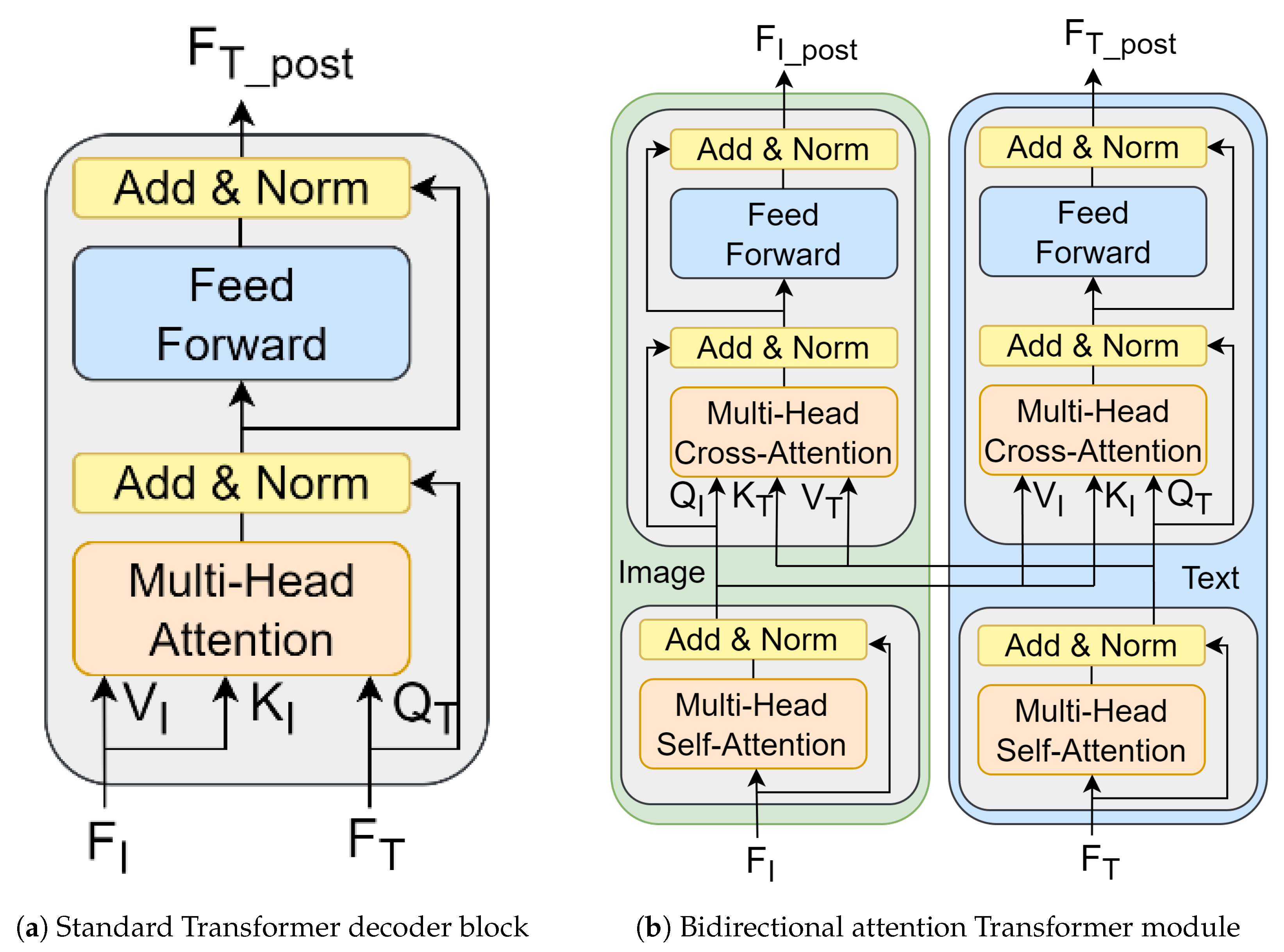
Considering the above problems, this paper proposes a bidirectional feature fusion (BBF) module that adapts to both image and text features, the module uses a self-attention and a bidirectional attention mechanism to achieve image-to-text and text-to-image feature fusion. The standard Transformer decoder block in Figure 2a, contains a multi-head attention layer and a fully connected network layer, both of which are followed by a residual connection and a normalization layer. The matrices V and K for one feature and the matrix Q for the other feature are the input of the multi-head attention layer, after the Transformer block, the attention feature is obtained. To achieve attention between different modal features, we input text features and image features into the multi-head cross-attention layer, modifying the key–value pairs to obtain the newly fused image and text features, thereby achieving bidirectional multimodal feature fusion. As shown in Figure 2b, the BBF module consists of image and text branches, and each branch contains a self-attention mechanism and a cross-attention mechanism. The image and text features before fusion are represented as F I and F T , respectively, and the image and text features obtained after fusion are represented as F I _ p o s t and F T _ p o s t , respectively.
To ensure the completeness and relevance of single-modal specific semantics, the self-attention mechanism is adopted to model the internal connections of image and text features, and effectively capture the global context information within the modality. In the self-attention mechanism, the input features and three trainable parameter matrices are used to obtain the query, key, and value matrices (e.g., Q, K, and V) through matrix multiplication. Self-attention is computed as Equation (1):
self-attention ( Q , K , V ) = s o f t m a x ( Q K T d k ) V
where K T and d k represent the transposed matrix of K and keys in K of dimension. Inputting image features and text features into the self-attention layer separately to learn the context relationship within each modality, then passing them into the cross-attention mechanism to achieve multimodal feature fusion. Different from the self-attention mechanism, Q, K, and V matrices in the cross-attention mechanism are derived from different input features. The matrices from image features are expressed as Q I , K I , and V I , and the matrices from text features are expressed as Q T , K T , and V T . The cross-attention mechanism in the image branch can be expressed as follows:
C r o s s A t t e n t i o n ( Q I , K T , V T ) = s o f t m a x ( Q I K T T d k ) V T
where Q I K T T represents the similarity between image features and text features. After applying a softmax activation function to it, the similarity coefficient matrix of each text feature and image feature is obtained. This coefficient matrix is multiplied by the value matrix V T of the text feature, and then the text-attention image features are obtained through weighted summation. The image features output by the cross-attention mechanism are residually connected to the input image features, and the multimodal fused image features are output through fully connected layers and normalization layers. In the text branch, using Q T , K I , and V I as the inputs of the cross-attention mechanism to obtain the image-attention text features.
After realizing bidirectional feature fusion, the extracted image and text features are adjusted through a residual connection as follows to ensure semantic richness:
v = x 4 + γ 1 x 4 _ p o s t t = q + γ 2 q _ p o s t
where x 4 and q represent the last layer of image features and the text features, x 4 _ p o s t and q _ p o s t represent image features and text features after bidirectional feature fusion, respectively. γ 1 and γ 2 denote the learnable parameters to control the scaling ratio of the residual and are initialized as a very small value (such as 10 4 ) to preserve the extracted image and text features, v and t denote the image and text features after the residual connection.
Compared with existing image–text multimodal semantic segmentation models, the BBF module not only uses a self-attention mechanism to maintain the semantic completeness of a single modality but also uses a cross-attention mechanism to achieve multimodal feature fusion. The BBF module adaptively adjusts image and text features to obtain a more comprehensive feature representation, reduces the difference between image and text features, and facilitates subsequent feature alignment between multimodalities. Compared with the collaborative attention Transformer layer in the visual question and answer task [34], we added a self-attention mechanism to the BBF module after the convolutional feature extraction network to capture the correlation within each modal feature and utilize a cross-attention mechanism to fuse different modal features. For the first time, BEMSeg applied a bidirectional cross-attention mechanism in the semantic segmentation task, adjusting feature representation through image–text multimodal feature fusion, which provided important support for subsequent multimodal feature alignment and semantic segmentation tasks.

3.2. Image–Text Feature Alignment

To establish the mutual semantic relationship between multimodalities and achieve feature alignment, the dot product as follows is used to compute the similarity between the high-level semantic pixel features and text features:
s = v ^ t ^ T
where v ^ and t ^ refer to the normalized features of v and t respectively, s R H 4 × W 4 × C represents the pixel–text score map that records the similarity score between each pixel and each category. Using normalization to constrain the values of features is beneficial to computing the similarity between multimodal features. In the feature alignment, each pixel feature is treated as an independent individual to compute the similarity with text features of all categories, the relationship among different pixels is easily ignored. The pixels that belong to the same category at different positions tend to have stronger dependencies. To model the semantic correlation between pixels in the pixel–text score map, we propose a CPC learning to promote the image–text feature alignment effect on the same category. The pixel–text score map is related to both image features and text features, and contrastive learning on it can involve multimodal information. Compared with the image feature map, the pixel–text score map has a smaller number of channels and therefore requires less computation cost. In addition, CPC learning is only used during training to align multimodal features.
In CPC learning, based on the maximum value of a pixel on its channel in the pixel–text score map, the predicted category to which the pixel belongs is obtained, pixels of the same category are used as positive samples, and pixels of different categories are used as negative samples. Then, the similarity between each pixel and the positive and negative samples is computed, and the long-range dependence between pixels is modeled by increasing the similarity among pixels of the same category and reducing the similarity among pixels of different categories. The contrastive loss function InfoNCE is defined as follows:
L i N C E = 1 P i i + P i log exp ( i · i + / η ) exp ( i · i + / η ) + i N i exp ( i · i / η )
where P i and N i represent the positive sample set and the negative sample set of the pixel i, respectively, i + and i represent the positive sample and the negative sample, respectively, and η is used to control the smoothness of the loss value. For η , a smaller value leads to a sharper loss distribution, while a larger value results in a smoother distribution. Referring to [35] set η = 0.1 .
However, downsampling and pooling operations lead to too few or absent pixels of certain categories in the extracted high-level image features, resulting in the lack of positive samples and negative samples especially when the classes of remote sensing images are imbalanced. To address this problem, this paper expands the scope of sample selection and uses pixels of the same category in different images as positive samples and pixels of the different categories in different images as negative samples for contrastive learning. The pixel information among different images is conducive to obtaining the global feature correlation in the training data set. Due to the excessive number of pixels in the entire training set, there are too many samples in category-based contrastive learning, which easily results in computational redundancy and has a relatively small contribution to gradient update. Therefore, we propose a positive and negative sample selection strategy based on different images, averaging the pixel information of different categories on each image, to set a fixed number of positive and negative samples in each iteration process for contrastive learning.
The specific sample selection process is as follows: assuming that the batch size is B, the pixel–text score map s b R H 4 × W 4 × C , b 1 , , B is obtained by aligning the image and text features. Then the pixel features of each category in s b are averaged to obtain the mean samples, which are represented as p b , c R 1 × C , c 1 , , C and C is the number of semantic categories. After averaging over all pixel–text score maps, a sample set S R B × C × C is obtained, and the sample set is dynamically updated as the iteration proceeds. For a certain category c, the number of mean samples from the same category in a batch is B and their channel number is C. For a certain pixel i, according to its category, the positive sample set and the negative sample set from the sample set S are denoted as P i R B × C and N i R B ( C 1 ) × C for contrastive learning. The contrastive loss for all pixels of the pixel–text score map is as follows:
L c o n = i = 1 H 4 W 4 L i N C E
where L i N C E is computed as Equation (5). In addition, the pixel–text score map corresponds to the similarity value of each pixel on each category, which can be regarded as the prediction result at low resolution, and the segmentation loss between the score map and the label can serve as an auxiliary segmentation loss. The computation equation is as follows:
L a u x s e g = C r o s s E n t r o p y ( u p s a m p l e ( s ) , y )
where y R H × W represents the label of the image, due to the small size, the score map is required to upsample to the original size of the image. The auxiliary segmentation loss enables the pixel–text score map to correct the pixel prediction category faster, which is beneficial to the semantic segmentation task. Contrastive loss and auxiliary segmentation loss are used to reduce the error between the pixel–text score map and the real label, thereby alleviating the ambiguity problem caused by the transmission of different modal feature information.

3.3. Feature Decoding

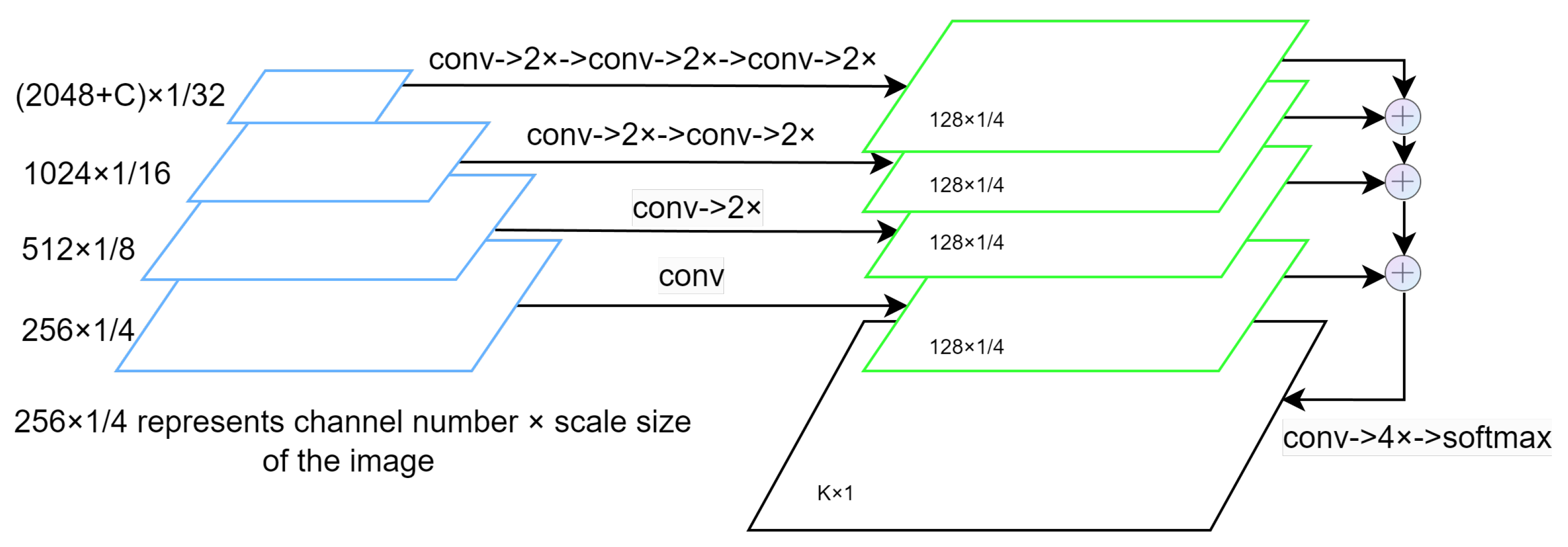
To obtain segmentation results from the fused and aligned image features and achieve text-guided segmentation prediction, this paper concatenates the extracted fourth layer image feature with the pixel–text score map by channel as the updated image feature. The multi-scale fusion strategy in Semantic FPN is used to upsample and fuse multi-scale image features, the specific fusion network is shown in Figure 3. Starting from the fourth feature layer, through convolutional layers and upsampling layers, the feature map is restored to 1/4 the size of the original image. Using the same strategy for each layer of feature maps, we obtain a set of feature maps with the same number of channels and sizes and then sum them element-wise. Finally, the convolution, upsampling, and softmax operations are used to predict the category label of each pixel and obtain the segmentation prediction result.
The main segmentation loss between the predicted segmentation results and the real labels and computed as follows:
L m a i n s e g = C r o s s E n t r o p y ( y ^ , y )
where y ^ and y represent the predicted segmentation result and the real label. Combining the segmentation loss, auxiliary segmentation loss, and contrastive loss to obtain the total loss as follows:
L = L m a i n s e g + λ 1 L a u x i s e g + λ 2 L c o n
where λ 1 and λ 2 are the hyperparameters applied to adjust the loss weight. The model is trained by the weighted sum among different losses to improve the segmentation performance of the model. The selection of parameters will be further introduced in the ablation experiment.

4. Experiments and Discussion

4.1. Experimental Settings

4.1.1. Dataset

To verify the semantic segmentation performance of the proposed BEMSeg model on remote sensing images, this paper conducted experiments on the Potsdam dataset [36] (ISPRS Potsdam 2D Semantic Labeling Challenge dataset), the Vaihingen dataset [37] (ISPRS Vaihingen 2D Semantic Labeling Challenge dataset) and the LoveDA dataset [38]. Both Potsdam and Vaihingen datasets have six categories, namely impervious surface, building, low vegetation, tree, car, and clutter. The LoveDA dataset has seven categories, namely background, building, road, water, barren, forest, and agricultural.
  • The Potsdam dataset contains 38 images with a spatial resolution of 5 cm and spectrum RGB. The image size is 6000 × 6000 pixels, taking the number of 2–10~2–12, 3–10~3–12, 4–10~4–12, 5–10~5–12, 6–7~6–12, and 7–7~7–12, a total of 24 images with ground truth labels as the training set, and the remaining 14 images are used as the test set.
  • The Vaihingen dataset contains 33 images with a spatial resolution of 9 cm and spectrum IRRG, the image size is not fixed, with an average of 2494 × 2064 pixels. Taking the number of areas, i.e., 1, 3, 5, 7, 11, 13, 15, 17, 21, 23, 26, 28, 30, 32, 34, and 37, a total of 16 images with ground truth labels as the training set, and the remaining 17 images are used as the test set.
  • The LoveDA dataset contains 5987 images that have been cropped into patches with 1024 × 1024 pixels. Following the official dataset split, 2522 images are used for training and 1669 images for test in the experiments.
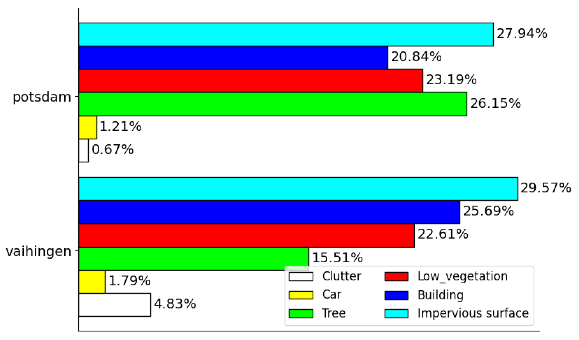
All images in the Potsdam and Vaihingen datasets are cropped into 512 × 512 pixels for model training. The proportion of pixels of each category in the total number of pixels in the two datasets is shown in Figure 4. It can be seen that the two datasets have the characteristics of class imbalance, for example, in the Vaihingen dataset, only the “clutter” and “car” category pixels account for 0.67% and 1.21% of the dataset, which are significantly lower than other categories.

4.1.2. Evaluation Metrics

Commonly used metrics in the field of image semantic segmentation are adopted for evaluation, including intersection over union (IoU), mean intersection over union (mIoU) and overall accuracy (OA). Among them, the IoU is used to compute the intersection and union ratio of the two sets of real labels and predicted values of a specific category, the mIoU represents the average of the IoU values for all categories. OA represents the ratio of correctly predicted pixels to all pixels which can evaluate the model’s accuracy and segmentation capabilities for all pixels. These evaluation metrics are computed as follows:
IoU c = n c , j j = 1 C n c , j + j = 1 C n j , c n c , c
mIoU = 1 C c = 1 C I o U c
OA = c = 1 C n c , c c = 1 C T c
where n c , c represents the number of pixels that belong to a class c and are correctly predicted as the class c, n j , c represents the number of pixels that belong to a class j but are incorrectly predicted as another class c, and C represents the total number of classes. T c represents the total number of pixels in the class c.

4.1.3. Implementation Details

The experimental equipment in this paper is Ubuntu 20.04.4 LTS, with a CPU of Intel®Xeon®Gold5215, and a GPU of GeForce RTX 3090 with 24 GB of memory. The model running environment is PyTorch1.10, Python3.8, CUDA11.4, using the AdanW [39] optimizer, weight decay is set to 0.0001, and the initial learning rate is set to 0.0001. To better maintain the pretraining weights, the text encoder parameters are frozen, and the learning rate coefficient in the image encoder is set to 0.1. The poly-learning strategy is adopted, the minimum learning rate is 1 × 10 6 , the training count uses the number of iterations, the data sent to a batch is trained for one iteration, the maximum number of iterations is 8 × 10 4 , and the batch size is set to 4. To understand the effect of different scales in images on segmentation performance, multi-scale testing (MS) is employed in the test stage.

4.2. Comparative Experiments and Analysis

BEMSeg model was compared with some classic and latest semantic segmentation methods including PSPNet [40], DeepLabV3+ [41], Semantic FPN [33], BANet [42], SwinB-CNN [43], GLOTS [44], HAFNet [45], CLIP–FPN, DenseCLIP [13] and LSeg [15]. CLIP-FPN is a basic multimodal segmentation method that is implemented in this paper. Table 1 and Table 2 list the network structure of comparison methods. The single-modal methods with the backbone of ResNet50 employ ResNetV1c (https://github.com/open-mmlab/mmpretrain/tree/main/configs/resnet, accessed on 1 June 2023) pretraining on the ImageNet as initialized weight, and the multimodal methods use the ResNet50 model and Transformer-based structure with pretraining CLIP weights (https://github.com/OpenAI/CLIP, accessed on 1 June 2023). The code will be available at https://github.com/liualice123/BEMSeg, accessed on 18 June 2024. All methods are trained and evaluated based on the same training and test sets.
A quantitative evaluation of the BEMSeg model and comparison methods was conducted on the Potsdam, Vaihingen, and LoveDA remote sensing datasets. The results are shown in Table 3, and the best results for each column are highlighted in bold. An analysis of the experimental results on the Potsdam dataset reveals the following: firstly, among the single-modal image semantic segmentation methods, the mIoU and OA values of the DeepLabV3+ network are 77.23% and 90.33% respectively, superior to the PSPNet, Semantic FPN, BANet, SwinB-CNN, GLOTS, and CLIP-FPN. DeepLabV3+ uses dilated convolution to expand the receptive field, however, the dilated spatial pyramid pooling operation increases the computational complexity of the model. HAFNet is an outstanding segmentation method specific for remote sensing images, which fully leverages the strengths of a Transformer-based decoder, channel adaptive module, global cross-fusion module, and other designs to achieve efficient performance.
Secondly, among the multimodal semantic segmentation methods, compared with the Semantic FPN model, the mIoU and OA results of the CLIP-FPN model on the Potsdam dataset improved by 0.18% and 0.36%. Although CLIP-FPN incorporates the alignment of image and text features, the guiding effect of text features on the image semantic segmentation task is not significant. The DenseCLIP model has a better performance than the CLIP-FPN model, the mIoU and OA improved by 1.41% and 0.41% on the Potsdam dataset. This indicates that the fusion of image context features into text features improves the model’s performance. Compared to DenseCLIP, the mIoU of BEMSeg improved by 2.02% on the Potsdam dataset, and the computation power only increased by 2.00%. This indicates the effectiveness of the proposed model in improving the accuracy of semantic segmentation for remote sensing images. The mIoU and OA values of LSeg are lower than BEMSeg by 1.09 and 0.69. BEMSeg shows the best segmentation performance on the Potsdam dataset with the mIoU surpassing comparison methods by 0.57% to 5.59% and with an OA improvement of 0.69% to 3.08%. The OA indicator is calculated as the proportion of correctly classified pixels to all pixels, due to the class imbalance problem in the Potsdam dataset, the difference in pixel numbers between “large classes” and “small classes” leads to a less obvious improvement in OA. The mIoU value of HAFNet is higher than that of LSeg while the OA value of HAFNet is lower than that of LSeg. This suggests that HAFNet primarily enhances the performance of the categories with fewer pixels, whereas LSeg mainly improves the performance of the categories with more pixels. The above conclusions are tenable on the Vaihingen dataset. On the LoveDA dataset, the mIoU and OA values of BEMSeg are lower than LSeg by 1.05 and 0.26. The LoveDA dataset has a complex background and more categories than Potsdam and Vaihingen, and Transformer-based methods such as GLOTS and LSeg can extract image features more accurately. Despite BEMSeg using CNN-based ResNet50 for feature extraction, with multimodal effective fusion and alignment, it still achieves a competitive performance. Table 3 also records the parameter quantity (params/M), computational complexity (GFLOPs), training time (/hours), and inference time (Frames Per Second, FPS) to evaluate the computational power and scale of the model. Because of the SPP/ASPP in PSPNet and DeepLabV3+, the Transformer-based encoding structure in SwinB-CNN, and Transformer-based decoder designs in HAFNet, the GFLOPS of these four methods are large. The parameters in the Transformer encoder of SwinB-CNN and GLOTS are more than those of CNN-based networks, and they also require more training time and process less image FPS in inference time. Compared with Semantic FPN and BANet, the multimodal semantic segmentation models incorporate a frozen Transformer-based text feature encoder, the increase in GFLOPs and parameters is not very large. BEMSeg adopts two cross-attention modules and contrastive learning to realize bidirectional feature fusion and enhance multimodal feature alignment, thus its parameters and training time are more than those of DenseCLIP. LSeg uses ViT-L to encode image features and performs multimodal feature alignment on the fused feature map with high resolution and more channels, which requires more training time and a large number of GFLOPs and parameters.
Regarding the segmentation performance of specific categories, the mIoU values of comparison methods on the Potsdam dataset are presented in Table 4. From the results in Table 4, the proposed BEMSeg achieves the best IoU values in all categories, significantly outperforming the other CNN and Transformer methods. DeepLabV3+ achieves a high IoU value of 41.48% on the clutter category, indicating that the ASPP operation is effective for categories with cluttered backgrounds. Semantic FPN uses multilayer image feature fusion and has better segmentation results for the car category with an IoU of 91.45%. HAFNet utilizes its global cross-fusion module and channel-spatial Transformer block in the decoder to aggregate global and local details, which improves its segmentation results for car and clutter categories, and the IoU values are 94.58% and 42.12%. In the multimodal comparison methods, LSeg performs feature alignment on the high-resolution feature map after simple feature fusion and uses depthwise convolution to obtain segmentation results, whereas BEMSeg performs multimodal alignment on high-level semantic features, and then combines multimodal alignment features and image features to obtain segmentation results by Semantic FPN. The results on LSeg and BEMSeg indicate that the multimodal feature alignment of high-level semantic image features with text features is probably more effective. Compared with DenseCLIP, the BEMSeg model improved the IoU of each category in the Potsdam dataset by 0.95%, 0.73%, 2.36%, 1.32%, 0.82%, and 7.75%, achieved larger improvements for the “clutter”, “tree” and “low vegetation” categories, and also improved the small object “car”. This indicates that the BEMSeg model can effectively improve the semantic segmentation performance of remote sensing images and mitigate the existing class imbalance problem.
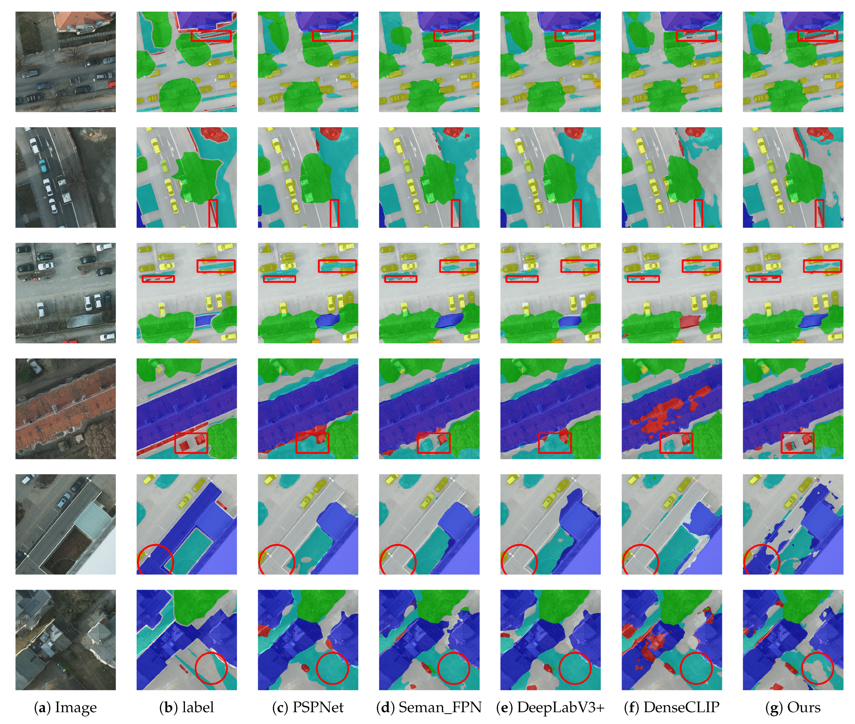
Figure 5 shows the qualitative semantic segmentation results of comparison methods on several test images of the Potsdam dataset. It can be seen that the BEMSeg model has achieved good semantic continuity in the “imperious surface” and “building” categories, and the segmentation map is relatively complete. For the “clutter” category with a relatively low proportion of pixel numbers, BEMSeg has also found the location of the categories and performed good segmentation. Compared with the comparison methods, the BEMSeg model has generally achieved superior segmentation results.
From Figure 6, it can be seen intuitively that the proposed BEMSeg method achieves the highest or second-highest IoU value for all categories of the Vaihingen dataset. As classical semantic segmentation methods, Semantic FPN performs well in the car category and DeepLabV3+ performs well in the clutter category. The performance of remote sensing semantic segmentation methods such as BANet, SwinB-CNN, and GLOTS on the Vaihingen dataset is poor, probably because the Transformer-based encoder cannot fully capture all the information on the few training images. HAFNet achieves the best IoU value in clutter by combining various global and local detailed features.
The LoveDA dataset has complex background samples and inconsistent class distributions, making it more challenging for accurate segmentation. The segmentation results of comparison methods on the LoveDA dataset are shown in Table 5, it can be seen that the performance of SwinB-CNN, GLOTS, and LSeg is superior to other CNN-based methods, mainly reflected in the “road”, “water” and “agriculture” categories, and LSeg obtains the best results on mIoU. This is probably because the Transformer-based encoder is more effective at capturing more complex and variable background samples on more training images. BEMSeg utilizes bidirectional feature fusion and alignment between text and image and achieves promising results on the “background”, “barren” and “forest” categories of the LoveDA dataset. Compared with Transformer-based methods, despite being based on CNN networks, BEMSeg still performs competitively on the LoveDA dataset.

4.3. Ablation Experiments

The role of different components in the BEMSeg model is demonstrated through ablation experiments. The network structure of CLIP-FPN is used as the baseline model, and the BFF module and the CPC learning are successively introduced into the model. The model with the BFF is referred to as BEMSeg-B, and the model with the CPC is referred to as BEMSeg-C. Table 6 and Table 7 record the experimental results of the model after adding different components to the Potsdam and Vaihingen datasets.
As shown in Table 6, the introduction of each component has improved the performance of the baseline model. Compared to the baseline model, the BEMSeg-B and BEMSeg-C models have improved all evaluation metric values in all categories, effectively mitigating the large intra-class variance and small inter-class variance problem of remote sensing images. The BEMSeg model obtained by combining the BBF module and CPC learning has improved the values of mIoU and OA by 3.43% and 1.36% on the Potsdam dataset, indicating that the combination of the two components is the best for improving the performance of semantic segmentation for remote sensing images. From the training time (/hours) and inference time (/FPS) of the model, the training times required for the baseline, BEMSeg-B, BEMSeg-C, and BEMSeg on the Potsdam dataset are 10.2 h, 12.0 h, 14.5 h, and 15.5 h, respectively. Compared with the baseline model, due to the addition of a cross-attention network and comparison learning, it inevitably increases the computation time of BEMSeg-B and BEMSeg-C. Additionally, because CPC learning is only used in the training phase, it does not increase the inference time of the model.
Regarding the segmentation performance of specific categories, compared with the baseline model, the IoU values of BEMSeg-C in each category have increased by 0.74%, 0.71%, 1.33%, 0.16%, 0.99% and 12.25%, and the IoU values of BEMSeg-B in each category have increased by 1.30%, 1.60%, 2.65%, 1.16%, 0.64% and 10.56%. For the “small class” like “car” and “clutter” in the imbalanced categories, the segmentation performance of the BEMSeg-C model that enhances the alignment of multimodal features through contrastive learning is more improved than BEMSeg-B. For the “imperious surface” and “low vegetation” categories in the “large class”, the segmentation performance of the BEMSeg-B model that uses a bidirectional fusion of multimodal features is more improved than BEMSeg-C. This indicates that based on improvements for all categories, BEMSeg-C is better for improving the segmentation performance of poor and small objects, and the category-based pixel-level contrastive loss plays a role in the phenomenon of class imbalance in remote sensing images; BEMSeg-B has a more prominent effect on the improvement of categories with a wide range and a large area, which is beneficial to alleviate the “same object with different spectra, different objects with similar spectra” problem in remote sensing images.
In Table 7, one can see that the BEMSeg model obtained by combining the BBF module and CPC learning has improved the values of mIoU and OA by 2.07% and 0.81% on the Vaihingen dataset. it can be concluded that in the “car” and “clutter” classes in the Vaihingen dataset, the segmentation performance of the BEMSeg-C model is more improved than BEMSeg-B. In the “imperious surface” and “low vegetation” categories, the segmentation performance of the BEMSeg-B model is more improved than BEMSeg-C, verifying the above conclusion on the Potsdam dataset.
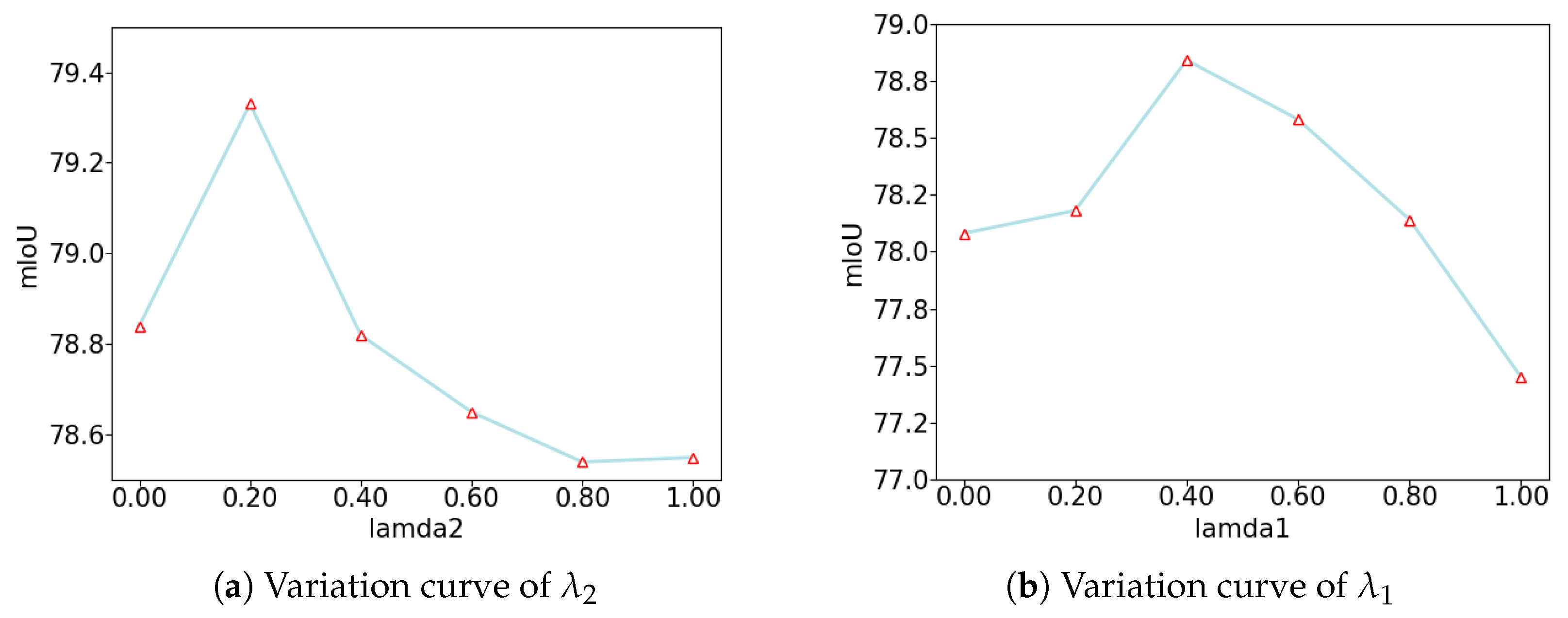
In the parameters setting of the loss function, the segmentation loss in the feature decoding process is the main loss, with a weight value of 1, λ 1 and λ 2 are used to control the weight of auxiliary segmentation loss and contrastive loss in the total loss, respectively, with the setting range of [0, 1]. Firstly refer to the [13] set λ 1 = 0.4 , update the value of λ 2 , and compare the results through experiments on the Potsdam dataset. Then select the best value of λ 2 from the experimental results, adjust the value of λ 1 , and compare the results through experiments. The mIoU results of the two-parameter variation experiments are shown in Figure 7.
As can be seen from Figure 7, when setting λ 1 = 0.4 , as λ 2 gradually increases, the performance of the BEMSeg model gradually improves, the mIoU reaches its best value of 79.33% when λ 2 = 0.2 , and then the model performance slightly declines. When setting λ 2 = 0.2 , the mIoU of the BEMSeg model gradually increases first and then decreases as the value of λ 1 increases. The mIoU reaches its best value of 78.84% when λ 1 = 0.4 . It can be concluded that when λ 1 = 0.4 ,   λ 2 = 0.2 , the total loss value combining contrastive loss and auxiliary segmentation loss plays the most significant role in improving the performance of the BEMSeg model. Although the auxiliary segmentation loss is computed under the supervision of real labels, due to its low resolution, it is easy to ignore detailed information during the upsampling process. The contrastive loss is obtained from the results on the pixel–text score map and it is easily affected by the error prediction of certain pixels when its loss value is too large, leading to a decline in model performance.

5. Conclusions

This paper proposes a new semantic segmentation model, BEMSeg, which utilizes both image and text multimodal information to address the challenges present in remote sensing images, such as “same object with different spectra, different objects with similar spectra”, large intra-class variance, small inter-class variance, and class imbalance. Experiments on the Potsdam, Vaihingen, and LoveDA datasets have demonstrated the superiorities of BEMSeg: firstly, it proposes a bidirectional feature fusion module to integrate image context features into text features and utilize text features to guide image feature representation. This module enhances the similarity of image features belonging to the same ground object, amplifies the difference among the image features of different ground objects, and facilitates the fusion of multimodal features. Secondly, on the pixel–text aligned score map, BEMSeg proposes a category-based pixel-level contrastive learning to close the distance between pixels of the same category, increase the distance between pixels of different categories, and enhance the alignment effect of image and text features. In addition, BEMSeg implements a positive and negative sample selection strategy based on different images for contrastive learning on the entire training dataset, further improving the model’s segmentation performance on imbalance categories like small objects and complex backgrounds. BEMSeg combines image and text multimodal information to achieve semantic segmentation for remote sensing images. Considering that text information can provide more prior knowledge, determining how to combine text to achieve domain adaptation and domain generalization of remote sensing images is the next research direction of this paper.

Author Contributions

Conceptualization, Q.L. and X.W.; methodology, Q.L. and X.W.; software, Q.L.; validation, Q.L. and X.W.; formal analysis, X.W.; writing—original draft preparation, Q.L.; writing—review and editing, Q.L. and X.W.; supervision, X.W.; funding acquisition, X.W. All authors have read and agreed to the published version of the manuscript.

Funding

This research was funded by the Second Tibetan Plateau Scientific Expedition and Research under grant no. 2019QZKK0405 and the National Natural Science Foundation of China under grant no. 42361056.

Data Availability Statement

The data in this paper can be obtained through the following links; ISPRS Potsdam: https://www.isprs.org/education/benchmarks/UrbanSemLab/2d-sem-label-potsdam.aspx, accessed on 1 June 2023; ISPRS Vaihingen: https://www.isprs.org/education/benchmarks/UrbanSemLab/2d-sem-label-vaihingen.aspx, accessed on 1 June 2023; The code will be available at https://github.com/liualice123/BEMSeg, accessed on 18 June 2024.

Conflicts of Interest

The authors declare no conflicts of interest.

Abbreviations

The following abbreviations are used in this manuscript:
VLPvision-language pretraining
NLPnatural language processing
MFTmultimodality fusion technology
BEMSegbidirectional feature fusion and enhanced alignment-based multimodal semantic segmentation
BFFbidirectional feature fusion
CPCcategory-based pixel-level contrastive
MSmulti-scale
SOTAstate-of-the-art

References

  1. Marcos, D.; Volpi, M.; Kellenberger, B.; Tuia, D. Land cover mapping at very high resolution with rotation equivariant CNNs: Towards small yet accurate models. ISPRS J. Photogramm. Remote Sens. 2018, 145, 96–107. [Google Scholar] [CrossRef]
  2. Qin, P.; Cai, Y.; Liu, J.; Fan, P.; Sun, M. Multilayer feature extraction network for military ship detection from high-resolution optical remote sensing images. IEEE J. Sel. Top. Appl. Earth Obs. Remote Sens. 2021, 14, 11058–11069. [Google Scholar] [CrossRef]
  3. Tang, X.; Tu, Z.; Wang, Y.; Liu, M.; Li, D.; Fan, X. Automatic detection of coseismic landslides using a new transformer method. Remote Sens. 2022, 14, 2884. [Google Scholar] [CrossRef]
  4. Wang, P.; Tang, Y.; Liao, Z.; Yan, Y.; Dai, L.; Liu, S.; Jiang, T. Road-side individual tree segmentation from urban MLS point clouds using metric learning. Remote Sens. 2023, 15, 1992. [Google Scholar] [CrossRef]
  5. Ronneberger, O.; Fischer, P.; Brox, T. U-net: Convolutional networks for biomedical image segmentation. In Proceedings of the International Conference on Medical Image Computing and Computer-Assisted Intervention, Munich, Germany, 5–9 October 2015; pp. 234–241. [Google Scholar]
  6. Lin, T.Y.; Dollár, P.; Girshick, R.; He, K.; Hariharan, B.; Belongie, S. Feature pyramid networks for object detection. In Proceedings of the IEEE Conference on Computer Vision and Pattern Recognition, Honolulu, HI, USA, 21–26 July 2017; pp. 2117–2125. [Google Scholar]
  7. Chen, L.C.; Papandreou, G.; Schroff, F.; Adam, H. Rethinking atrous convolution for semantic image segmentation. arXiv 2017, arXiv:1706.05587. [Google Scholar]
  8. Zhao, H.; Zhang, Y.; Liu, S.; Shi, J.; Loy, C.C.; Lin, D.; Jia, J. Psanet: Point-wise spatial attention network for scene parsing. In Proceedings of the European Conference on Computer Vision (ECCV), Munich, Germany, 8–14 September 2018; pp. 267–283. [Google Scholar]
  9. Ranftl, R.; Bochkovskiy, A.; Koltun, V. Vision transformers for dense prediction. In Proceedings of the IEEE/CVF International Conference on Computer Vision, Montreal, BC, Canada, 11–17 October 2021; pp. 12179–12188. [Google Scholar]
  10. Liu, M.; Fan, J.; Liu, Q. Biomedical image segmentation algorithm based on dense atrous convolution. Math. Biosci. Eng. 2024, 21, 4351–4369. [Google Scholar] [CrossRef]
  11. Radford, A.; Kim, J.W.; Hallacy, C.; Ramesh, A.; Goh, G.; Agarwal, S.; Sastry, G.; Askell, A.; Mishkin, P.; Clark, J. Learning transferable visual models from natural language supervision. In Proceedings of the International Conference on Machine Learning, Virtual, 18–24 July 2021; pp. 8748–8763. [Google Scholar]
  12. Ghiasi, G.; Gu, X.; Cui, Y.; Lin, T.Y. Open-vocabulary image segmentation. arXiv 2021, arXiv:2112.12143. [Google Scholar]
  13. Rao, Y.; Zhao, W.; Chen, G.; Tang, Y.; Zhu, Z.; Huang, G.; Zhou, J.; Lu, J. Denseclip: Language-guided dense prediction with context-aware prompting. In Proceedings of the IEEE/CVF Conference on Computer Vision and Pattern Recognition, New Orleans, LA, USA, 18–24 June 2022; pp. 18082–18091. [Google Scholar]
  14. Kirillov, A.; Mintun, E.; Ravi, N.; Mao, H.; Rolland, C.; Gustafson, L.; Xiao, T.; Whitehead, S.; Berg, A.C.; Lo, W.Y. Segment anything. arXiv 2023, arXiv:2304.02643. [Google Scholar]
  15. Li, B.; Weinberger, K.Q.; Belongie, S.; Koltun, V.; Ranftl, R. Language-Driven Semantic Segmentation. In Proceedings of the ICLR 2022—10th International Conference on Learning Representations, Virtual, 25–29 April 2022. [Google Scholar]
  16. Xu, J.; De Mello, S.; Liu, S.; Byeon, W.; Breuel, T.; Kautz, J.; Wang, X. Groupvit: Semantic segmentation emerges from text supervision. In Proceedings of the IEEE/CVF Conference on Computer Vision and Pattern Recognition, New Orleans, LA, USA, 18–24 June 2022; pp. 18134–18144. [Google Scholar]
  17. Zhou, K.; Yang, J.; Loy, C.C.; Liu, Z. Learning to prompt for vision-language models. Int. J. Comput. Vis. 2022, 130, 2337–2348. [Google Scholar] [CrossRef]
  18. Lüddecke, T.; Ecker, A. Image segmentation using text and image prompts. In Proceedings of the IEEE/CVF Conference on Computer Vision and Pattern Recognition, New Orleans, LA, USA, 18–24 June 2022; pp. 7086–7096. [Google Scholar]
  19. Ramachandram, D.; Taylor, G.W. Deep multimodal learning: A survey on recent advances and trends. IEEE Signal Process. Mag. 2017, 34, 96–108. [Google Scholar] [CrossRef]
  20. Wei, X.; Zhang, T.; Li, Y.; Zhang, Y.; Wu, F. Multi-modality cross attention network for image and sentence matching. In Proceedings of the IEEE/CVF Conference on Computer Vision and Pattern Recognition, Seattle, WA, USA, 13–19 June 2020; pp. 10941–10950. [Google Scholar]
  21. Kato, N.; Yamasaki, T.; Aizawa, K. Zero-shot semantic segmentation via variational mapping. In Proceedings of the IEEE/CVF International Conference on Computer Vision Workshops, Seoul, Republic of Korea, 27–28 October 2019. [Google Scholar]
  22. Li, X.; Wen, C.; Hu, Y.; Zhou, N. Rs-clip: Zero shot remote sensing scene classification via contrastive vision-language supervision. Int. J. Appl. Earth Obs. Geoinf. 2023, 124, 103497. [Google Scholar] [CrossRef]
  23. Jia, C.; Yang, Y.; Xia, Y.; Chen, Y.T.; Parekh, Z.; Pham, H.; Le, Q.; Sung, Y.H.; Li, Z.; Duerig, T. Scaling up visual and vision-language representation learning with noisy text supervision. In Proceedings of the International Conference on Machine Learning, Virtual, 18–24 July 2021; pp. 4904–4916. [Google Scholar]
  24. Chen, J.; Zhu, D.; Qian, G.; Ghanem, B.; Yan, Z.; Zhu, C.; Xiao, F.; Culatana, S.C.; Elhoseiny, M. Exploring open-vocabulary semantic segmentation from clip vision encoder distillation only. In Proceedings of the IEEE/CVF International Conference on Computer Vision, Paris, France, 2–6 October 2023; pp. 699–710. [Google Scholar]
  25. Zhou, Z.; Lei, Y.; Zhang, B.; Liu, L.; Liu, Y. Zegclip: Towards adapting clip for zero-shot semantic segmentation. In Proceedings of the IEEE/CVF Conference on Computer Vision and Pattern Recognition, Vancouver, BC, Canada, 17–24 June 2023; pp. 11175–11185. [Google Scholar]
  26. Gao, P.; Geng, S.; Zhang, R.; Ma, T.; Fang, R.; Zhang, Y.; Li, H.; Qiao, Y. Clip-adapter: Better vision-language models with feature adapters. Int. J. Comput. Vis. 2024, 132, 581–595. [Google Scholar] [CrossRef]
  27. Baltrušaitis, T.; Ahuja, C.; Morency, L.P. Multimodal machine learning: A survey and taxonomy. IEEE Trans. Pattern Anal. Mach. Intell. 2018, 41, 423–443. [Google Scholar] [CrossRef] [PubMed]
  28. Guo, S.C.; Liu, S.K.; Wang, J.Y.; Zheng, W.M.; Jiang, C.Y. CLIP-Driven Prototype Network for Few-Shot Semantic Segmentation. Entropy 2023, 25, 1353. [Google Scholar] [CrossRef] [PubMed]
  29. Kiela, D.; Grave, E.; Joulin, A.; Mikolov, T. Efficient large-scale multi-modal classification. In Proceedings of the AAAI Conference on Artificial Intelligence, New Orleans, LA, USA, 2–7 February 2018; Volume 32. [Google Scholar]
  30. Vaswani, A.; Shazeer, N.; Parmar, N.; Uszkoreit, J.; Jones, L.; Gomez, A.N.; Kaiser, Ł.; Polosukhin, I. Attention is all you need. Adv. Neural Inf. Process. Syst. 2017, 30, 5998–6008. [Google Scholar]
  31. Xu, P.; Zhu, X.; Clifton, D.A. Multimodal learning with transformers: A survey. IEEE Trans. Pattern Anal. Mach. Intell. 2023, 45, 12113–12132. [Google Scholar] [CrossRef]
  32. Jiao, S.; Wei, Y.; Wang, Y.; Zhao, Y.; Shi, H. Learning mask-aware clip representations for zero-shot segmentation. Adv. Neural Inf. Process. Syst. 2023, 36, 35631–35653. [Google Scholar]
  33. Kirillov, A.; Girshick, R.; He, K.; Dollár, P. Panoptic feature pyramid networks. In Proceedings of the IEEE/CVF Conference on Computer Vision and Pattern Recognition, Long Beach, CA, USA, 15–20 June 2019; pp. 6399–6408. [Google Scholar]
  34. Lu, J.; Batra, D.; Parikh, D.; Lee, S. ViLBERT: Pretraining task-agnostic visiolinguistic representations for vision-and-language tasks. Adv. Neural Inf. Process. Syst. 2019, 32, 13–23. [Google Scholar]
  35. Wang, W.; Zhou, T.; Yu, F.; Dai, J.; Konukoglu, E.; Van Gool, L. Exploring cross-image pixel contrast for semantic segmentation. In Proceedings of the IEEE/CVF International Conference on Computer Vision, Montreal, BC, Canada, 11–17 October 2021; pp. 7303–7313. [Google Scholar]
  36. Potsdam. ISPRS Potsdam 2D Semantic Labeling Dataset, 2018. Available online: https://www.isprs.org/education/benchmarks/UrbanSemLab/2d-sem-label-potsdam.aspx (accessed on 1 June 2023).
  37. Vaihingen. ISPRS Vaihingen 2D Semantic Labeling Dataset, 2018. Available online: https://www.isprs.org/education/benchmarks/UrbanSemLab/2d-sem-label-vaihingen.aspx (accessed on 1 June 2023).
  38. Wang, J.; Zheng, Z.; Ma, A.; Lu, X.; Zhong, Y. LoveDA: A Remote Sensing Land-Cover Dataset for Domain Adaptive Semantic Segmentation. arXiv 2021, arXiv:2110.08733. [Google Scholar]
  39. Loshchilov, I.; Hutter, F. Decoupled weight decay regularization. arXiv 2017, arXiv:1711.05101. [Google Scholar]
  40. Zhao, H.; Shi, J.; Qi, X.; Wang, X.; Jia, J. Pyramid scene parsing network. In Proceedings of the IEEE Conference on Computer Vision and Pattern Recognition, Honolulu, HI, USA, 21–26 July 2017; pp. 2881–2890. [Google Scholar]
  41. Chen, L.C.; Zhu, Y.; Papandreou, G.; Schroff, F.; Adam, H. Encoder-decoder with atrous separable convolution for semantic image segmentation. In Proceedings of the European Conference on Computer Vision (ECCV), Munich, Germany, 8–14 September 2018; pp. 801–818. [Google Scholar]
  42. Wang, L.; Li, R.; Wang, D.; Duan, C.; Wang, T.; Meng, X. Transformer Meets Convolution: A Bilateral Awareness Network for Semantic Segmentation of Very Fine Resolution Urban Scene Images. Remote Sens. 2021, 13, 3065. [Google Scholar] [CrossRef]
  43. Zhang, C.; Jiang, W.; Zhang, Y.; Wang, W.; Zhao, Q.; Wang, C. Transformer and CNN hybrid deep neural network for semantic segmentation of very-high-resolution remote sensing imagery. IEEE Trans. Geosci. Remote Sens. 2022, 60, 1–20. [Google Scholar] [CrossRef]
  44. Liu, Y.; Zhang, Y.; Wang, Y.; Mei, S. Rethinking transformers for semantic segmentation of remote sensing images. IEEE Trans. Geosci. Remote Sens. 2023. [Google Scholar] [CrossRef]
  45. Chen, Y.; Dong, Q.; Wang, X.; Zhang, Q.; Kang, M.; Jiang, W.; Wang, M.; Xu, L.; Zhang, C. Hybrid Attention Fusion Embedded in Transformer for Remote Sensing Image Semantic Segmentation. IEEE J. Sel. Top. Appl. Earth Obs. Remote Sens. 2024, 17, 4421–4435. [Google Scholar] [CrossRef]
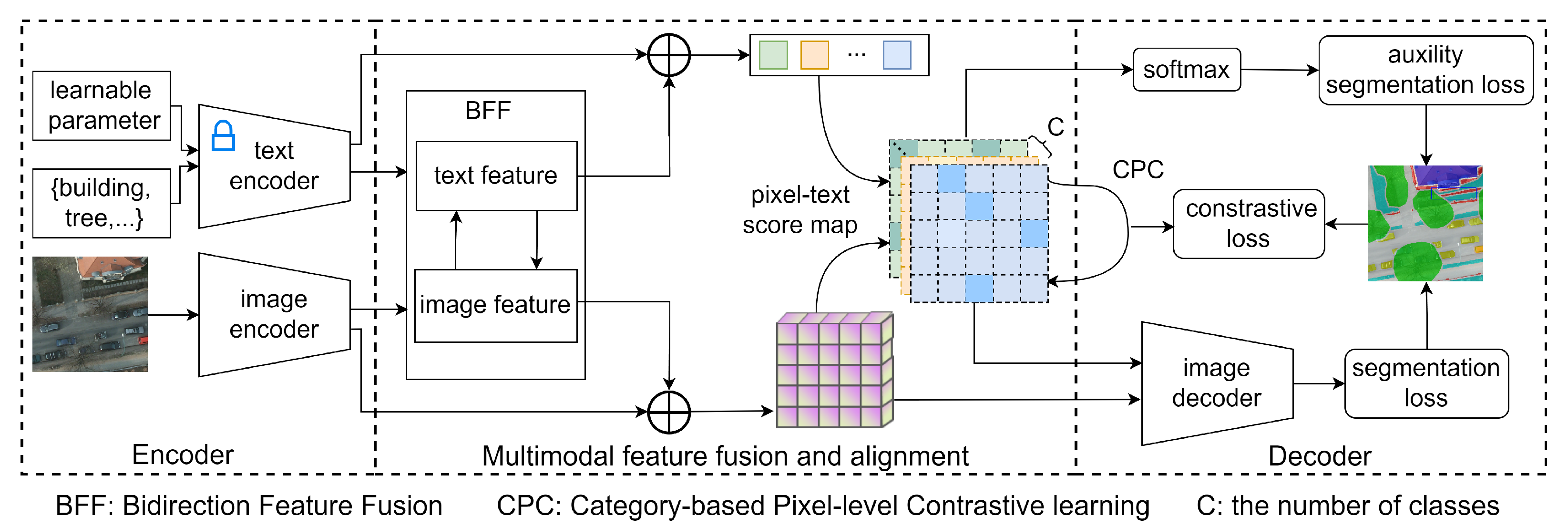
Figure 1. The framework of the proposed BEMSeg, which consists of an image encoder, a text encoder, multimodal feature fusion, an alignment module, and a decoder. BFF and CPC denote the bidirectional feature fusion module and category-based pixel-level contrastive learning in the multimodal feature fusion and alignment module, and C denotes the number of categories. The colored squares at the top denote the text features of different categories.
Remotesensing 16 02289 g001
Figure 2. We propose a new attention-based bidirectional feature fusion module. This structure enables image-attention text features to be incorporated into text representations (and vice versa) by designing a dual-branch structure and adding a self-attention mechanism.
Remotesensing 16 02289 g002
Figure 3. Multi-scale image feature fusion network in the decoder of Semantic FPN.
Remotesensing 16 02289 g003
Figure 4. Proportion of the number of pixels in each category in Potsdam and Vaihingen remote sensing datasets.
Remotesensing 16 02289 g004
Figure 5. The qualitative results of comparison methods on some test images of the Potsdam dataset.
Remotesensing 16 02289 g005
Figure 6. The IoU of each class of comparison methods on the Vaihingen dataset.
Remotesensing 16 02289 g006
Figure 7. Different parameters of λ 1 and λ 2 correspond to the mIoU value of the BEMSeg model on the Potsdam dataset.
Remotesensing 16 02289 g007
Table 1. Details of single-modal comparison methods.
MethodsBackboneSPP/ASPPTransformer EncoderSpatial/Channel AttentionTransformer DncoderMultilayer Feature Fusion
PSPNetResNet50
DeepLabV3+ResNet50
Semantic FPNResNet50
BANetResT-Lite
SwinB-CNNSwin Transformer
GLOTSVit-B
HAFNetResNet50
Table 2. Details of multimodal comparison methods.
MethodsBackboneImage FeatureText FeatureImage-to-Text FusionText-to-Image FusionMultimodal AlignmentContrastive Learning
CLIP-FPNResNet50
DenseCLIPResNet50
LSegViT-L
BEMSegResNet50
Table 3. The quantitative evaluation results of comparison methods and the complexities metrics are based on the Potsdam dataset, and the best result for each column is highlighted in bold.
MethodsPotsdamVaihingenLoveDAGFLOPsParams
/M
Training
Time/h
Inference
Time/FPS
mIoU/%OA/%mIoU/%OA/%mIoU/%OA/%
PSPNet76.6390.2570.3290.0547.4366.78201.5953.324.247.6
DeepLabV3+77.2390.3370.7990.1350.1868.65198.3352.044.542.2
Semantic FPN75.7289.5373.6789.9450.0168.6845.4028.504.542.1
BANet73.7488.1770.0188.09--58.1028.58--
SwinB-CNN75.1089.2168.7987.6554.2070.52114.00104.02-25.3
GLOTS76.0289.9670.1388.2455.6370.85---19.8
HAFNet78.7690.4576.3790.29--114.6438.51--
CLIP-FPN75.9089.8974.2190.1550.9968.8562.6031.0010.240.3
DenseCLIP77.3190.3074.6990.2852.1769.5069.3050.1711.736.6
LSeg78.2490.5675.8090.8755.7670.92--44.6-
BEMSeg79.3391.2576.2890.9654.7170.6670.3054.1215.534.0
Table 4. The IoU of each class of comparison methods on the Potsdam dataset, and the best result for each column is highlighted in bold.
MethodsImperious SurfaceBuildingLow VegetationTreeCarCluttermIoU/%
PSPNet86.1392.9776.0979.2987.8737.4576.63
DeepLabV3+86.0192.6676.4679.5087.3041.4877.23
Semantic FPN85.6992.6775.7179.0591.4529.7775.72
BANet83.3589.1473.5574.5687.9933.8873.74
SwinB-CNN84.5292.475.0776.8882.6639.0675.10
GLOTS85.2092.1975.2376.9784.3742.1576.02
HAFNet85.9492.5476.8979.3291.5842.1278.06
CLIP_FPN86.2692.4275.2579.0591.8130.5875.90
DenseCLIP86.7093.2675.8979.0591.5535.6277.31
LSeg87.1492.9976.4579.1591.1942.5578.24
BEMSeg87.6593.9978.2580.3792.3743.3779.33
Table 5. The IoU of each class of comparison methods on the LoveDA dataset, and the best result for each column is highlighted in bold.
MethodsBackgroundBuildingRoadWaterBarrenForestAgriculturemIoU/%
PSPNet52.7362.7551.3357.4823.0636.4348.2147.43
DeepLabV3+53.9863.8754.0562.0729.2438.5949.4550.18
Semantic FPN53.0562.7053.7067.3423.0842.0848.0150.01
SwinB-CNN53.6065.9858.3672.6731.6043.5653.6254.20
GLOTS55.2767.0659.6173.0829.1845.0660.0955.63
CLIP_FPN53.2864.8153.8465.2927.2643.8848.5350.99
DenseCLIP53.2963.9554.4467.5031.6444.0050.3452.17
LSeg55.5267.3259.7273.8632.4645.6355.7955.76
BEMSeg56.7967.0556.7770.4332.5245.7753.6554.71
Table 6. The results of ablation experiments on the Potsdam dataset, and the best result for each column is highlighted in bold.
MethodsIoU Per Class/%mIoU/%mF1/%OA/%Training
Time/h
Inference
Time/FPS
Imperious SurfaceBuildingLow VegetationTreeCarClutter
Baseline86.2692.4275.2579.0591.8130.5875.9084.2489.8910.240.3
BEMSeg-B87.5693.8277.9080.2192.4541.1478.8486.8891.1712.034.0
BEMSeg-C87.0093.1376.5879.2192.8042.8378.5986.1191.0114.540.3
BEMSeg87.6593.9978.2580.3792.8742.8779.3387.2991.2515.534.0
Table 7. The results of ablation experiments on the Vaihingen dataset, and the best result for each column is highlighted in bold.
MethodsIoU Per Class/%mIoU/%mF1/%OA/%
Imperious SurfaceBuildingLow VegetationTreeCarClutter
Baseline86.0091.6370.9179.7177.9839.0174.2183.9390.15
BEMSeg-B86.6892.0073.2481.3279.0241.8475.6885.0890.87
BEMSeg-C86.3691.7872.1380.9579.5642.8675.6085.1590.79
BEMSeg86.7892.0173.4281.4779.7344.2976.2885.5690.96
Disclaimer/Publisher’s Note: The statements, opinions and data contained in all publications are solely those of the individual author(s) and contributor(s) and not of MDPI and/or the editor(s). MDPI and/or the editor(s) disclaim responsibility for any injury to people or property resulting from any ideas, methods, instructions or products referred to in the content.