Article

Algorithms for Hyperparameter Tuning of LSTMs for Time Series Forecasting

by
Harshal Dhake
1,
Yashwant Kashyap
1,* and
Panagiotis Kosmopoulos
2,*
1
Department of Electrical and Electronics Engineering, National Institute of Technology Karnataka, Surathkal 575025, India
2
Institute for Environmental Research and Sustainable Development, National Observatory of Athens (IERSD/NOA), 15236 Athens, Greece
*
Authors to whom correspondence should be addressed.
Remote Sens. 2023, 15(8), 2076; https://doi.org/10.3390/rs15082076
Submission received: 17 February 2023 / Revised: 8 April 2023 / Accepted: 12 April 2023 / Published: 14 April 2023
(This article belongs to the Section Urban Remote Sensing)

Abstract

:
The rapid growth in the use of Solar Energy for sustaining energy demand around the world requires accurate forecasts of Solar Irradiance to estimate the contribution of solar power to the power grid. Accurate forecasts for higher time horizons help to balance the power grid effectively and efficiently. Traditional forecasting techniques rely on physical weather parameters and complex mathematical models. However, these techniques are time-consuming and produce accurate results only for short forecast horizons. Deep Learning Techniques like Long Short Term Memory (LSTM) networks are employed to learn and predict complex varying time series data. However, LSTM networks are susceptible to poor performance due to improper configuration of hyperparameters. This work introduces two new algorithms for hyperparameter tuning of LSTM networks and a Fast Fourier Transform (FFT) based data decomposition technique. This work also proposes an optimised workflow for training LSTM networks based on the above techniques. The results show a significant fitness increase from 81.20% to 95.23% and a 53.42% reduction in RMSE for 90 min ahead forecast after using the optimised training workflow. The results were compared to several other techniques for forecasting solar energy for multiple forecast horizons.

1. Introduction

Over recent years, the focus has shifted to exploiting sustainable sources of energy. Forecasting Solar Irradiance several timesteps ahead can prove beneficial to power stations in grid management and conventional-non-conventional energy balance in the grid [1]. Machine Learning (ML), Neural Networks (NNs) and Stochastic Models like Autoregressive Integrated Moving Average (ARIMA) Models have been applied to learn and understand the patterns of variations in Solar Irradiance to forecast the production of Solar Energy. There are 4 commonly used techniques for Solar Energy forecasting, Statistical, Physical, ML-based and Artificial Intelligence (AI) based methods according to Wang et al., 2018 [2]. Physical Models are deterministic models which use lower atmospheric parameters to understand the data and its patterns before making the forecast. Thus the physical methods are more complex, time-consuming and less accurate for long-term forecasts. Statistical Methods use mathematical models to forecast and have been widely used for time series forecasting [3]. These models may be linear or non-linear but give good performance only for short-duration forecasts [4,5]. Colak et al., 2015 [6] employed the ARIMA model for forecasting Solar Radiation for up to 3 h ahead and obtained a mean absolute percentage error of 92.37%. The Seasonal ARIMA (SARIMA) model was used to forecast monthly average insolation around the regions of Delhi, India, obtaining an R 2 score of 92.93% in Shadab et al., 2020 [7]. It was observed that ML and AI methods produce good long-term forecasting results compared to statistical and physical methods, despite having no clear understanding of the data [8].
NNs perform better than traditional ML forecasting algorithms and techniques like ARIMA for time series forecasting [9,10]. Recurrent Neural Networks (RNNs) were used initially for forecasting but RNNs are unable to learn the relevant information from input data when the input gap is large. Long Short Term Memory (LSTMs) can handle long-term dependencies due to its gate functions [11]. LSTMs form a neural network with the nodes unwrapped over time and allow the network to take advantage of previous calculations. LSTM is used to forecast Solar Energy due to its intermittent nature [12,13].
LSTM Networks are highly configurable through several hyperparameters. Choosing the correct set of hyperparameters for the network is crucial because it directly impacts the model’s performance. According to Bischl et al., 2021 [14], the brute force search for hyperparameters is time-consuming and irreproducible for different runs of the model. This highly unreliable trial-and-error technique slows the entire machine-learning process pipeline. Falkner et al., 2018 [15] explore several techniques like Bayesian optimisation and bandit-based methods in the domain of hyperparameter tuning providing a practical solution for several desired statistics in ML models like Strong Anytime Performance, Strong Final Performance, Effective use of parallel resources, scalability, robustness and flexibility. Hyperparameter Tuning is the process of finding the optimal set of hyperparameters which generate a network with maximum performance. Hyperparameter Tuning and Feature Selection should be used alongside as it helps in minimising the ratio of resources allocated to the performance obtained from the model [16]. Hyperparameter Tuning algorithms usually work on balancing the following two factors which affect the optimisation power of the algorithm:
  • Trade-off between the exploration and exploitation of the search space of hyperparameters. This affects the bias of the algorithm to perform a local search near the current best-selected search agents or perform a random search to attain a new set of search agents. Such trade-offs are generally affected by resource constraints.
  • Trade-off between inference and search of hyperparameters. The algorithm generates a new set of hyperparameters from the currently available set of hyperparameters either by searching for better hyperparameters or inferencing from the existing set. This refers to the exploitation characteristic of the algorithm.
The Genetic Algorithm is an optimisation algorithm based on the evolution principle found in nature. The algorithm consists of 6 fundamental steps, Population Initialisation, Fitness Evaluation, Termination Condition check, Random Selection, Breeding or Crossover, and Random Mutation. Population Initialisation is responsible for generating the initial population which has to be optimised. Fitness Evaluation finds out the fitness of each member of the population using the objective or the fitness function. This fitness value helps in obtaining the best member out of the population. The Random Selection step ensures that two unique members are chosen randomly (following a uniform random distribution pattern) for breeding. The Breeding or Crossover step is responsible for generating children from the randomly chosen parent members. These children may randomly mutate in the Random Mutation step and are added to the population thereafter. Finally, the algorithm terminates if the number of generations exceeds the specified value or any termination condition mentioned has been satisfied [17]. Gorgolis et al., 2019 [17] also explores the use of the Genetic Algorithm for tuning the hyperparameters for LSTM Network Models and uses an n-dimensional configuration spacefor hyperparameter optimisation where n is the number of configurable hyperparameters of the network. LSTMs are highly sensitive towards network parameters like the number of hidden layers, number of cell units in each layer, activation functions, size of history time input and so on, which drastically affect the model’s performance. Genetic Algorithm based optimiser has also been explored in several other time-series forecasting problems (like stock market prediction) using LSTMs and has given out good results [18].
Heap Based Optimiser (HBO) has been used extensively for Feature Selection for Time Series Applications using LSTMs [19] and for extraction of parameters of various models [20,21] while works like Ginidi et al., 2021 [22] use HBO to solve complex optimisation problems. HBO uses a heap data structure to organise the input data population and applies the Corporate Ranking Hierarchy (CRH) to it. CRH ensures that the algorithm does not get stuck on local optima, which is a common problem faced by several optimisation algorithms [23].
This paper makes the following contributions:
  • Decomposing Time Series Data using Fast Fourier Transform to extract logical and meaningful information from the raw data.
  • Two algorithms and an optimized workflow for tuning hyperparameters of LSTM networks using HBO and GA have been designed and developed for potential operational-ready applications.
  • The effect of two different optimizers on LSTM Networks and the effect of data decomposition on the network’s forecast performance and efficiency have been analyzed and inter-compared.
  • The optimized LSTM Network with the default network using 90 min ahead forecast has been evaluated and compared. The impact and the necessity of hyperparameter tuning are highlighted and depicted through the comparisons performed.
The rest of the paper is structured as follows. Section 2.1 describes the data processing involved in the system, which contains feature selection, data scaling and supervised time series conversion in Section 2.1.1 and Section 2.1.2 and the data decomposition in Section 2.1.3. Section 2.2 describes the Optimiser Design for Hyperparameter Tuning, which consists of Section 2.2.1 elucidating HBO and Section 2.2.2 describing Genetic Algorithm Based Optimiser (GAO). The results and observations are presented in Section 3. Conclusions are presented in Section 4.

2. Methodology

2.1. Data Processing

This paper used raw data similar to data used in Kumar et al., 2022 [24]. The collected raw data contained 154,277 entries of solar irradiance (W m−2) received from 22 different locations of a solar power plant in Southern India and the net irradiance received. The raw data was timestamped with each record at an interval of 5 min. Each of the 22 inputs is labelled as a feature and the net irradiance is labelled as output. The desired output of the forecast was the 18th point from the current i.e., 90 min ahead forecast. The raw data was further processed as described in the following sections.

2.1.1. Feature Selection and Data Processing

Feature Selection is done after plotting each of these features individually and in a correlation matrix to understand their influence on the data and their relationships with the target variable as well as with other variables. The data contained input features which were highly correlated with the output as well as with each other. Hence, all of the features were selected to minimise the loss of information after feature selection. To avoid bias towards the features having higher numerical values, each of the features was scaled to the range [ 0 ,   1 ] . This scaling is applied to the input as well as the output to maintain the original relation between them. This scaling is inverted after the forecasting process to obtain the actual value of the output instead of the normalised value. Also, the NULL values were filled with the average value of the feature to avoid deviancy in data and retain the feature correlation with others. Figure 1 shows the correlation matrix obtained for the raw data.

2.1.2. Conversion to Supervised Time Series

LSTM network requires data in a supervised time series format. A supervised data set implies that the input features and the output variable have to be separated. A time series implies that data must form a series with its terms separated over time. The output variable is assumed to be influenced by previous data of all the input features as well as the previous values of the output variable itself. The steps followed to convert the data to supervised time series are as follows,
1.
Column Axis Shifting to generate Time Series:
All the input features were shifted by 18 to 1 records on the column axis to create a time series of length 18 points as follows,
f e a t u r e ( t 18 ) , f e a t u r e ( t 17 ) , f e a t u r e ( t 16 ) . . . . . . f e a t u r e ( t 1 )
The past value of the output variable is also considered as an input feature and forms the input pattern similar to one observed in Jursa and Rohrig, 2008 [25]. The output variable is shifted forward by 18 points i.e., o u t p u t ( t + 18 ) is the actual time series output which is to be forecasted.
2.
Reshaping the Data for LSTM Network:
After creating the time series, the data consisted of 18 × 23 = 414 input features and 1 output column. The input vector is a two-dimensional vector and is not compatible with LSTM networks. The input data needs to be reshaped as,
[ s a m p l e s , t i m e s t e p s , f e a t u r e s ]
Hence the input vector is reshaped into a three-dimensional vector,
[ 154258 , 18 , 23 ]

2.1.3. Data Decomposition

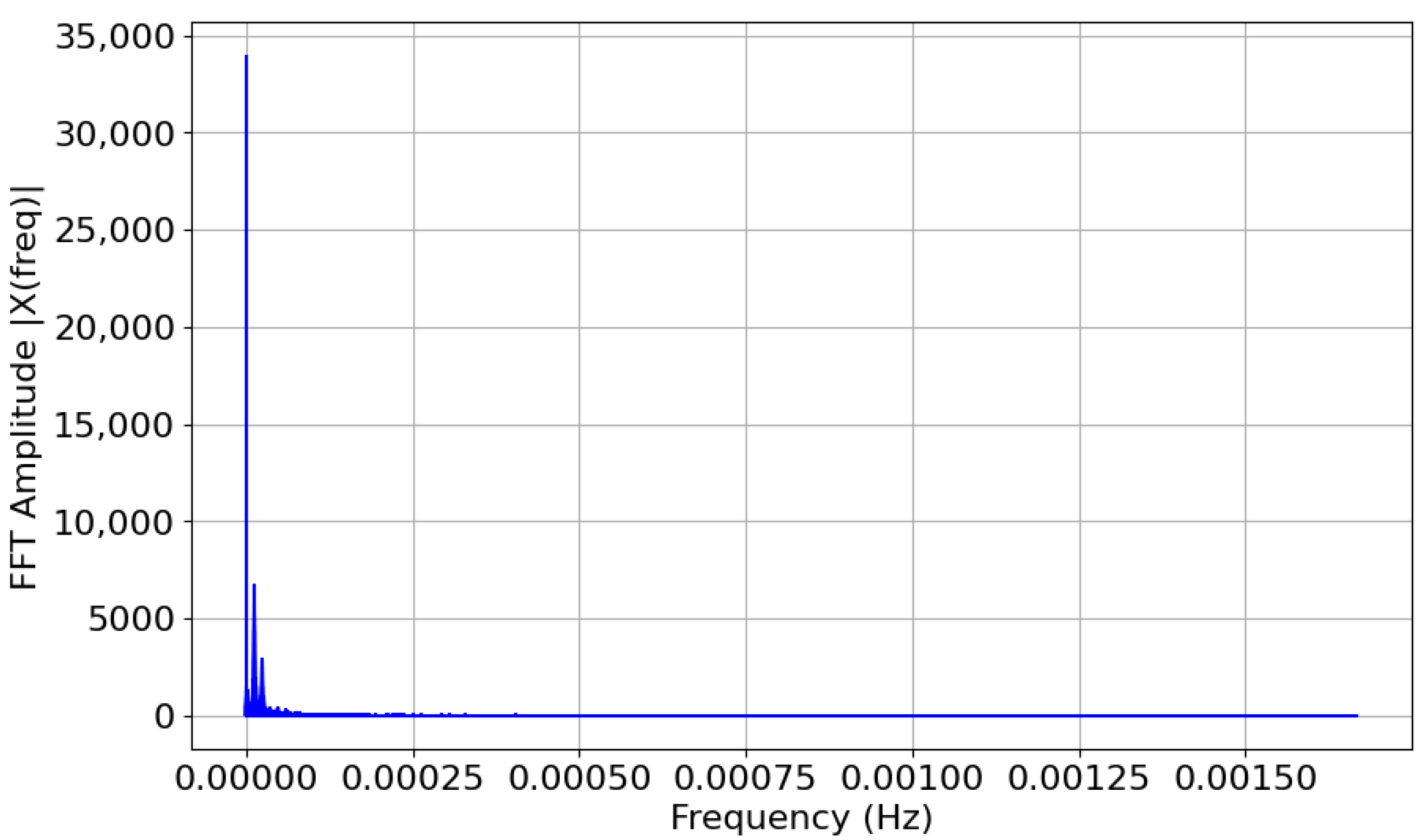
The data was decomposed into two components: High Frequency (HF) Data and Low Frequency (LF) data, using the Fourier Transform to extract long-term trends and other information which would aid the LSTM network for forecasting. The data was analysed using the Fast Fourier Transform technique [26] to obtain an optimal decomposition. FFT is an efficient approach to calculating the Fourier Transform of a signal. FFT considers any complex signal as a combination of several sine waves with varying amplitudes and frequencies [27]. The optimal frequency for splitting the signal into two components was obtained by minimising the difference of R 2 scores of LF and HF data with the original raw signal. Figure 2 shows the FFT plot obtained for the data. Section 3.1 shows the results obtained after data decomposition.

2.2. Optimiser Design

Hyperparameter Tuning can be considered an optimization problem with the objective of improving the model’s forecasting performance by changing the hyperparameters. This problem needs to be tackled in a systematic way which would assure proper tuning with optimal space and time complexities. The HBO proposed in Askari et al., 2020 [23] has been adapted into several works to solve numerous optimization problems and has performed considerably well. Similarly, the GA has also been adapted into different works to solve similar optimization problems. Thus, both of these algorithms have matured in this domain making them fit for hyperparameter tuning. Inspired by HBO and GA, this work proposes custom versions of HBO and GAO for hyperparameter tuning of LSTM networks. These optimiser algorithms have been explained in the following sections.

2.2.1. Heap Based Optimiser

The Heap Based Optimizer updates the search space of the next best node from the current node using the most impacting neighbour node. The search space of the next best node from the current node is updated as follows:
  • Impact of the immediate parent or the superior node
    It implies that the next optimal point may be located in the neighbourhood of the parent node and hence the search area is modified to match the neighbourhood of the parent heap node.
  • Impact of cousin nodes or colleagues
    Nodes at the same level as the current node balance the exploration and exploitation of the search space for the optimal solution.
  • Impact of the heap node on itself (Self-contribution)
    The node has some effect on itself for the next iteration and remains unchanged for the particular iteration.
According to Askari et al., 2020 [23], HBO’s updating policy is denoted mathematically in Equation (1).
x i k ( t + 1 ) = x i k ( t ) , p p 1 B k + γ λ k | B k x i k ( t ) | , p 1 < p p 2 S r k + γ λ k | S r k x i k ( t ) | , p 2 < p p 3 and f ( S r ) > f ( x i ( t ) ) x i k + γ λ k | S r k x i k ( t ) | , p 2 < p p 3 and f ( S r ) f ( x i ( t ) )
where x i k ( t ) is the kth component of the ith node in the current iteration and x i k ( t + 1 ) is the updated component. λ k is the component of a randomly generated vector λ . γ is an optimiser parameter which helps in escaping local optima and exploiting the region around it. B k refers to the component of the parent/superior node. S r k refers to the component of a randomly selected cousin/same-level node. f ( x i ( t ) ) is the objective function and p 1 , p 2 , p 3 are probabilities which are calculated as,
p 1 = 1 t T ; p 2 = p 1 + 1 p 1 2 ; p 3 = 1
where t is current iteration number and T is the maximum number of iterations.
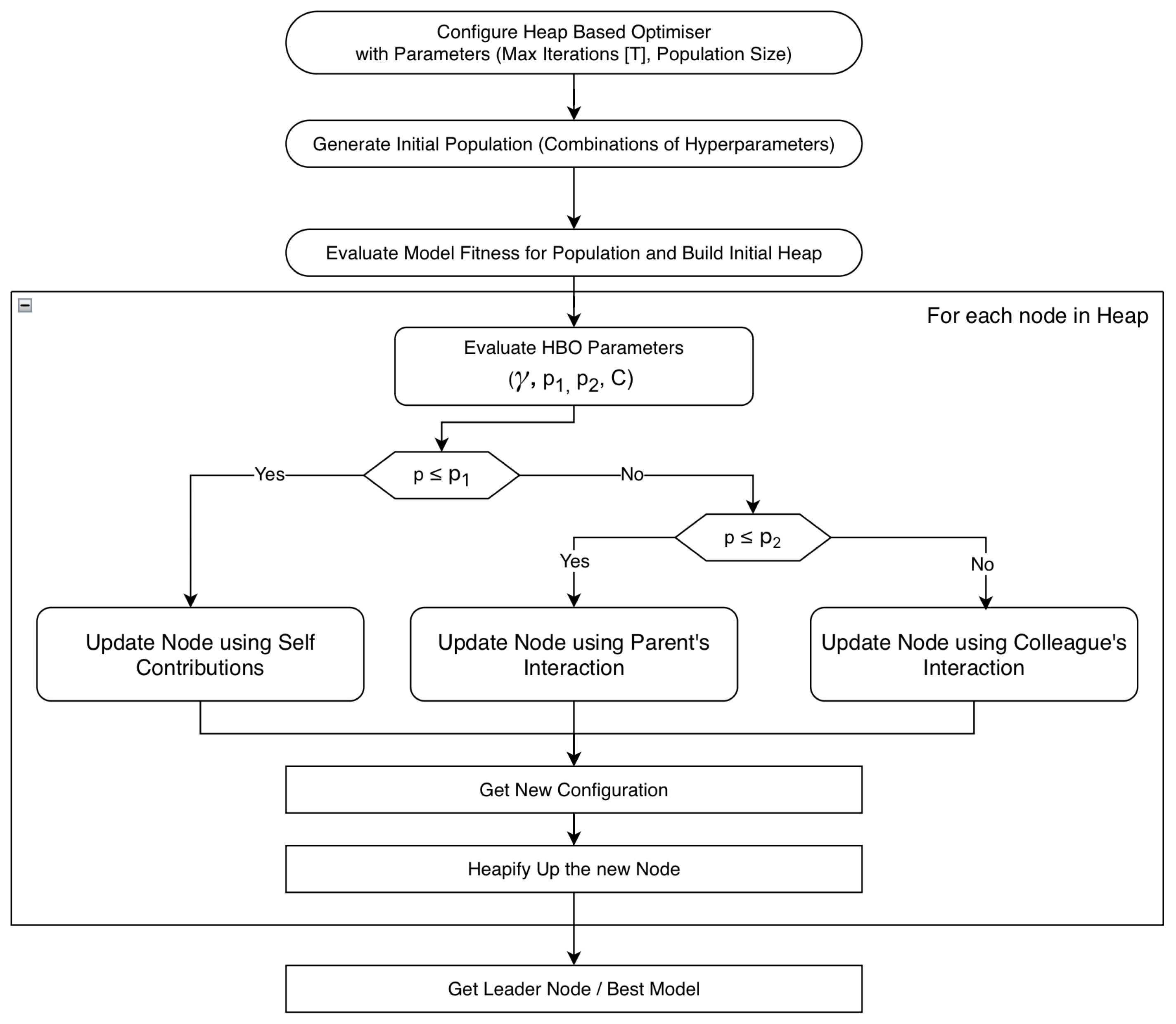
Based on HBO this work proposes HBO-algorithm to tune the hyperparameters of an LSTM network. The algorithm is enumerated below.
1.
Initialise the algorithm with the optimiser parameters like Initial Population Size (Heap Size) and Maximum Iterations (T).
2.
Random-generate the initial population and build the heap structure of Configuration Vectors (Section 2.3).
3.
Update each component of the configuration vector using HBO’s updation policy. After updating all the components in the configuration vector, a new configuration vector that implies a new possible LSTM network has been obtained.
4.
Heapify-Up [23] the newly obtained configuration vector.
5.
Repeat steps 3–4 until T iterations are done.
After the termination of the algorithm, the apex node of the heap denotes the configuration vector which generates the LSTM network with the highest performance. Zhang and Wen, 2022 [28] explore 3 different node updating policies for HBO which shows the versatility of the algorithm. Figure 3 summarises the algorithm as a flowchart.

2.2.2. Genetic Algorithm Based Optimiser

Based on the GA algorithm explored by Gorgolis et al., 2019, Chung and Shin, 2018, Katoch et al., 2021, Lambora et al., 2019 [17,18,29,30], this work proposes GAO-algorithm for tuning hyperparameters of an LSTM network. The algorithm is enumerated below.
1.
Configure the optimiser with its parameters like the number of generations, population size, mutation chance and random selection chance.
2.
Generate the initial population and evaluate the fitness of each of the configuration vectors in the population.
3.
Breed children from two randomly selected parents and either evolve or mutate them to obtain new configuration vectors based on GA parameters Mutation Chance and Random Select Chance. The parents are selected using a uniform random distribution.
4.
Add the children obtained to the population and sort the population based on fitness.
5.
Repeat steps 3–4 until the required number of generations is reached.
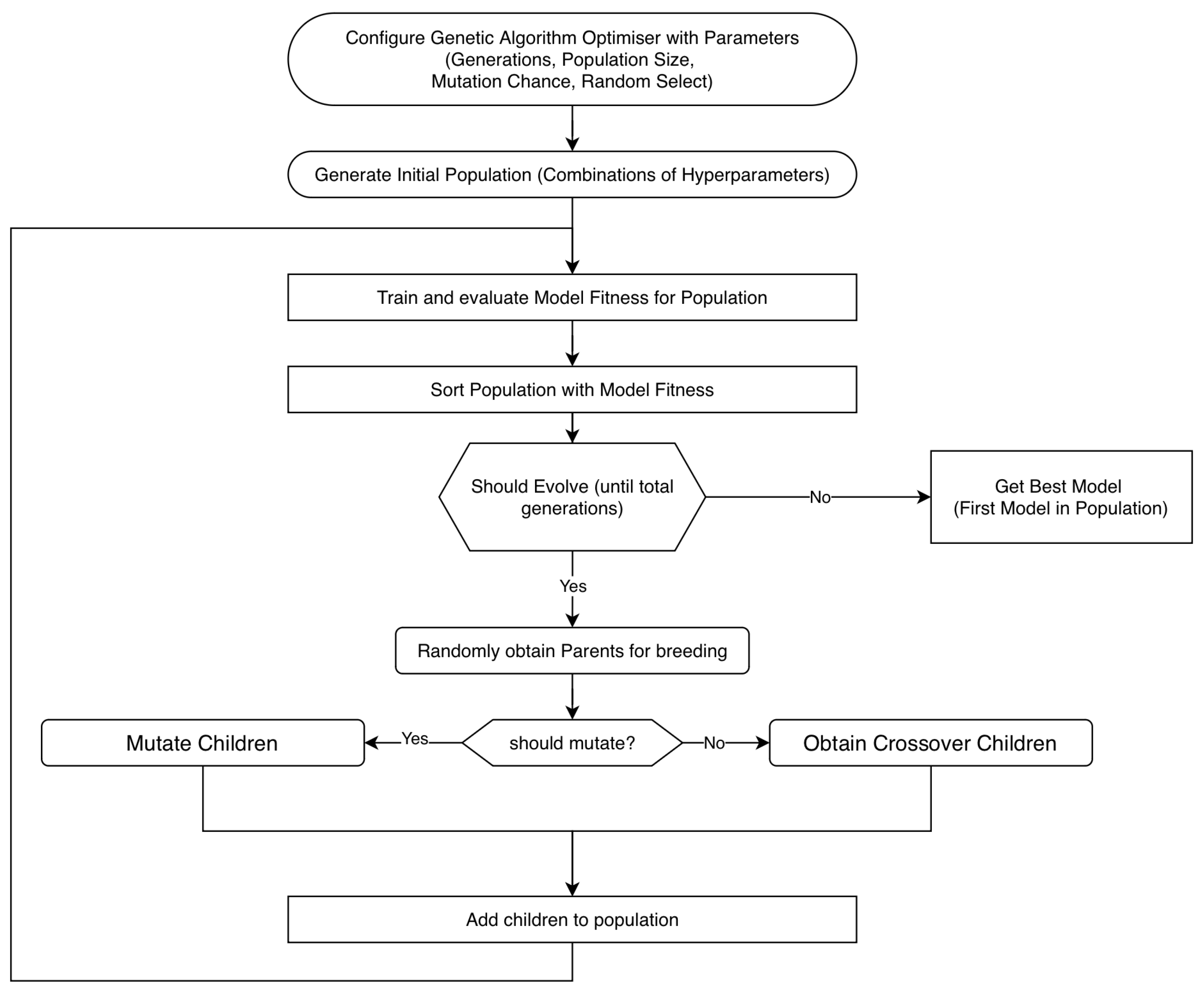
After the termination of the algorithm, the first element in the population denotes the configuration vector which generates the LSTM network with the highest performance. Figure 4 summarises the algorithm in a flowchart.

2.3. Hyperparameter Configuration Space Setup

The hyperparameter configuration space is an n-dimensional functional space which contains the set of all possible combinations of the hyperparameters for the given network. A configuration vector is a vector in the hyperparameter configuration space which represents a unique set of hyperparameters of an LSTM network. The hyperparameter configuration space can become very extensive and may cause the system to become resource intensive. Hence we defined the configuration space for the data used as follows,
Config Vector = B a t c h S i z e s 12 , 24 , 36 , 48 , 108 , 120 L a y e r A c t i v a t i o n relu , elu , tan h , sigmoid M o d e l O p t i m i z e r rmsprop , adam , sgd , adagrad , adadelta , adamax , nadam N o . L S T M L a y e r s 2 , 4 , 6 , 8 , 10 , 12 , 14 , 16 , 18 , 20 N o . L S T M C e l l s 3 , 6 , 12 , 18 , 24 , 36
The total number of possible configuration vectors in the above configuration space is,
Total Configuration Vectors = 6 × 4 × 7 × 10 × 6 = 10,080.
Hence, over 10,000 different LSTM networks can be generated from this configuration space. Training all of these networks would be time-consuming and inefficient, thus, it requires HBO-algorithm and GAO-algorithm to find the optimal configuration vector.

2.4. LSTM Network Properties

After processing the data (Section 2.1.1, Section 2.1.2 and Section 2.1.3) and designing the algorithms for tuning the hyperparameters (Section 2.2.1 and Section 2.2.2), the next step was the LSTM Network’s properties. This is divided as follows:

2.4.1. Network Generation

LSTM Network is generated from a configuration vector by using the hyperparameters represented by the vector. Each component of the configuration vector represents a parameter required to construct and train the LSTM network.

2.4.2. Network Performance Parameters

Network performance parameters are the measures used to analyse and compare the LSTM networks. The following parameters were used in the system:
  • Mean Squared Error (MSE)
    M S E = 1 N i = 1 N ( f i f i ^ ) 2
  • Root Mean Squared Error (RMSE)
    R M S E = 1 N i = 1 N ( f i f i ^ ) 2
  • Mean Squared Logarithmic Error (MSLE)
    M S L E = 1 N i = 0 N ( l o g ( f i + 1 ) l o g ( f i ^ + 1 ) ) 2
  • Coefficient of Determination ( R 2 Score)
    R 2 S c o r e = 1 i = 1 N | f i f i ^ | i = 1 N | f i f m e a n |
  • Model Fitness
    Model Fitness is a custom metric designed to give a balanced R 2 Score in the range of [−100, 100]. Model Fitness was used as the objective/fitness function in both HBO-algorithm and GAO-algorithm for updating the population. Model Fitness is calculated as,
    Model Fitness = R 2 S c o r e × 100 , R 2 Score 0 R 2 S c o r e , 100 R 2 Score < 0 R 2 S c o r e mod 100 , R 2 Score < 100
  • Iteration Fitness
    The Hyperparameter Tuning algorithms (Section 2.2.1 and Section 2.2.2) carry out their operations in multiple steps which are repeated a certain number of times. Each such cycle is known as Iteration. Hence, Iteration Fitness is defined as the average Model Fitness of the entire population for any particular iteration. This metric helps to understand the performance of the algorithm in improving the Model Fitness of the population collectively.
    Iteration Fitness = i Model Fitness i n ( population )
    where Model Fitnessi refers to the fitness of the ith configuration vector in the population and n (population) is the total number of elements in the population.
In Equations (3)–(6) f i represents the forecast obtained from the model and f i ^ refers to the actual solar irradiance value. N refers to the total length of the forecast made.

2.4.3. Optimised LSTM Network Training Setup

The entire data set consisted of 414 columns of time series data with an interval of 5 min between each record. The dataset was divided into a 75–25% (3:1) training-to-testing split ratio. Finally, Python (and its libraries) was used to process the input data, split the data into HF and LF components, design and develop the hyperparameter tuning algorithms and define the hyperparameter configuration space. Python-Keras was used to generate, train and test the LSTM networks. Once the LSTM Network properties have been defined, the next step was to set up the training process using the hyperparameter tuning algorithms designed in Section 2.2.1 and Section 2.2.2. Before starting with the training of the network the optimiser must be configured with its parameters to aid it in finding the optimal hyperparameters. The first block of the flowcharts in Figure 3 and Figure 4 represents this step. No network is trained explicitly by the system to reduce the time required to search the optimal hyperparameters. After randomly generating the initial population (Step 2 in algorithms in Section 2.2.1 and Section 2.2.2), the networks are trained only when the algorithm requires the Model Fitness of the network to evaluate its position and viability in the population. This helps in avoiding unnecessary training of multiple networks while tuning the hyperparameters of the network, which saves time and resources.

3. Results and Discussions

After processing the data (Section 2.1), designing optimisers (Section 2.2), setting up hyperparameter configuration space (Section 2.3), setting the LSTM Network Properties and the optimised training process for the LSTM networks (Section 2.4), the next step was evaluation and analysis of the entire process and its outcome. This section is divided into the following sub-sections:

3.1. Comparison of Frequencies for Data Decomposition

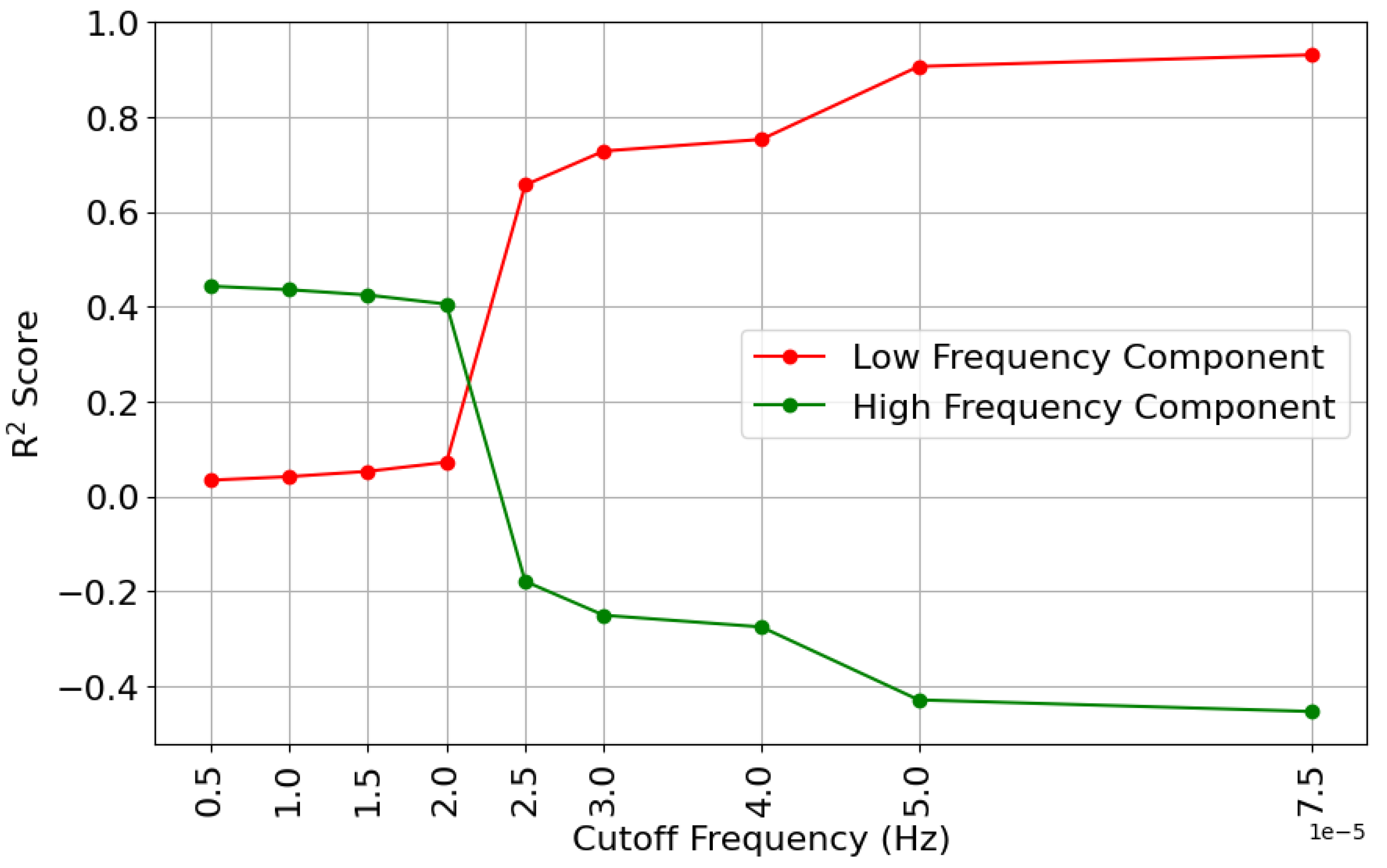
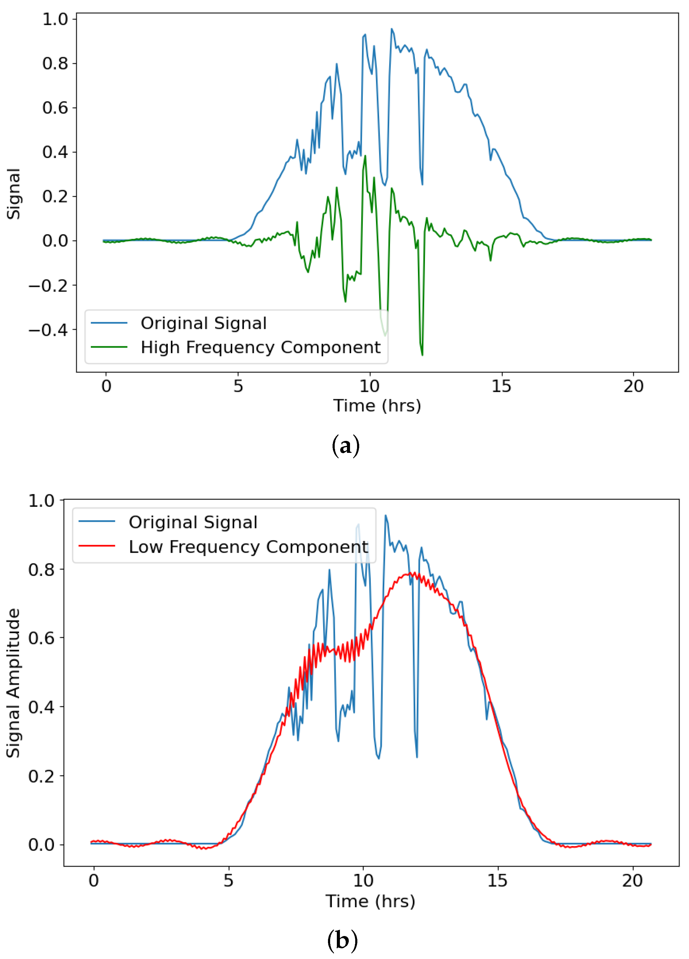
In Section 2.1.3, the procedure for analysing the data using FFT and splitting the data into HF and LF components is defined. Figure 2 shows the FFT plot for the raw data. The frequencies are very low in value because the digital signal is sampled every 5 min or 300 s. Hence the sampling frequency is 1 / 300 samples/second. To identify the frequency which would best split the data into two unique components R 2 Score between the original signal and HF and LF signals for different frequencies was plotted. Figure 5 shows the plot of R 2 Score versus different frequencies for HF and LF components. Table 1 enumerates the same for a wider range of frequencies. After a detailed analysis of the results obtained, it was found that 0.000225 Hz was the best frequency to split the data. The HF and LF components post data decomposition using FFT with a frequency of 0.000225 Hz are shown in Figure 6. These HF and LF components correspond to two different aspects of the input signal. The LF component can be perceived as the daily trend (daily swing) in solar irradiance. Thus, it helps in understanding the approximate change in irradiance as the day progresses. The HF component can be perceived as random changes in solar parameters (like illumination, cloud cover, attenuation et cetera.) which affect the irradiance constantly. However, no relevant works were found to support these arguments.

3.2. Comparison of Optimisers

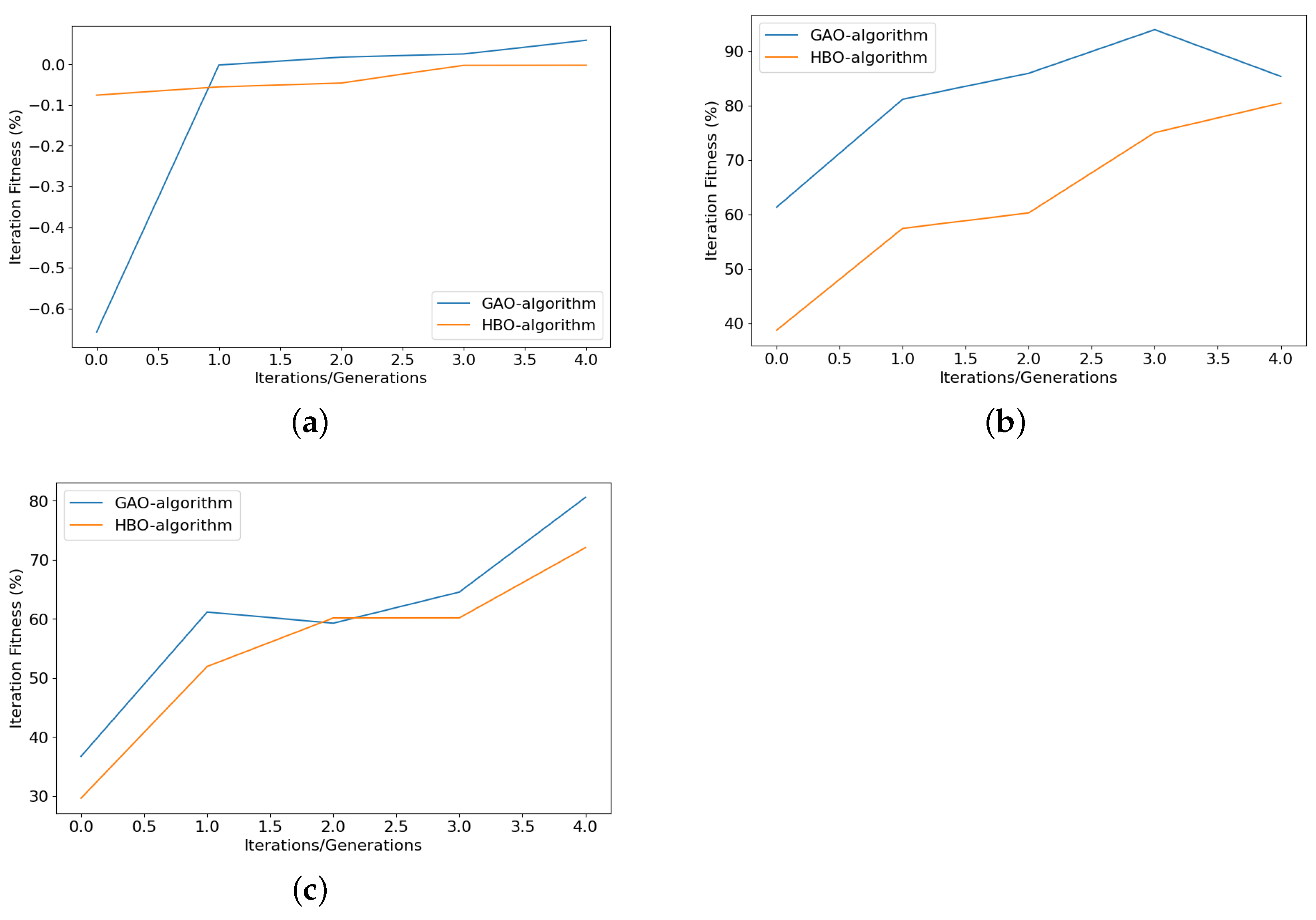
The LSTM Networks were trained using the algorithms designed in Section 2.2.1 and Section 2.2.2. The performance of the algorithms over each iteration was compared using the Iteration Fitness metric defined in Section 2.4.2. Iteration Fitness for each iteration was obtained from both algorithms and compared to observe the improvement in the fitness of the entire population as the algorithm processed it in successions. Figure 7 shows the Iteration Fitness plot for HF, LF and Original data sets.
From Figure 7 it can be observed that the algorithms improve the average efficiency of the population of models present significantly. HBO-algorithm uses a carefully designed parameter C which is calculated as C = T / 25 [23]. Hence it assumes that the Total Number of Iterations is well over 25. Hence HBO’s performance may be undermined due to the limited number of iterations (5 iterations). But this must be limited on the upper end as well. Similar to Bischl et al., 2021 [14], it was observed that long hyperparameter tuning algorithm runs may lead to biased performance estimators and choosing an incorrect set of hyperparameters. Longer runs also implies that a higher amount of resources must be allocated. Hence, the number of iterations must be chosen carefully to avoid either of the above-mentioned conditions.
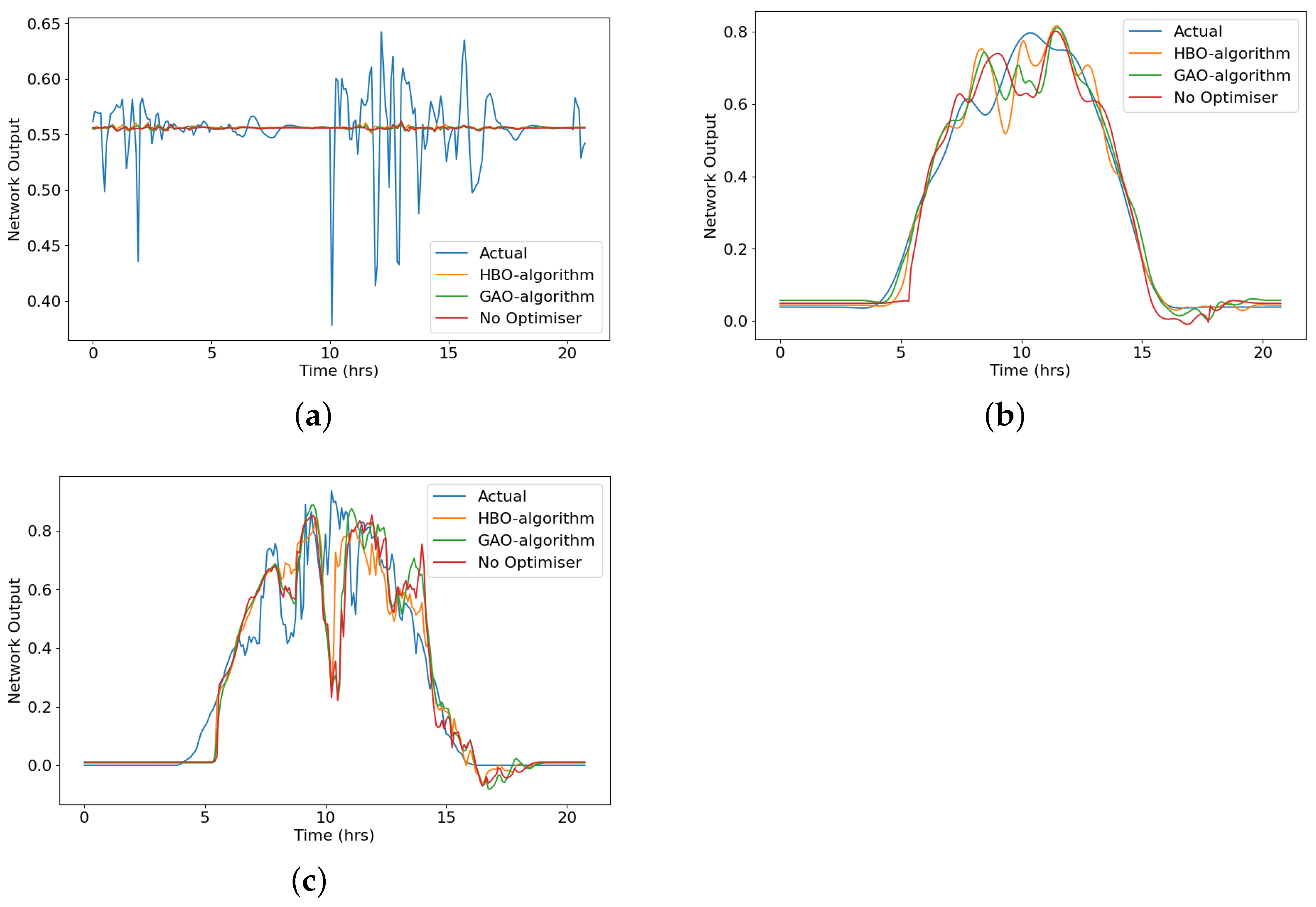
The performance of these optimisers is also compared by using networks trained with 3 different input time series data: High Frequency Data, Low Frequency Data and Original Data. These time series data were obtained from the procedures in Section 2.1.3 and Section 3.1. Table 2 shows the error comparisons between the optimisers in detail. The HF data, decomposed from the Original data, gave similar results in all three cases presented in Table 2. This phenomenon can be attributed to the highly varying nature of the data (shown in Figure 6a. Each of the models used in the study, forecasted HF data close towards the mean value as shown in Figure 8a.

3.3. Effect of Data Decomposition versus Tuning Algorithms

It was also important to understand the effect of data decomposition along with the effect of different tuning algorithms. Furthermore, it is crucial to compare these effects against each other to ensure that the best possible effect on the network is obtained and hence the best possible performance from the network is achieved. This section details the effect of data decomposition against the effect of tuning algorithms using the fitness function defined in Section 2.4.2, Model Fitness. Table 3 shows the Model Fitness based comparison. It was observed that the model fitness for High-Frequency Data is much lower than what was obtained for Low Frequency and Original data sets, similar to the results obtained in Section 3.2.
The results obtained in Table 3 have been analysed using previous works done for short-term and long-term solar energy forecasting. In Fentis et al., 2017 [31], Feed Forward Neural Networks trained with Levenberg-Marquardt algorithm for 15 min ahead short-term forecasts achieving a best R 2 Score of 0.96 (eq. 96% Model Fitness). In Elsaraiti and Merabet, 2022 [32], LSTMs have been employed to obtain 30 min ahead forecast with R 2 Score of 0.745 (eq. 74.5% Model Fitness). Serttas et al., 2018 [33] proposed and implemented the Mycielski-Markov model achieving a R 2 Score of 0.8749 (eq. 87.49% Model Fitness). In Haider et al., 2022 [34], Artificial Neural Networks (ANN), Convolutional Neural Networks (CNN) and LSTM have been used to forecast 1 h, 3 h, 6 h and 12 h ahead. Haider et al., 2022 [34] achieved the highest values of R 2 Scores of 0.984 (98.4%) and 0.913 (91.3%) for 1 h and 3 h ahead forecasts using LSTM. LSTM struggled to perform adequately for forecast horizons of 6 and 12 h ahead obtaining low R 2 Scores less than 0.5 (50%). ANN and CNN performed similarly to LSTM for 1 h and 3 h ahead forecasts but performed significantly better for 6 h and 12 h ahead forecast horizons achieving consistent R 2 Scores above 0.8 (80%). According to the survey conducted by Lai et al., 2020 [35], the average R 2 Score obtained in the solar energy forecasting literature was 0.9240 (92.4%). Liu et al., 2022 [36] used LSTMfusion model for Leaf-Area Index (LAI) and obtained the highest R 2 score of 0.73 (73.0%) between retrieved and aggregated reference LAI on multiple ground-measured dates in 2016. Along similar lines, the HBO-algorithm LSTM Network trained with decomposed data in our work achieved the best Model Fitness of 95.278% for 90 min-ahead forecasts. However, the Model Fitness (and hence R 2 Scores) was found to vary with the nature of data input to the system and hence is data-dependent, similar to the conclusions drawn in [32,33,34,35].
To study these effects even further, Figure 8 shows the forecasted values by the networks generated against the actual values.
From Table 2 and Table 3, it can be observed that High Frequency Data proved to be difficult to forecast. It can be seen that HBO-algorithm gave a better network for more data inputs. The following observations were made from the experiments carried out:
1.
High-Frequency Data produces the lowest amount of errors (from Table 2) but this can be misleading. After checking the Model Forecast Plot in Figure 8 and Model Fitness from Table 3 it was verified that the High-Frequency Data causes the system to forecast the mean value of data and hence the low error but a flat line forecast and very low model fitness.
2.
Low-Frequency Data produces the best Model Fitness (from Table 3). This can be verified using Figure 8.
3.
Original Data produces the highest error (amongst the 3 data sets). This is explained by the fact that original data contains characteristics from both high-frequency and low-frequency data. The Model Fitness is also a little lower than Low Frequency but much higher than High-Frequency Data.

3.4. Further Discussions

The analysed and assessed workings and results indicate that the optimised training process based on Tuning Algorithms/Optimisers presented in this paper along with Data Decomposition improves the LSTM network’s performance significantly. In comparison to the references and previously done works, HBO-algorithm optimised LSTM Network with decomposed data offered reductions in RMSE by 53.42%, 78.30% in MSE and 79.07% in MSLE as compared to the default LSTM network (without data decomposition and no optimiser applied to it). It achieved the highest fitness of 95.278% for 90 min ahead forecast. GAO-algorithm LSTM Network with data decomposition also gave promising results slightly behind HBO with 94.38% fitness. Furthermore, the tuning algorithms may be combined and used in parallel to allow the system to train the Network which captures a wider variety of trends and characteristics as both the optimisers are sensitive to data differently (Figure 8). Zou and Yang, 2004 [3] and Wang et al., 2022 [37] also share similar insights on combining different models in order to capture more information from the available data.

4. Conclusions

The majority of the works conducted in this domain previously have concluded that the performance can be improved by tuning the hyperparameters of their models. However, Hyperparameter Tuning faces several problems due to the absence of a proper system which can tune the hyperparameters efficiently and hassle-free. For the first time, this paper introduced two different algorithms, based on proven optimisation algorithms, to efficiently find the optimal set of hyperparameters for an LSTM Network and the Data Decomposition technique using FFT to improve the performance of the network. Similar to results obtained in Shahid et al., 2021 [38] this work also concluded that adding optimising algorithms positively and significantly impacts the network’s performance provided the optimal number of iterations and optimiser parameters are used.
Thus, Hyperparameter Tuning (along with data decomposition) becomes a crucial technique in addition to other state-of-the-art techniques to improve the training efficiency and performance of the models. The assessments and analysis of these algorithms can be further improved by studying and applying them to a wider variety of data and adapting them to different types of models which require hyperparameter tuning.

Author Contributions

Conceptualization, H.D.; Methodology, H.D.; Software, H.D.; Validation, Y.K. and P.K.; formal analysis, H.D.; investigation, H.D.; resources, Y.K.; data curation, Y.K.; writing—original draft preparation, H.D.; writing—review and editing, Y.K. and P.K.; visualization, H.D.; supervision, Y.K. and P.K. All authors have read and agreed to the published version of the manuscript.

Funding

This research received no external funding.

Data Availability Statement

All data sets used and produced for the purposes of this study can be requested from the corresponding authors.

Acknowledgments

P.K. acknowledges the EU-funded CiROCCO project under Grant Agreement No 101086497. The authors would like to thank National Institute of Technology Karnataka for providing the facilities to conduct this research work.

Conflicts of Interest

The authors declare no conflict of interest.

Abbreviations

The following abbreviations are used in this manuscript:
LSTMLong Short Term Memory
HBOHeap Based Optimiser
GAOGenetic Algorithm Optimiser
MLMachine Learning
NNsNeural Networks
AIArtificial Intelligence
ARIMAAuto Regression Integrated Moving Average
RNNsRecurrent Neural Networks
GAGenetic Algorithm
CRHCorporate Ranking Hierarchy
HFHigh Frequency
LFLow Frequency
FFTFast Fourier Transform
MSEMean Squared Error
RMSERoot Mean Squared Error
MSLEMean Squared Logarithmic Error

References

  1. Sharma, V.; Yang, D.; Walsh, W.; Reindl, T. Short term solar irradiance forecasting using a mixed wavelet neural network. Renew. Energy 2016, 90, 481–492. [Google Scholar] [CrossRef]
  2. Wang, Q.; Li, S.; Li, R. Forecasting energy demand in China and India: Using single-linear, hybrid-linear, and non-linear time series forecast techniques. Energy 2018, 161, 821–831. [Google Scholar] [CrossRef]
  3. Zou, H.; Yang, Y. Combining time series models for forecasting. Int. J. Forecast. 2004, 20, 69–84. [Google Scholar] [CrossRef]
  4. Clements, M.P.; Franses, P.H.; Swanson, N.R. Forecasting economic and financial time-series with non-linear models. Int. J. Forecast. 2004, 20, 169–183. [Google Scholar] [CrossRef]
  5. Koudouris, G.; Dimitriadis, P.; Iliopoulou, T.; Mamassis, N.; Koutsoyiannis, D. A stochastic model for the hourly solar radiation process for application in renewable resources management. Adv. Geosci. 2018, 45, 139–145. [Google Scholar] [CrossRef]
  6. Colak, I.; Yesilbudak, M.; Genc, N.; Bayindir, R. Multi-period prediction of solar radiation using ARMA and ARIMA models. In Proceedings of the 2015 IEEE 14th International Conference on Machine Learning and Applications (ICMLA), Miami, FL, USA, 9–11 December 2015; IEEE: Piscataway, NJ, USA, 2015; pp. 1045–1049. [Google Scholar]
  7. Shadab, A.; Ahmad, S.; Said, S. Spatial forecasting of solar radiation using ARIMA model. Remote Sens. Appl. Soc. Environ. 2020, 20, 100427. [Google Scholar] [CrossRef]
  8. Meenal, R.; Binu, D.; Ramya, K.; Michael, P.A.; Vinoth Kumar, K.; Rajasekaran, E.; Sangeetha, B. Weather forecasting for renewable energy system: A review. Arch. Comput. Methods Eng. 2022, 29, 2875–2891. [Google Scholar] [CrossRef]
  9. Siami-Namini, S.; Tavakoli, N.; Siami Namin, A. A Comparison of ARIMA and LSTM in Forecasting Time Series. In Proceedings of the 2018 17th IEEE International Conference on Machine Learning and Applications (ICMLA), Orlando, FL, USA, 17–20 December 2018; pp. 1394–1401. [Google Scholar] [CrossRef]
  10. Rahimzad, M.; Moghaddam Nia, A.; Zolfonoon, H.; Soltani, J.; Danandeh Mehr, A.; Kwon, H.H. Performance comparison of an LSTM-based deep learning model versus conventional machine learning algorithms for streamflow forecasting. Water Resour. Manag. 2021, 35, 4167–4187. [Google Scholar] [CrossRef]
  11. Yu, Y.; Si, X.; Hu, C.; Zhang, J. A Review of Recurrent Neural Networks: LSTM Cells and Network Architectures. Neural Comput. 2019, 31, 1235–1270. [Google Scholar] [CrossRef]
  12. De, V.; Teo, T.T.; Woo, W.L.; Logenthiran, T. Photovoltaic power forecasting using LSTM on limited dataset. In Proceedings of the 2018 IEEE Innovative Smart Grid Technologies-Asia (ISGT Asia), Singapore, 22–25 May 2018; IEEE: Piscataway, NJ, USA, 2018; pp. 710–715. [Google Scholar]
  13. Ewees, A.A.; Al-qaness, M.A.; Abualigah, L.; Abd Elaziz, M. HBO-LSTM: Optimized long short term memory with heap-based optimizer for wind power forecasting. Energy Convers. Manag. 2022, 268, 116022. [Google Scholar] [CrossRef]
  14. Bischl, B.; Binder, M.; Lang, M.; Pielok, T.; Richter, J.; Coors, S.; Thomas, J.; Ullmann, T.; Becker, M.; Boulesteix, A.L.; et al. Hyperparameter optimization: Foundations, algorithms, best practices, and open challenges. Wiley Interdiscip. Rev. Data Min. Knowl. Discov. 2021, 13, e1484. [Google Scholar] [CrossRef]
  15. Falkner, S.; Klein, A.; Hutter, F. BOHB: Robust and efficient hyperparameter optimization at scale. In Proceedings of the International Conference on Machine Learning, PMLR, Stockholm, Sweden, 10–15 July 2018; pp. 1437–1446. [Google Scholar]
  16. Bergstra, J.; Bardenet, R.; Bengio, Y.; Kégl, B. Algorithms for hyper-parameter optimization. In Advances in Neural Information Processing Systems; Curran Associates Inc.: Sydney, NSW, Australia, 2011; Volume 24. [Google Scholar]
  17. Gorgolis, N.; Hatzilygeroudis, I.; Istenes, Z.; Gyenne, L.G. Hyperparameter optimization of LSTM network models through genetic algorithm. In Proceedings of the 2019 10th International Conference on Information, Intelligence, Systems and Applications (IISA), Patras, Greece, 15–17 July 2019; IEEE: Piscataway, NJ, USA, 2019; pp. 1–4. [Google Scholar]
  18. Chung, H.; Shin, K.S. Genetic algorithm-optimized long short-term memory network for stock market prediction. Sustainability 2018, 10, 3765. [Google Scholar] [CrossRef]
  19. Ali, M.A.; P.P., F.R.; Abd Elminaam, D.S. An Efficient Heap Based Optimizer Algorithm for Feature Selection. Mathematics 2022, 10, 2396. [Google Scholar] [CrossRef]
  20. AbdElminaam, D.S.; Houssein, E.H.; Said, M.; Oliva, D.; Nabil, A. An efficient heap-based optimizer for parameters identification of modified photovoltaic models. Ain Shams Eng. J. 2022, 13, 101728. [Google Scholar] [CrossRef]
  21. Abdel-Basset, M.; Mohamed, R.; Elhoseny, M.; Chakrabortty, R.K.; Ryan, M.J. An efficient heap-based optimization algorithm for parameters identification of proton exchange membrane fuel cells model: Analysis and case studies. Int. J. Hydrogen Energy 2021, 46, 11908–11925. [Google Scholar] [CrossRef]
  22. Ginidi, A.R.; Elsayed, A.M.; Shaheen, A.M.; Elattar, E.E.; El-Sehiemy, R.A. A novel heap-based optimizer for scheduling of large-scale combined heat and power economic dispatch. IEEE Access 2021, 9, 83695–83708. [Google Scholar] [CrossRef]
  23. Askari, Q.; Saeed, M.; Younas, I. Heap-based optimizer inspired by corporate rank hierarchy for global optimization. Expert Syst. Appl. 2020, 161, 113702. [Google Scholar] [CrossRef]
  24. Kumar, A.; Kashyap, Y.; Kosmopoulos, P. Enhancing Solar Energy Forecast Using Multi-Column Convolutional Neural Network and Multipoint Time Series Approach. Remote Sens. 2022, 15, 107. [Google Scholar] [CrossRef]
  25. Jursa, R.; Rohrig, K. Short-term wind power forecasting using evolutionary algorithms for the automated specification of artificial intelligence models. Int. J. Forecast. 2008, 24, 694–709. [Google Scholar] [CrossRef]
  26. Heckbert, P. Fourier transforms and the fast Fourier transform (FFT) algorithm. Comput. Graph. 1995, 2, 15–463. [Google Scholar]
  27. Sevgi, L. Numerical Fourier transforms: DFT and FFT. IEEE Antennas Propag. Mag. 2007, 49, 238–243. [Google Scholar] [CrossRef]
  28. Zhang, X.; Wen, S. Heap-based optimizer based on three new updating strategies. Expert Syst. Appl. 2022, 209, 118222. [Google Scholar] [CrossRef]
  29. Katoch, S.; Chauhan, S.S.; Kumar, V. A review on genetic algorithm: Past, present, and future. Multimed. Tools Appl. 2021, 80, 8091–8126. [Google Scholar] [CrossRef] [PubMed]
  30. Lambora, A.; Gupta, K.; Chopra, K. Genetic algorithm-A literature review. In Proceedings of the 2019 International Conference on Machine Learning, Big Data, Cloud and Parallel Computing (COMITCon), Faridabad, India, 14–16 February 2019; IEEE: Piscataway, NJ, USA, 2019; pp. 380–384. [Google Scholar]
  31. Fentis, A.; Bahatti, L.; Mestari, M.; Chouri, B. Short-term solar power forecasting using Support Vector Regression and feed-forward NN. In Proceedings of the 2017 15th IEEE International New Circuits and Systems Conference (NEWCAS), Strasbourg, France, 25–28 June 2017; IEEE: Piscataway, NJ, USA, 2017; pp. 405–408. [Google Scholar]
  32. Elsaraiti, M.; Merabet, A. Solar power forecasting using deep learning techniques. IEEE Access 2022, 10, 31692–31698. [Google Scholar] [CrossRef]
  33. Serttas, F.; Hocaoglu, F.O.; Akarslan, E. Short term solar power generation forecasting: A novel approach. In Proceedings of the 2018 International Conference on Photovoltaic Science and Technologies (PVCon), Ankara, Turkey, 4–6 July 2018; IEEE: Piscataway, NJ, USA, 2018; pp. 1–4. [Google Scholar]
  34. Haider, S.A.; Sajid, M.; Sajid, H.; Uddin, E.; Ayaz, Y. Deep learning and statistical methods for short-and long-term solar irradiance forecasting for Islamabad. Renew. Energy 2022, 198, 51–60. [Google Scholar] [CrossRef]
  35. Lai, J.P.; Chang, Y.M.; Chen, C.H.; Pai, P.F. A survey of machine learning models in renewable energy predictions. Appl. Sci. 2020, 10, 5975. [Google Scholar] [CrossRef]
  36. Liu, T.; Jin, H.; Li, A.; Fang, H.; Wei, D.; Xie, X.; Nan, X. Estimation of Vegetation Leaf-Area-Index Dynamics from Multiple Satellite Products through Deep-Learning Method. Remote Sens. 2022, 14, 4733. [Google Scholar] [CrossRef]
  37. Wang, J.; Wang, Z.; Li, X.; Zhou, H. Artificial bee colony-based combination approach to forecasting agricultural commodity prices. Int. J. Forecast. 2022, 38, 21–34. [Google Scholar] [CrossRef]
  38. Shahid, F.; Zameer, A.; Muneeb, M. A novel genetic LSTM model for wind power forecast. Energy 2021, 223, 120069. [Google Scholar] [CrossRef]
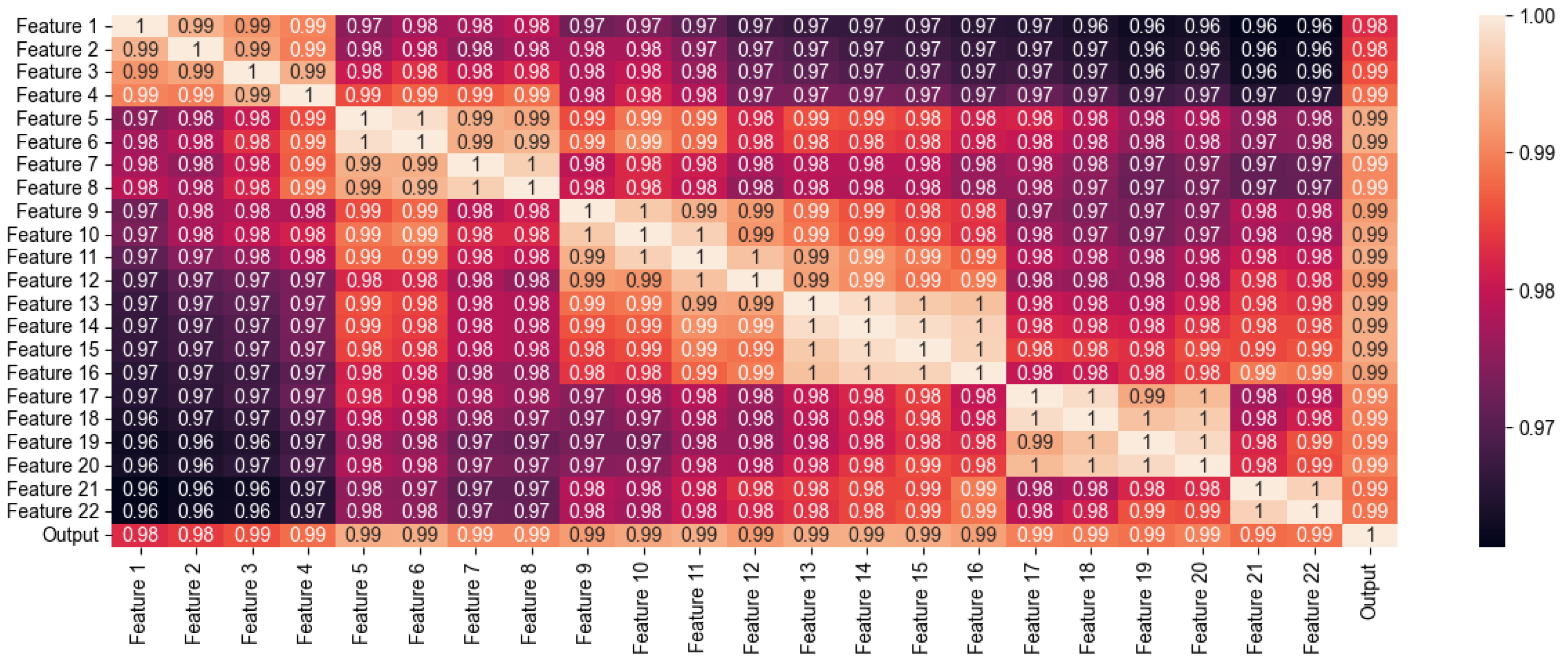
Figure 1. Heat Map of Correlation Matrix between each of the input features and the output variable.
Remotesensing 15 02076 g001
Figure 2. Fourier Transform plot of an input feature, denoting the frequency distribution present in the input signal. The plot is obtained by using Fast Fourier Transform technique.
Remotesensing 15 02076 g002
Figure 3. Flowchart of HBO-algorithm for tuning hyperparameters of LSTM Networks.
Remotesensing 15 02076 g003
Figure 4. Flowchart of GAO-algorithm for tuning hyperparameters of LSTM Networks.
Remotesensing 15 02076 g004
Figure 5. R 2 Score versus Cutoff Frequency used for decomposing the data signal.
Remotesensing 15 02076 g005
Figure 6. Comparison between the original signal and the signals obtained after data decomposition using FFT filtering: (a) High Frequency Component of the original data (b) Low Frequency Component of the original data.
Remotesensing 15 02076 g006
Figure 7. Comparison between HBO-algorithm and GAO-algorithm using Iteration Fitness Performance parameter for 5 iterations (5 generations for GAO-algorithm): (a) Iteration Fitness for High Frequency Component of the original data (b) Iteration Fitness for Low Frequency Component of the original data (c) Iteration Fitness for the original data.
Remotesensing 15 02076 g007
Figure 8. Comparison of HBO-algorithm, GAO-algorithm, No Optimiser LSTM Networks 90 min ahead Forecasts with actual output values: (a) Forecast of High Frequency Component of original data (b) Forecast of Low Frequency Component of original data (c) Forecast of original data.
Remotesensing 15 02076 g008
Table 1. R 2 Score versus Cutoff Frequencies.
Cutoff FrequencyLow Frequency Signal (%)High Frequency Signal (%)
0.5 × 10 5 Hz3.4044.32
1 × 10 5 Hz4.1543.57
1.5 × 10 5 Hz5.2742.45
2 × 10 5 Hz7.1940.53
2.5 × 10 5 Hz65.64−17.92
3 × 10 5 Hz72.80−25.08
4 × 10 5 Hz75.25−27.54
5 × 10 5 Hz90.64−42.92
7.5 × 10 5 Hz93.09−45.37
1 × 10 4 Hz94.19−46.48
2 × 10 4 Hz95.73−48.02
2.25 × 10 4 Hz95.94−48.22
Table 2. Comparison of Optimisers using Error Parameters for different data inputs.
OptimiserMSERMSEMSLEData Set
Normalised Solar Irradiance × 10 3
HBO-algorithm2.131246.16300.9030High Frequency
3.741161.16021.7730Low Frequency
14.3627119.84357.2800Original
GAO-algorithm2.130946.15390.9021High Frequency
4.453266.73102.1203Low Frequency
17.0361130.52218.3667Original
No Optimiser *2.131946.16170.9034High Frequency
6.829082.63883.3598Low Frequency
17.2401131.30368.4711Original
* No Optimiser based LSTM Network implies the default network generated by Python-Keras.
Table 3. Comparison between Effect of Data Decomposition and Effect of Tuning Algorithms using Model Fitness.
Data SetHBO-AlgorithmGAO-AlgorithmNo Optimiser *
High Frequency0.0888%0.09468%−0.00329%
Low Frequency95.278%94.38%91.38%
Original84.336%81.42%81.20%
* No Optimiser based LSTM Network implies the default network generated by Python-Keras.
Disclaimer/Publisher’s Note: The statements, opinions and data contained in all publications are solely those of the individual author(s) and contributor(s) and not of MDPI and/or the editor(s). MDPI and/or the editor(s) disclaim responsibility for any injury to people or property resulting from any ideas, methods, instructions or products referred to in the content.