Abstract
In this study, a new technique is proposed to retrieve temperature and relative humidity profiles under clear sky conditions in the Arctic region based on the artificial neural network (ANN) algorithm using Fengyun-3D (FY-3D) vertical atmospheric sounder suit (VASS: HIRAS, MWTS-II, and MWHS-II) observations. This technology combines infrared (IR) and microwave (MW) observations to improve retrieval accuracy in the middle and low troposphere by reducing the sensitivity of the neural networks (NNs) to cloud coverage. The approach was compared against other methods available in the literature on retrieving profiles only from FY-3D/HIRAS data. Furthermore, its retrieval performance was tested by comparing the NNs’ prediction accuracy versus the corresponding FY-3D/VASS and Aqua/AIRS L2 products. The results showed that: (1) NNs retrieval accuracy is higher during the warm season and over the ocean; (2) the retrieval accuracy of NNs has been significantly improved compared with satellite L2 products; (3) referring to radiosonde observations, the retrieval accuracy of NNs below 600 hPa is effectively improved by adding the information of the MW channel, especially on land where cloud clearing is more difficult. The root mean square error (RMSE) of temperature and relative humidity in the cold season were reduced by 0.3 K and 2%, respectively. The advanced NNs proposed herein offer a more stable retrieval performance compared with NNs built only by FY-3D/HIRAS data. The study results indicated the potential value in time and space domain of the NN algorithm in retrieving temperature and relative humidity profiles of the Arctic region from FY-3D/VASS observations under clear-sky conditions. All in all, this work enhances our knowledge towards improving operational use of FY-3D satellite data in the Arctic region.
1. Introduction
Climate change in the Arctic has been the focus of scientific research in recent years [1,2,3,4], but the polar climate in this area of the planet is extremely harsh, with low temperatures and ice for many years [5]. The Arctic region has long winters, extremely low temperatures, strong air–sea exchanges, and high humidity, which is manifested as fog. These climate challenges add additional difficulties to the safety of navigation in the Arctic region [6,7]. Therefore, it is important to obtain timely temperature and relative humidity information for the research of the Arctic climate, Arctic scientific expeditions, and the opening of the Arctic shipping route [8,9,10]. Radiosonde observations (RAOB) allow the obtaining of direct measurements of water vapor; yet, the operational RAOB measurements are only performed twice a day at several hundred fixed stations around the world, which makes their temporal and spatial resolutions have important limitations [11]. Climate change research lacks a set of three-dimensional temperature and relative humidity field data with high spatial and temporal resolution in the Arctic region. Meteorological satellite remote sensing can make up for the shortcomings of conventional observation. Additionally, satellite-borne hyperspectral infrared remote sensing technology is expected to achieve high spatial and temporal resolution and high precision detection of atmospheric temperature and humidity field [12,13,14,15,16,17,18,19].
A previous study by [20] demonstrated that temperature and relative humidity profiles under clear sky conditions in the Arctic region can be retrieved from FY-3D/HIRAS’ 219 channel observations based on artificial neural networks (ANN). Authors showed that a root mean square error (RMSE) of NN retrievals can be reached within 1 K in the middle and upper troposphere. They also underlined that the retrieval performance in the lower troposphere still needs to be improved. Although FY-3D/MERSI-II L2 cloud products [21,22] have been used to eliminate the pixels of HIRAS affected by clouds, due to the accuracy of MERSI-II cloud products, all selected HIRAS’FOVs (fields of view) cannot be completely unaffected by clouds that can weaken the observation ability of the infrared (IR) measurements. Furthermore, cloud clearing problems on land are more difficult than those in the ocean due to the influence of surface emissivity, and the Arctic region has been covered by clouds for a long time [23,24]. Therefore, there is a need to develop approaches that will help us reduce the influence of clouds on HIRAS’FOVs. Spaceborne microwave (MW) and infrared (IR) sounding instruments have enabled significant improvements in weather forecast accuracy. The IR measurements have high spectral resolution but are strongly affected by clouds, while the lower resolution MW measurements have far less sensitivity to clouds [25,26].
In purview of the above, in the present study a new method is proposed to retrieve temperature and relative humidity profiles under a clear sky in the Arctic region. In the method, in addition to FY-3D/HIRAS data, FY-3D/MWTS-II and MWHS-II observations [27,28] are also added into the input layer of NNs to enable NNs to obtain high precision results while reducing the influence of clouds on NNs in retrieving data. The proposed method is able to retrieve atmospheric temperature and relative humidity profile regions based on a NN algorithm from FY-3D/VASS data. The methods’ retrieval performance is compared with that obtained from NNs built only by FY-3D/HIRAS observations to evaluate the improvement of retrieval accuracy by using IR and MW measurements. Furthermore, additional comparisons are performed to assess the accuracy of the NNs’ retrievals against FY-3D/VASS and Aqua/AIRS L2 products with the ERA5 temperature and humidity profiles as the reference standard. The scheme proposed herein for improving the retrieval performance of the middle and low troposphere in the Arctic region is proved to be feasible, and can provide a potential prospect for the application of FY-3D satellite data in a wide range of practical value and research investigations.
2. Data
2.1. Satellite Data
FengYun-3D is a Chinese second-generation sun-synchronous meteorological satellite. Herein, observations from the FY-3D/VASS (HIRAS, MWTS-II, MWHS-II) L1-level brightness temperature (BT) covering the region north of 60°N from May 2019 to April 2020 were used as input data for NN modeling in this study. FY-3D/HIRAS is the first infrared Fourier detection instrument carried on FY-3D [29,30]. The field angle of each probe observation is 1.1°, and the instantaneous field size of the ground at the corresponding sub-point is about 16 km. FY-3D/MWTS-II [28,31,32,33] uses oxygen absorption bands at 50–60 GHZ to detect atmospheric temperature profiles and a total of 13 channels are used for earth exploration. The instantaneous field size of the ground at the corresponding sub-point is about 33 km. The sensitivity of the instrument is 0.3~2.1 K, and the calibration accuracy is 1.5 K. FY-3D/MWHS-II [34,35] uses 15 channels to achieve all-weather observation of the vertical distribution of global atmospheric relative humidity, water vapor, and rainfall, which plays an important role in atmospheric detecting. The instantaneous field size of the ground at the corresponding sub-point is about 25 km for Channel 1–9 and 15 km for 10–15. It uses 89 GHz, 118 GHz, 150 GHz, and 183 GHz frequencies for Earth detection. Window channels at 89 GHz and 150 GHz can be used for precipitation recognition, channels near 118 GHz oxygen absorption line are used for the vertical detection of atmospheric temperature, and channels near the 183 GHz water vapor absorption line are used to obtain more detailed information about the vertical distribution of atmospheric water vapor. All the FY-3D/VASS L1 data used in our study can be obtained for free from the National Satellite Meteorological Center (http://satellite.nsmc.org.cn/PortalSite/Data/Satellite.aspx, accessed on 1 May 2019) after user registration.
2.2. Atmospheric Profile Data
The profile data collected from May 2019 to April 2020 at 00:00, 12:00 UTC in the Arctic are from European Centre for Medium-Range Weather Forecasts (ECMWF) ERA5 [36,37,38] temperature and relative humidity fields, and radiosonde observations (RAOBs) during the same period in the Arctic are from the University of Wyoming. The spatial resolution of the ERA5 is 0.25° × 0.25°. All the data can be obtained at no cost. Although RAOBs are the closest to the real state of the atmosphere at present, the disadvantages, such as lower spatial and temporal resolution, lack of radiosondes over the ocean and so on, make it difficult to achieve enough data in the Arctic under clear sky conditions. Therefore, ERA5 data were used in the NNs training process and the observations from 51 stations on land were used for validation. Prior to modeling, ERA5 profiles in the Arctic region were validated against RAOBs on land based on 7760 matched samples: 2844 samples during the warm season and 4925 samples during the cold season.
Figure 1 illustrates the comparison results between ERA5 profiles and RAOBs during the warm season. The RMSE of temperature is within 1 K at all levels except for the bottom two levels and the maximum is about 1.4 K. With the increase of the height to 400 hPa, RMSE gradually decreases to basically around 0.5 K, and mean bias (ME) is also around 0 K. RMSE increases to 1.2 K around 200 hPa. The difference of relative humidity at this level is also obvious. This pressure level is located at the junction of troposphere and stratosphere in the Arctic region, with strong small scale and complex weather conditions, leading to a large difference between ERA5 and RAOBs. The right column of Figure 1 shows that, compared with ERA5, the relative humidity (RH) of RAOBs is significantly larger in troposphere and smaller in stratosphere. ME varies between 0 and 5%, and RMSE varies between 10 and 15% in the middle and lower troposphere, where most of the water vapor is concentrated.
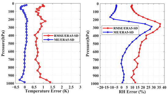
Figure 1.
Deviation of temperature and RH between ERA5 and RAOBs during warm season.
Figure 2 shows the comparison results between ERA5 profiles and RAOBs during the cold season. Compared with the results in the warm season, the deviation in the cold season is larger below 900 hPa. The RMSE of temperatures at 985.88 hPa and 957.44 hPa is also larger than that at other pressure levels, and the maximum is about 2 K. RMSE basically stays within 1 K with the increase in height to 100 hPa. Relative humidity errors with heights between the two kinds of data are basically consistent with those in summer. The trend of RH RMSE and ME with height is consistent with that in the warm season, but the deviation is still larger than that in the warm season.
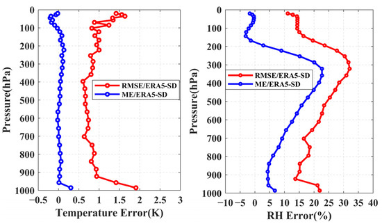
Figure 2.
Deviation of temperature and RH between ERA5 and RAOBs during cold season.
3. Methods
3.1. Data Pre-Processing
FY-3D/VASS L1 data and atmospheric profile data were first pre-processed. HIRAS’ pixels with cloud amounts less than 5% were selected by using FY3D/MERSI-II L2 cloud products [20], which are considered as cloudless, and interpolated MWTS-II and MWHS-II observations to HIRAS clear sky pixels by using the inverse distance weight method [39,40]. The ERA5 data were matched with HIRAS data in time and space, which required that the distance between HIRAS FOVs and ERA5 was less than 0.1°, and the time difference between ERA5 and HIRAS data was less than 1 h. In order to make the training set of different models more representative and reduce the training difficulty of the NNs, brightness temperature and training targets were classified using two variables: season (warm season: May 2019 to October 2019; cold season: November 2019 to April 2020) and surface type (ocean and land).
Based on the above re-processing method, 38,307 and 49,842 clear-sky samples on land and ocean north of 60°N were matched, respectively. Samples were divided according to the climate characteristics of the Arctic region. In total, 20% of the samples were divided for testing NNs and 80% of the samples were divided for training. The samples obtained are shown in Table 1, and the data distribution is shown in Figure 3, which is the map of the Arctic using polar stereographic projections with all matched samples distributed in the north 60°N. The RAOBs were collocated to NNs retrievals within 100 km [30]. As the fact that most radiosondes in the Arctic cannot detect above 50 hPa, the comparisons with RAOBs were only performed between 50 and 1000 hPa (28 layers) to increase the sample number for comparison. Additionally, the number of collocations is summarized in Table 2, and the specific retrieval layers are listed in Table 3.

Table 1.
Data set for neural networks acquired under clear sky conditions in the Arctic.
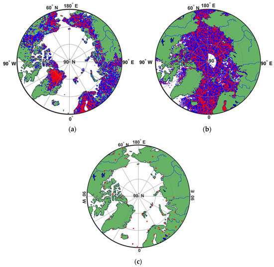
Figure 3.
(a,b) Distribution of samples used to build retrieval models on land and ocean under clear sky, respectively. Blue dots represent training samples; red dots represent validation samples. (c) Distribution of 51 radiosonde stations in the Arctic. The red solid dots represent the radiosonde stations.
Table 2.
Number of collocated RAOB datasets on land. (T represents temperature, RH represents relative humidity).
Table 3.
Specific retrieval pressure layers from 1 to 1000 hPa.
3.2. Construction of BP Neural Network
Back-propagation (BP) neural network [41,42] is a multi-layer feedforward network trained by the error back-propagation algorithm, and is one of the most widely used neural network models at present. BP neural networks are also widely used in meteorological research, and have been successfully used in atmospheric parameter inversion [43,44,45,46]. It is a relatively mature and widely used non-linear inversion algorithm. In a previous study by [20], the method of using 219 channels of HIRAS to obtain the optimal NNs with 220 input neurons (brightness temperature of 219 channels and the sensor zenith angle) was proposed. There are 250 input nodes of the improved NNs adding MW data studied in this work (NNs-250: 219 HIRAS channels, 13 MWTS channels, 15 MWHS channels, and 3 zenith angles). The output layer of the NNs still has 42 nodes, which represent 42 vertical atmospheric layers from 1 to 1000 hPa. To ensure that changes in the accuracy of retrievals are due to the addition of MW data to the maximum extent, the same method of constructing NNs in our previous study [20] was used: selecting the hyperbolic tangent S-type tansig as the transfer function and trainscg as the training algorithm, and the number of hidden layer nodes increased from 300 to 360 using the same method [47].
The statistical metrics used to evaluate the retrieval performance of the NNs-250 included the correlation coefficient (R), the root mean square error (RMSE), and the mean bias (ME) between the retrievals and the true value. Their mathematical expressions are shown below:
where n represents the number of samples, is the inversion profile, and is the true value.
4. Retrieval Performance as Compared with ERA5
4.1. Validation of NNs-250 with ERA5
The temperature retrievals in the statistics came from 42 pressure levels (1–1000 hPa), and the results are shown in Figure 4. It can be seen from the density scatter diagram that the coefficient between retrievals and target temperature can reach as high as 0.99 in the four temperature inversion models. Most of the retrievals and the targets are basically distributed on the line “Y = X”, and points deviating from the straight line account for a very small proportion. The RMSEs of retrievals obtained from NNs-250 on land and ocean in the warm season are 1.01 K and 0.97 K, respectively, and the RMSEs on land and ocean in the cold season are 1.58 K and 1.29 K, respectively. On the whole, the accuracy of temperature inversion is higher in the warm season than in the cold season, and retrieval accuracy in the ocean is higher than that on land. The ME of the four temperature inversion models are all zero.
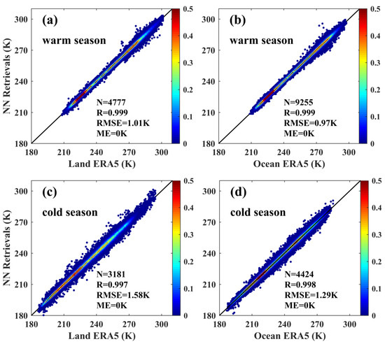
Figure 4.
Density scatter diagram of NNs-250 temperature retrievals. (a,b) Retrievals during warm season for temperature on land and ocean, respectively. (c,d) Retrievals during cold season for temperature on land and ocean, respectively.
Figure 5 is a density scatter diagram of relative humidity inversion between 100 and 1000 hPa (25 pressure layers). Compared with the temperature validation, the RH inversion density scatter diagram is more scattered, but most of the points are still concentrated on the straight line “Y = X”. Except for the warm season, whose coefficient on land is 0.93, the R of the other three models are all 0.94. The RMSE of RH retrievals on land and ocean in the warm season is 10.33% and 9.97%, respectively, and the RMSE of RH retrievals on land and ocean in the cold season is about 11%. The ME is less than zero. The RH retrievals are slightly smaller than ERA5 RH fields. Figure 3 also illustrates that relative humidity in the warm season is mostly less than 60%, and within 40% in the cold season.
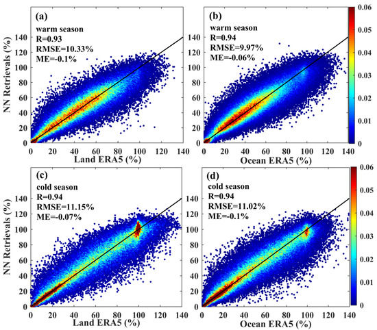
Figure 5.
Density scatter diagram of NNs-250 relative humidity retrievals. (a,b) Retrievals during warm season for relative humidity on land and ocean, respectively. (c,d) Retrievals during cold season for relative humidity on land and ocean, respectively.
4.2. Error Variation with Height Compared with ERA5
To further verify whether the retrieval performance of the NNs-250 built by HIRAS, MWTS, and MWHS observations proposed in this experiment have been improved compared with the original NNs-220 that were built only by HIRAS observations, we compared the RMSEs of temperatures retrieved from the two schemes. The results are shown in Figure 6a,c. The dotted lines and solid lines represent the RMSE of temperature profiles obtained from NNs-220 and NNs-250, respectively. It can be seen that the accuracy of NNs-250 has been improved compared with the original model NNs-220. Figure 6b,d are the RMSE of the temperature profile retrieved by NNs-250 minus NNs-220, which means the smaller the value, the more obvious the improvement. The two diagrams clearly illustrate the changes of improved accuracy with height. The retrieval performance of the troposphere below 600 hPa on land has improved more significantly than that in the ocean. The RMSE of temperature retrievals near 1000 hPa on land can be reduced by up to 0.45 K and 0.3 K in the cold and warm seasons, respectively. In the cold season, RMSE is also significantly reduced in stratosphere. After adding MW data in the ocean, temperature RMSE below 800 hPa is reduced by about 0.2 K, and the improvement effect is not much different in the warm and cold seasons. Due to strong radiative cooling, there is a near-surface temperature inversion in the polar region, and the frequency is higher and the temperature inversion layer is thicker in the cold season [48,49].
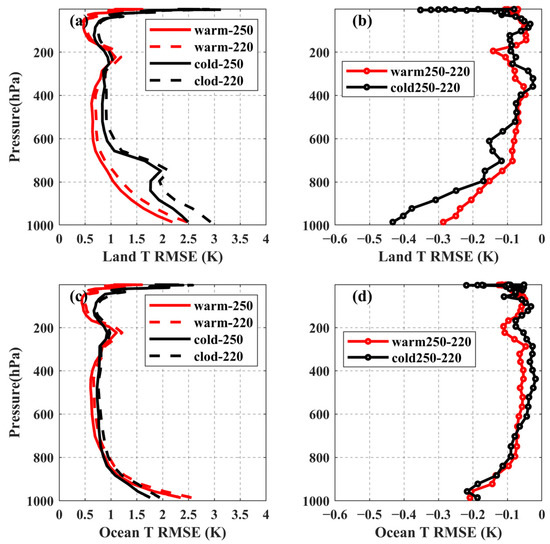
Figure 6.
Temperature profile retrieval RMSE, with respect to ERA5. (a,c) Comparisons of RMSE between NNs-250 and NNs-220, (b,d) profile retrieval RMSEs of NNs-250 minus that of NNs-220.
Figure 7 shows the comparison between the RMSE of RH profiles retrieved from NNs-250 and NNs-220. It can be seen that the inversion accuracy of the lower troposphere is also improved. The improvement in other levels is not obvious. The retrieval performance in the cold season is clearly improved on land, and the RMSE of the retrievals can be reduced by up to 1.5%. The accuracy of RH retrieval in the warm season on the ocean is improved more, and the RMSE can be reduced by up to 2%. Through the comparison of Figure 6 and Figure 7, it can be concluded that in order to obtain the high-precision temperature and RH profiles in the Arctic based on a NN algorithm, it is not enough to use FY-3D IR observations alone. Adding MW data as a supplement to IR data is a feasible way to improve the retrieval accuracy in the tropospheric bottom of the Arctic region from FY-3D satellite observations.
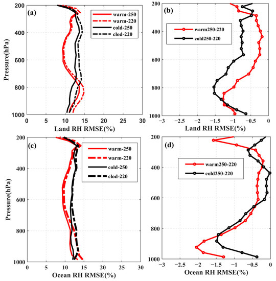
Figure 7.
Relative humidity profile retrieval RMSE, with respect to ERA5. (a,c) Comparisons of RMSE between NNs-250 and NNs-220, (b,d) profile retrieval RMSEs of NNs-250 minus that of NNs-220.
4.3. Retrieval Performance Sensitivity to Cloud Amount
The sensitivity of the improved NNs retrieval to cloud fraction over land in the cold season was evaluated in this study and the results are summarized herein. The retrieval RMSE of the improved NNs-250 under different cloud fraction was analyzed. The sensitivity of the improved NNs-250 retrieval to cloud fraction was compared with the NNs only built by HIRAS (NNs-220) data. The temperature and relative humidity results are shown in Figure 8 and Figure 9, respectively.
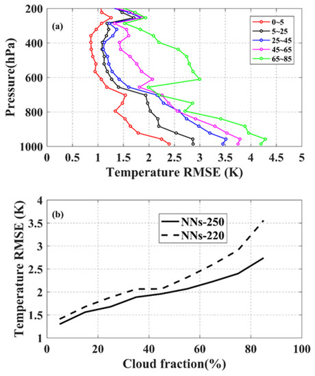
Figure 8.
Temperature RMSE over land between 200 and 1000 hPa in cold season. (a) Temperature profile RMSE of NNs-250 below 200 hPa, (b) cumulative temperature RMSE between 200 and 1000 hPa. Pixels are ranked in order of increasing cloudiness according to cloud fraction form FY-3D/MERSI-II L2 products.
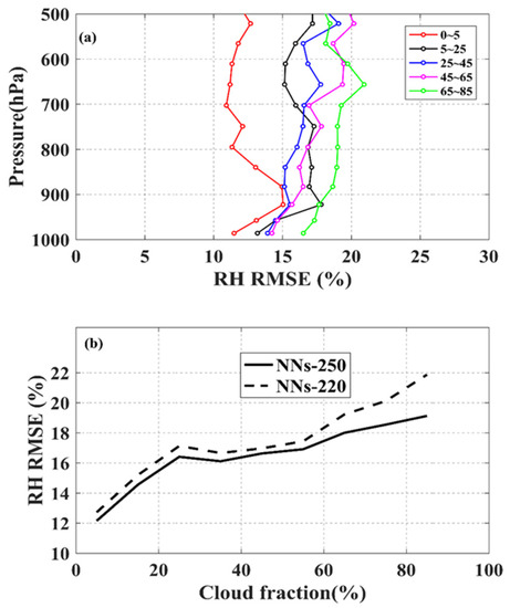
Figure 9.
Relative humidity RMSE over land between 500 and 1000 hPa in cold season. RH represents relative humidity. (a) RH profile RMSE of NN-250 below 500 hPa, (b) cumulative RH RMSE between 500 and 1000 hPa. Pixels are ranked in order of increasing cloudiness according to cloud fraction form FY-3D/MERSI-II L2 products.
From Figure 8a, which represents the temperature profiles’ RMSE over land between 200 and 1000 hPa under different cloud amounts, it can be observed that the RMSE of retrieved temperature profiles increased with the increased cloud amount, especially below 800 hPa. When the cloud fraction increases to 65–85%, temperature RMSE at about 1000 hPa can reach to 4.4 K, and the temperature RMSE between 300 and 600 hpa is also larger than other condition. Figure 8b shows the comparison of cumulated temperature RMSE between the improved NNs-250 and NNs-220. The cumulative temperature RMSE of NNs-220 is larger than that of NNs-250. The latter observation indicates that the performance of the improved NNs are superior to the NNs-220, and this advantage becomes more apparent as cloud cover increases.
Figure 9 is the analysis diagram of relative humidity below 500 Pha. The results are similar to those of retrieved temperature. When the cloud amount is less than 5%, the error of relative humidity retrieved from improved NNs-250 is the smallest, and when the cloud amount is more than 65%, the error of relative humidity inversion increases. Although RMSE of humidity profiles between 500 and 1000 hPa increases with the increase in cloud coverage, it can still remain less than 20%. In addition, the improved NNs-250 relative humidity retrievals are also less sensitive than NNs-220 to cloud fraction.
5. Retrieval Performance as Compared with Radiosonde Observations
Radiosonde observations were used to further evaluate the inversion performance. The accuracy verification results are shown in Figure 10. The samples for temperature and relative humidity obtained on the land in the warm season were 1511 and 1510, respectively. The samples for temperature and relative humidity obtained on the land in the cold season were 422 and 426, respectively. The accuracy of the temperature profile retrieved from NNs-250 was also improved in the middle and low troposphere compared with the NNs-220. The overall RMSE below 600 hPa was calculated, and the results are shown in Figure 8. Compared with NNs-220, the RMSE of temperatures below 600 hPa in the warm and cold seasons was reduced by about 0.1 K and 0.3 K, respectively. The accuracy improvement was more obvious in the cold season, and temperature RMSE can be reduced by up to 0.8 K. Similarly, the relative humidity retrieval accuracy improved significantly in the cold season, with an improvement of about 2%. The RMSE of retrieved profiles with respect to RAOBs is different from ERA5, which is related to the deviation between the two data themselves [50], but it can still be proved that it is feasible to use MW data as a supplement to infrared hyperspectral data to improve the accuracy of tropospheric inversion.
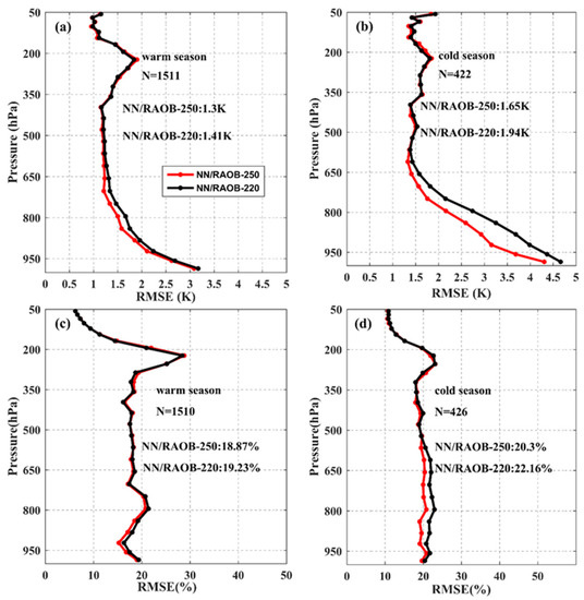
Figure 10.
Profile retrieval RMSEs, with respect to RAOBs. (Red lines and black lines represent RMSE of NNs-250 and NNs-220, respectively. (a,b) Temperature RMSE on warm and cold season, respectively, (c,d) relative humidity RMSE on warm and cold season, respectively. RMSE marked in the figure is mean errors from 50 to 1000 hPa.).
6. Comparison between NNs-250 Retrievals and Satellite Products
6.1. Compared with FY-3D/VASS L2
To evaluate the performance of NNs-250 proposed in this study, the predicted products of NNs-250 were compared with FY-3D/VASS L2 products in the cold season (from November 2019 to April 2020, using the same reference: ERA5). The samples obtained for temperature validation were 196 and 464 (out of testing data) on land and ocean, respectively. The samples obtained for relative humidity validation were 196 and 395 (out of testing data) on land and ocean, respectively. The results are shown in Figure 11 and Figure 12.
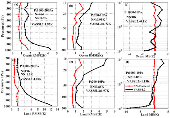
Figure 11.
Comparison of temperature between FY-3D/VASSL2 products and NNs-250 retrievals versus ERA5. (a–c) The results on ocean, (d–f) the results on land. The dotted line represents the comparison between the retrievals from NNs-250 and ERA5; the black solid line represents comparison between VASS products and the ERA5.
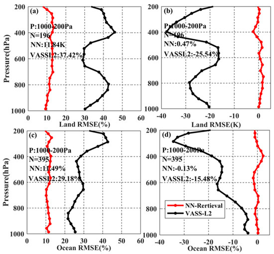
Figure 12.
Comparison of RH accuracy between FY-3D/VASSL2 products and NNs-250 retrievals versus ERA5. (a,b) The results on land. (c,d) The results in the ocean. The red dotted line represents the comparison between the retrievals fromNNs-250 and ERA5; the black solid line represents the comparison between VASS products and ERA5.
In Figure 11, the black line represents the RMSE of VASS products, and it illustrates that the accuracy needs to be urgently improved. This is reasonable due to the fact that only areas within 60° north–south latitude were included in the operational algorithm. RMSE of FY-3D/VASS L2 products is consistent with that of temperature retrieved from NNs. In the lower troposphere, the retrieval performance is poor, and the temperature inversion accuracy increases with the height. The first column clearly shows the comparison of tropospheric accuracy. The accuracy of the NNs-250 temperature retrievals has been significantly improved. The RMSE of NNs-250 retrievals and FY-3D/VASS products from 200 to 1000 hPa on land are 1.2 K and 4.07 K; the accuracy improved 2.95 K. The RMSE of NNs-250 retrievals and FY-3D/VASS products from 200 to 1000 hPa in the ocean are 0.9 K and 1.92 K; the accuracy improved 1.02 K. The middle column also illustrates that the performance of NNs-250 improved compared with VASS products in stratosphere. The right column shows that the temperature of VASS L2 product is lower than that of ERA5 in the troposphere as a whole, and larger in stratosphere. The ME of temperature retrieved by NNs-250 is about 0 K.
Figure 12 summarizes the RH comparison results. The accuracy of the RH profile retrieved from NNs proposed in this study has been significantly improved compared with the FY-3D/VASS L2 product. The RMSE of the RH from 200 to 1000 pHa on land decreased from 37.42 to 11.84%. The RMSE of RH reduced from 29.18 to 11.49% in the ocean. The FY-3D/VASS L2 relative humidity product is smaller than that of ERA5 in troposphere. The ME of RH inversion by NNs-250 is less than 1%.
6.2. Compared with Aqua/AIRS L2
In order to further prove the feasibility of the method proposed in this study, the accuracy of the inversion results were also compared with Aqua/AIRS L2 products (using the same reference: ERA5). The samples obtained for temperature validation were 255 and 1164 (out of testing data) on land and ocean, respectively; the samples obtained for relative humidity validation were 294 and 1165 (out of testing data) on land and ocean, respectively. The comparison results are shown in Figure 10 and Figure 11, respectively.
Figure 13 clearly reveals that the RMSE of temperature retrieved by NNs-250 is consistent with that of AIRS L2 temperature products on ocean and land. The first column clearly shows that the accuracy of the temperature retrieved by NNs-250 is equivalent to that of AIRS products in the middle and high troposphere, but the retrieval performance of NNs-250 is better than that of AIRS products below 800 hPa. NNs-250 has obvious advantages compared with AIRS products in the upper stratosphere. Figure 13c, f shows that ME of AIRS L2 (AIRS L2 temperature products minus ERA5 temperature) is less than 0 K, which demonstrates that AIRS L2 temperature products are generally lower than ERA5, and this phenomenon is more obvious in the stratosphere.
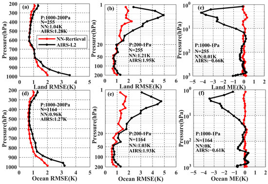
Figure 13.
Accuracy comparisons between Aqua/AIRS temperature products and NNs-250 retrievals versus ERA5. (a–c) The results on land. (d–f) The results in the ocean. The red dotted line represents the comparison between the retrievals from NNs-250 and ERA5; the black solid line represents comparison between AIRS products and the ERA5.
Figure 14 is the comparison of relative humidity results. Considering that AIRS relative humidity products are mostly filled values below 950 hPa and the inversion pressure layer is 50 hPa, the accuracy of relative humidity was compared between 50 and 900 hPa. The RMSE of RH profiles retrieved by NNs-250 is also consistent with AIRS products, but the performance of NNs-250 was better than that of AIRS products on the whole. The RMSE of RH from 50 to 950 hPa was been reduced by 2.8% and 4.2%, respectively. The results also reveal AIRS RH products are about 15% smaller than ERA5 at about 250 hPa.
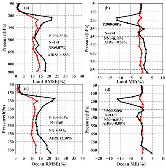
Figure 14.
Accuracy comparisons between Aqua/AIRS L2 relative humidity products and NNs-250 retrievals versus ERA5. (a,b) The results on land, (c,d) the results in the ocean. The red dotted line represents the comparison between the retrievals from NNs-250 and ERA5; the black solid line represents the comparison between AIRS products and ERA5.
7. Discussion
The present study has clearly established a dataset especially suitable for retrieving temperature and relative humidity profiles under clear sky conditions in the Arctic, and carried out the research of a neural network retrieval algorithm. In the proposed technique herein, we not only optimized the retrieval results from the NN algorithm itself, but also added MW data as a supplement into IR hyperspectral data to improve the inversion accuracy in the middle and lower troposphere. The results showed that the accuracy in the lower troposphere is improved both compared with the same method but just using IR observations, and compared with FY3D/VASS secondary products.
The study demonstrated the potential of the NN algorithm proposed herein in retrieving atmospheric temperature and relative humidity profiles under clear sky condition in the Arctic. Furthermore, adding MW measurement data to the infrared hyperspectral data can significantly improve the accuracy of retrieving middle and low troposphere profiles form FY-3D data. The method proposed herein allows temperature and relative humidity profiles to be obtained with improved accuracy, avoiding at the same time the complicated calculation process required by other analogous techniques. A key advantage of our proposed scheme is that it only needs Fengyun-3D/VASS observations as input of neural networks (established in advance) to capture temperature and relative humidity profiles synchronized with the satellite.
Although, compared with only using IR hyperspectral data, the accuracy of NNs built by adding MW observation data has been greatly improved in the middle and low troposphere, errors of NNs still come from the following three aspects. First of all, the setting of the algorithm parameters affect the accuracy of NNs, such as the number of hidden layer nodes. Although we have referred to the empirical formula and performed lots of experiments to find the optimal number, this may still not be the optimal value of NNs. Second, energy exchange between the surface and the lower atmosphere can affect the dynamic and thermal properties of the lower atmosphere. Furthermore, the strong radiative cooling of the surface in the Arctic region has caused the temperature inversion in lower atmospheres. These factors lead to a more complicated relationship between the atmospheric parameters and brightness temperature observed by satellites, which is currently unable to be solved by neural networks. Last but not least, the terrain is more complex, with large topographic heterogeneity and elevation differences over the Arctic region; the inversion accuracy of land is worse than that of the ocean.
8. Conclusions
In this study, a new technique based on the NN algorithm was proposed for improving the accuracy of retrieving the atmospheric parameters in the Arctic region (north of 60°N) under clear sky from FengYun-3D/VASS observations. Only these observations are needed as the NNs-250 input; the proposed technique allows obtaining more accurate temperature and RH profiles synchronized with the satellite time. ERA5 and radiosonde data independent of the training set were used to evaluate the performance of the advanced NNs. Furthermore, our retrievals were also compared with satellite L2 products including FengYun-3D/VASS L2 and Aqua/AIRS L2 products. The key study findings can be summarized as follows:
- Compared with NNs-220 built only by HIRAS data, the improved NNs-250 built by IR and MW measurements has a significant improvement in the inversion accuracy of atmospheric temperature at the bottom of the troposphere. The improvement of inversion accuracy is better in the cold season on land. Compared with ERA5 on land, the temperature RMSE of NNs-250 can be reduced by up to 0.45 K and 0.3 K in the cold and warm seasons, respectively. Compared with RAOBs on land, the temperature RMSE of NNs-250 can be reduced by up to 0.5 K in the cold season. The RH inversion accuracy has also been improved overall, but the improved accuracy is not as high as the temperature.
- Compared with the accuracy of FY-3D/VASS L2 products in the cold season, the RMSE of temperature in troposphere on the land and the ocean increased by 2.97 K and 1.02 K, respectively, and the RH increased by 25.58% and 17.69%. Compared with AIRS L2 products, the temperature on land and ocean in troposphere increased by 0.24 K and 0.3 K, respectively, and the relative humidity below 50 hPa increased by 2.8% and 4.2%, respectively.
- By comparing the influence of cloud coverage on the retrieval accuracy of NNs-250 with NNs-220, it is found that with the increase in cloud coverage, the retrieval accuracy of NNs-220 and NNs-250 both decrease, but NNs-220 decreases more significantly, which means that the sensitivity of the NNs-250 proposed in this study to cloud cover is weaker than that of NNs-220 and has better and more stable retrieval performance.
All in all, clouds will inevitably exist in the selected clear sky pixels due to the inaccuracy of MERSI L2 cloud products, which leads to the low retrieval accuracy form FY-3D/HIRAS observation under clear sky conditions, especially in the cold season with more clouds. The problem has been solved in this study after adding MW measurement observations from the same platform to FY-3D/HIRAS observations, as the lower resolution microwave measurements have far less sensitivity to clouds. Thus, the combination of IR and microwave observations (NNs-250) effectively improve the retrieval performance in middle and low troposphere in the Arctic, as this method can not only make up for the shortcoming of IR channels (NNs-220), but also improve the stability of retrieval performance when there are clouds in HIRAS’S FOV. Atmospheric profiles retrieved from NNs-250 are synchronized with the FY-3D; this can not only make up for the latency of ERA5, but also improve spatial and temporal resolution compared with RAOBs in the Arctic. Compared with the traditional statistical retrieval methods, such as eigenvector regression algorithm, the NN method proposed in this study has higher accuracy, compared with a physically based retrieval method, this method avoids complex and time-consuming calculation processes. Therefore, our method has great prospects in the precision and practicability of potential operationalization. The present study does not only provide basic data for meteorological and climate research in the Arctic region, but also provides technical support for broadening FY-3D’s operational implementation range from 60O N to the Arctic region and guaranteeing the quantitative application of satellite remote sensing data. Although, the NNs-250 cannot be used in the operationalization now, because surface information still did not include surface elevation information, surface temperature, etc. This seems the biggest influencing factor affecting the accuracy of near-surface retrieval by our proposed method herein. Further work in improving the proposed scheme can be directed towards exploring the added value of non-satellite observation factors in addition to satellite observations, which is an area of future research.
Author Contributions
Conceptualization, J.H., J.W. and Y.B.; methodology, J.H., Y.B., J.L., H.L. and G.P.P.; software, J.H.; validation, J.L., Q.L. and H.L.; formal analysis, Y.B. and G.P.P.; investigation, J.H.; resources, J.L. and H.L.; data curation, J.H.; writing—original draft preparation, J.H., Y.B. and H.L.; writing—review and editing, J.H., G.P.P., F.W. and Y.B.; supervision, Y.B. and H.Z.; project administration, J.L. and H.L.; funding acquisition, Y.B. and J.L. All authors have read and agreed to the published version of the manuscript.
Funding
This study was funded by the Joint Fund for Meteorology, the National Natural Science Foundation of China and the China Meteorological Administration (U2242212), the National Key Research and Development Program of China (2021YFC2803300, 2021YFC2803303), and the Shanghai Aerospace Science and Technology Innovation Fund (SAST2021-032). GPP’s participation in the research study was financially supported by the project “EO-PERSIST” European Union’s Horizon Europe Research and Innovation program HORIZON-MSCA-2021-SE-01-01 under grant agreement N° 101086386.
Data Availability Statement
All data generated or analyzed during this paper are included in this article. All the data used in this study can be obtained from the websites for free. The FY-3D observations used can be obtained from the National Satellite Meteorological Center. Atmospheric profile data can be obtained from ECMWF and the University of Wyoming.
Acknowledgments
The numerical calculations in this paper were performed on the supercomputing system in the Supercomputing Center of Nanjing University of Information Science & Technology. We thank the National Satellite Meteorological Center for providing the satellite data, which were obtained on this website (http://satellite.nsmc.org.cn/PortalSite/Data/Satellite.aspx, accessed on 30 April 2020), and the ECMWF for providing ERA5 reanalysis data used here (https://cds.climate.copernicus.eu/#!/search?text=ERA5&type=dataset, accessed on 30 April 2020). Last but not least, we appreciate the sounding data that was provided by the University of Wyoming, and this data can be archived online (http://weather.uwyo.edu/upperair/sounding.html, accessed on 30 April 2020).
Conflicts of Interest
The authors declare no conflict of interest.
References
- Kay, J.E.; Ecuyer, T.L.; Chepfer, H.; Loeb, N.; Morrison, A.; Cesana, G. Recent Advances in Arctic Cloud and Climate Research. Curr. Clim. Chang. Rep. 2016, 2, 159–169. [Google Scholar] [CrossRef]
- Zhang, B.; Li, F.; Sang, H.; Cressie, N. Inferring Changes in Arctic Sea Ice through a Spatio-Temporal Logistic Autoregression Fitted to Remote-Sensing Data. Remote Sens. 2022, 14, 5995. [Google Scholar] [CrossRef]
- Xiao, F.; Zhang, S.; Li, J.; Geng, T.; Xuan, Y.; Li, F. Arctic sea ice thickness variations from CryoSat-2 satelliate altimetry data. Sci. China Earth Sci. 2021, 64, 1080–1089. [Google Scholar]
- Hoffman, J.P.; Ackerman, S.A.; Liu, Y.; Key, J.R. A 20-Year Climatology of Sea Ice Leads Detected in Infrared Satellite Imagery Using a Convolutional Neural Network. Remote Sens. 2022, 14, 5763. [Google Scholar] [CrossRef]
- Mengis, N.; Martin, T.; Keller, D.P.; Oschlies, A. Assessing climate impacts and risks of ocean albedo modification in the Arctic. J. Geophys. Res. Ocean. 2016, 121, 3044–3057. [Google Scholar] [CrossRef]
- Xie, Q.; Chen, H. Research progress of anti-icing/deicing technologies for polar ships and offshore platforms. Chin. J. Ship Res. 2017, 12, 45–53. [Google Scholar]
- Battisti, L.; Brighenti, A. Sea ice and icing risk for offshore wind turbines. In Proceedings of the OWEMES, Civitavecchia, Italy, 20–22 April 2006. [Google Scholar]
- Wang, Y.; Zhang, R.; Wang, Z.; Zhu, Y. Integrated Assessment Model of Arctic Routes with Climate Change. Ocean. Dev. Manag. 2017, 34, 118–124. [Google Scholar]
- Jiang, S.; Yang, Q.H.; Liang, Y.Q.; Teng, J.H.; Lin, Z. Sea Ice And Weather Forecasting Information for Arctic Sea Routes: A Synthetic Analysis. Chin. J. Polar Res. 2017, 29, 399–413. [Google Scholar]
- Liu, D.; Ma, Y.; Wang, C.; Xing, W.; Meng, X. Developments of Arctic Passage Resources Under Global Climate Change. China Popul. Resour. Environ. 2015, 25, 6–9. [Google Scholar]
- Gui, K.; Che, H.; Chen, Q.; Zeng, Z.; Liu, H.; Wang, Y.; Zheng, Y.; Sun, T.; Liao, T.; Wang, H.; et al. Evaluation of radiosonde, MODIS-NIR-Clear, and AERONET precipitable water vapor using IGS ground-based GPS measurements over China. Atmos. Res. 2017, 197, 461–473. [Google Scholar] [CrossRef]
- Yao, Z.-G.; Hong, J.; Cui, X.-D.; Zhao, Z.-L. A Neural Network Based Single Footprint Temperature Retrieval for Atmospheric Infrared Sounder Measurements and Its Application to Study on Stratospheric Gravity Wave. J. Trop. Meteorol. 2022, 28, 82–94. [Google Scholar]
- Zhang, C.; Gu, M.; Hu, Y.; Huang, P.; Yang, T.; Huang, S. A Study on the Retrieval of Temperature and Humidity Profiles Based on FY-3D/HIRAS Infrared Hyperspectral Data. Remote Sens. 2021, 13, 2157. [Google Scholar] [CrossRef]
- Aires, F.; Pellet, V. Estimating Retrieval Errors From Neural Network Inversion Schemes—Application to the Retrieval of Temperature Profiles From IASI. IEEE Trans. Geosci. Remote Sens. 2021, 59, 6386–6396. [Google Scholar] [CrossRef]
- He, Q.; Wang, Z. Application of the Deep Neural Network in Retrieving the Microwave Humidity and Temperature Sounder Onboard the Feng-Yun-3 Satellite. Sensors 2021, 21, 4673. [Google Scholar] [CrossRef]
- Feng, J.; Qin, X.; Wu, C.; Zhang, P.; Yang, L.; Shen, X. Improving typhoon predictions by assimilating the retrieval of atmospheric temperature profiles from the FengYun-4A’s Geostationary Interferometric Infrared Sounder (GIIRS). Atmos. Res. 2022, 280, 106391. [Google Scholar] [CrossRef]
- Xue, Q.; Guan, L.; Shi, X. One-Dimensional Variational Retrieval of Temperature and Humidity Profiles from the FY4A GIIRS. Adv. Atmos. Sci. 2022, 39, 471–486. [Google Scholar] [CrossRef]
- König, N.; Wetzel, G.; Höpfner, M.; Friedl-vallon, F.; Johansson, S.; Kleinert, A.; Schneider, M.; Ertl, B.; Ungermann, J. Retrieval of Water Vapour Profiles from GLORIA Nadir Observations. Remote Sens. 2021, 13, 3675. [Google Scholar] [CrossRef]
- Giri, R.K.; Yadav, R.; Ranalkar, M.; Singh, V. Validation of INSAT-3DR sounder retrieved temperature frofile with GPS radiosonde and AIRS observations. Adv. Space Res. 2022, 69, 1100–1115. [Google Scholar] [CrossRef]
- Hu, J.; Bao, Y.; Liu, J.; Liu, H.; Petropoulos, G.P.; Katsafados, P.; Zhu, L.; Cai, X. Temperature and Relative Humidity Profile Retrieval from Fengyun-3D/HIRAS in the Arctic Region. Remote Sens. 2021, 13, 1884. [Google Scholar] [CrossRef]
- Chen, Y. Research on Cloud Detection Method under Arctic Ice Environment Based on FY-3D MERSI-II. Geospat. Inf. 2020, 18, 10–15. [Google Scholar]
- Qu, J.; Yang, J.; Wang, Y. Global Clear-Sky Data Synthesis Technology Based on FY-3D MERSI-II Instrument. Meteorol. Sci. Technol. 2019, 47, 539–545. [Google Scholar]
- Eastman, R.; Warren, S.G. Interannual variations of arctic cloud types in relation to sea ice. J. Clim. 2010, 23, 4216–4232. [Google Scholar] [CrossRef]
- Wang, X.; Huang, F.; Wang, H. Seesaw Pattern of Arctic Cloud Cover Trend in Spring and Its Cloud Feedback Effect for Arctic Amplification. Period. Ocean Unive. China 2020, 50, 10–17. [Google Scholar]
- Hu, H.; Weng, F. Progress in Satellite Microwave Remote Sensing of Atmospheric Temperature and Moisture Profiles and Their Applications. Adv. Met S&T 2021, 11, 40–47. [Google Scholar]
- Milstein, A.B.; Blackwell, W.J. Neural network temperature and moisture retrieval algorithm validation for AIRS/AMSU and CrIS/ATMS. J. Geophys. Res. Atmos. 2015, 121, 1414–1430. [Google Scholar] [CrossRef]
- Zhang, Y.; Zhang, S.; Wang, Z.; Jiang, J.; Li, J. Technology Development of Atmospheric Humidity Sounding of FY-3 Satellite. Shanghai Aerosp. 2017, 34, 52–61. [Google Scholar] [CrossRef]
- Hou, X.; Han, Y.; Hu, X.; Weng, F. Verification of Fengyun-3D MWTS and MWHS Calibration Accuracy Using GPS Radio Occultation Data. J. Meteorol. Res. 2019, 33, 695–704. [Google Scholar] [CrossRef]
- Yang, J.; Zhang, P.; Lu, N.; Yang, Z.; Shi, J.; Dong, C. Improvements on global meteorological observations from the current Fengyun 3 satellites and beyond. Int. J. Digit. Earth 2012, 5, 251–265. [Google Scholar] [CrossRef]
- Wu, C.; Qi, C.; Hu, X.; Gu, M.; Yang, T.; Xu, H.; Lee, L.; Yang, Z.; Zhang, P. FY-3D HIRAS Radiometric Calibration and Accuracy Assessment. IEEE Trans. Geosci. Remote Sens. 2020, 58, 3965–3976. [Google Scholar] [CrossRef]
- Wang, X.; Zou, X. Quality Assessments of Chinese FengYun-3B Microwave Temperature. IEEE Trans. Geosci. Remote Sens. 2012, 50, 4875–4884. [Google Scholar] [CrossRef]
- Niu, Z.; Zhang, L.; Dong, P.; Weng, F.; Huang, W. Impact of Assimilating FY-3D MWTS-2 Upper Air Sounding Data on Forecasting Typhoon Lekima (2019). Remote Sens. 2021, 13, 1841. [Google Scholar] [CrossRef]
- Lin, K.; Xiao, S.; Zhou, A.; Liu, H. Experimental study on long-term performance of monopile-supported wind turbines (MWTs) in sand by using wind tunnel. Renew. Energy 2020, 159, 1199–1214. [Google Scholar] [CrossRef]
- Han, Y.; Yang, J.; Hu, H.; Dong, P. Retrieval of Oceanic Total Precipitable Water Vapor and Cloud Liquid Water from Fengyun-3D Microwave Sounding Instruments. J. Meteorol. Res. 2021, 35, 371–383. [Google Scholar] [CrossRef]
- Space, N. Assimilation of FY-3D MWHS-2 Radiances with WRF Hybrid-3DVAR System for the Forecast of Heavy Rainfall Evolution Associated with Typhoon Ampil. Mon. Weather. Rev. 2021, 149, 1419–1437. [Google Scholar] [CrossRef]
- Vessey, A.F.; Hodges, K.I.; Shaffrey, L.C.; Day, J.J. An inter-comparison of Arctic synoptic scale storms between four global reanalysis datasets. Clim. Dyn. 2020, 54, 2777–2795. [Google Scholar] [CrossRef]
- Christensen, T.; Knudsen, B.M.; Pommereau, J.; Letrenne, G.; Hertzog, A. Evaluation of ECMWF ERA-40 temperature and wind in the lower tropical stratosphere since 1988 from past long-duration balloon measurements. Atmos. Chem. Phys. 2007, 7, 3423–3450. [Google Scholar] [CrossRef]
- Reanalyses, N. Surface Heat Fluxes over the Northern Arabian Gulf and the Northern Red Sea: Evaluation of ECMWF-ERA5 and NASA-MERRA2 reanalyses. Atmosphere 2019, 10, 504. [Google Scholar] [CrossRef]
- Wang, L.; Tremblay, D.; Zhang, B.; Han, Y. Fast and accurate collocation of the visible infrared imaging radiometer suite measurements with Cross-track Infrared Sounder. Remote Sens. 2016, 8, 76. [Google Scholar] [CrossRef]
- Chen, Y.L. A method and its retrieval application for collocating the FY-3 microwave and VIS/IR data. Sci. China Press 2016, 61, 2939–2951. [Google Scholar] [CrossRef]
- Krasnopolsky, V.M. Neural network emulations for complex multidimensional geophysical mappings: Applications of neural network techniques to atmospheric and oceanic satellite retrievals and numerical modeling. Rev. Geophys. 2007, 45, 1–34. [Google Scholar] [CrossRef]
- Hecht-nielsen, R. Theory of the Backpropagation Neural Network. In Proceedings of the International 1989 Joint Conference on Neural Networks, Washington, DC, USA, 1989; pp. 593–605. [Google Scholar]
- Cai, X.; Bao, Y.; Petropoulos, G.P.; Lu, F.; Lu, Q.; Zhu, L.; Wu, Y. Temperature and humidity profile retrieval from FY4-GIIRS hyperspectral data using artificial neural networks. Remote Sens. 2020, 12, 1872. [Google Scholar] [CrossRef]
- Bao, Y.; Cai, X.; Qian, C.; Min, J.; Lu, Q.; Zuo, Q. 0–10 km temperature and humidity profiles retrieval from ground-based microwave radiometer. J. Trop. Meteorol. 2018, 24, 223–252. [Google Scholar]
- Sai Gowtam, V.; Tulasi Ram, S. An Artificial Neural Network-Based Ionospheric Model to Predict NmF2 and hmF2 Using Long-Term Data Set of FORMOSAT-3/COSMIC Radio Occultation Observations: Preliminary Results. J. Geophys. Res. Space Phys. 2017, 122, 11743–11755. [Google Scholar] [CrossRef]
- Zheng, G.; Yang, J.; Li, X.; Zhou, L.; Ren, L.; Chen, P.; Zhang, H.; Lou, X. Using artificial neural network ensembles with crogging resampling technique to retrieve sea surface temperature from HY-2A scanning microwave radiometer data. IEEE Trans. Geosci. Remote Sens. 2019, 57, 985–1000. [Google Scholar] [CrossRef]
- Jiao, B.; Ye, M. Determination of Hidden Unit Number in a BP Neural Network. J. Shanghai Dianji Univ. 2013, 16, 113–117. [Google Scholar]
- Cheng, G.; Gao, Z.; Zheng, Y.; Dai, C.; Zhou, M. A Study on Low-level Jets and Temperature Inversion over the Arctic Ocean by using SHEBA Data. Clim. Environ. Res. 2013, 18, 23–31. (In Chinese) [Google Scholar] [CrossRef]
- Kahl, J.; Schnell, R. Low-Level Temperature Inversions of the Eurasian Arctic and Comparisons with Soviet Drifting Station Data. J. Clim. 1992, 5, 615–629. [Google Scholar]
- Keernik, H.; Jakobson, E. Evaluating reanalyses performance in the Baltic Sea region by using assimilated radiosonde data. Int. J. Climatol. 2018, 38, 1820–1832. [Google Scholar] [CrossRef]
Disclaimer/Publisher’s Note: The statements, opinions and data contained in all publications are solely those of the individual author(s) and contributor(s) and not of MDPI and/or the editor(s). MDPI and/or the editor(s) disclaim responsibility for any injury to people or property resulting from any ideas, methods, instructions or products referred to in the content. |
© 2023 by the authors. Licensee MDPI, Basel, Switzerland. This article is an open access article distributed under the terms and conditions of the Creative Commons Attribution (CC BY) license (https://creativecommons.org/licenses/by/4.0/).