Radiometric and Polarimetric Quality Validation of Gaofen-3 over a Five-Year Operation Period

Abstract

GaoFen-3 was the first Chinese civilian C-band synthetic aperture radar (SAR) satellite, launched in August 2016. The need for monitoring the satellite’s image quality has been boosted by its widespread applications in various fields. The efficient and scientific assessment of the system’s radiometric and polarimetric performance has been essential in its more than five years of service. The authors collected 90 images of the Inner Mongolia calibration site, 888 images of the Amazon rainforest, and 39,929 images of the Chinese mainland from 2017 to 2021. This was achieved whilst covering the leading imaging modes, such as the spotlight mode, stripmap mode, ultra-fine mode, wave imaging mode, etc. In this study, we derive a framework that incorporates the man-made corner reflectors (CRs) in Mongolia, the traditional Amazon rainforest datasets, and even the long-strip data in the Chinese mainland (known as CRAS) for the purposes of GaoFen-3 radiometric quality analysis and polarimetric validation over its five years of operation. Polarimetric calibration without recourse to the CRs is utilized to measure the polarimetric distortions regardless of the region, and thus requires a higher calibration accuracy for the GaoFen-3 polarimetric monitoring task. Consequently, the modified Quegan method is developed by relaxing the target azimuth symmetry constraint with the Amazon forest datasets. The experiments based on the CRAS demonstrate that the main radiometric characteristics could reach the international level, with an estimated noise-equivalent sigma zero of approximately −30 dB, a radiometric resolution that is better than 2.9 dB, and a single-imagery relative radiation accuracy that is better than 0.51 dB. For polarimetric validation, the modified Quegan method was utilized to measure the crosstalk for quad-pol products to ensure that it was than −40 dB. Meanwhile, non-negligible channel imbalance errors were found in the QPSII and WAV modes, and they were effectively well-calibrated with strip estimators to satisfy the system design.

1. Introduction

In recent years, countries around the world have been devoted to studying a series of satellites to develop space remote sensing businesses. The polarimetric synthetic aperture radar (PolSAR) system is the focus of research, owing to its capability of effectively penetrating clouds, its timely monitoring of day and night, and its intelligent transmitting and receiving of electromagnetic waves with fully polarimetric properties [1,2]. Several successful commercial PolSAR systems, such as the Canadian Radarsat-2, German TerraSAR, Japanese PALSAR, PALSAR2, and others, are well known. Although the Chinese GaoFen-3 mission started late, the products have been largely applied in target detection, classification, quantitative retrieval, and many other fields, benefiting from the close attention of the remote sensing community [3,4,5,6,7].

The C-band GaoFen-3 is designed with 12 imaging modes for environmental protection, emergency calling, periodic monitoring, and other purposes [8]. The spotlight (SL) mode and the ultra-fine strip (UFS) mode produce products with single polarization (HH/VV or DH/DV). The system transmits horizontal or vertical waves and receives the returned waves with the same polarization. Owing to the unique imaging mechanism, the SL mode can obtain images with a spatial resolution of 1 m. The pulse repetition frequency (PRF) of the UFS is lower, and due to the increasing spatial sampling in the azimuth direction, its imaging extent is more extensive than that of SL, while the spatial resolution is slightly lost. Dual-polarization products (HH-HV/VV-VH) can be acquired using the fine strip (FSI, FSII) modes and the standard strip (SS) mode. The dual products can help to balance the needs of spatial resolution and imaging extent, as well as being applicable for large-scale mapping or crop growth monitoring. The popular quad-polarization (HH-HV-VH-VV) products are produced using the normal quad-pol strip (QPSI, QPSII) modes and wave (WAV) mode. While working in the quad-pol mode, the system alternately transmits the H-pol or V-pol wave. Compared with QPSI, the WAV mode is designed to produce the products in discontinuous operation over a nominal mapping area of 5 km $\times$ 5 km. The number of QPSII datasets is relatively low, but it could still allow us to observe the ground targets with full polarization as an alternative. In this study, other imaging modes that may not be commonly used are not be mentioned in detail.

Since the GaoFen-3 experimental operation, the Institute of Electronics of the Chinese Academy of Sciences has performed ground validation yearly at the ground calibration site in Inner Mongolia, northern China [9]. By using the corner reflectors (CRs) deployed in the Inner Mongolia site, experts can further enhance their system quality evaluation work and initiate novel improvements. In 2018, Chen et al. [10] measured five radiation parameters, including the main lobe width and the side lode ratio, based on the impulse response of two trihedral CRs (TCR). In 2019, three years after the launch, Liang et al. [9] calibrated the quad-pol datasets with a combination of various CRs, including polarimetric active radar calibrators (PARCs), dihedral CRs (DCRs), and traditional TCRs. In 2020, Shi et al. [11] calculated the polarimetric distortion for early 2017 and 2018 QPSI products in Inner Mongolia and discovered that the co-pol channel imbalance phase level exceeded the ±10° design specification, with the radar internal calibration circuit failing to work at times; the phase error was eventually carefully calibrated with six strip observations rather than by using CRs. In recent years, polarimetric calibration and validation using natural targets or special artifacts has gradually become the strategy of many scholars, which has contributed to the flexible assessment of GaoFen-3’s system quality [12,13,14,15]. Furthermore, Shi et al. [16] fully estimated the noise equivalent sigma zero (NESZ) level, which was not stored in the header files in the QPSI and QPSII modes, using over 4000 collected images that were taken in the ocean.

The studies mentioned above attempted to analyze GaoFen-3’s system performance. However, further insights can be gleaned from the following aspects. First, most scholars have experimented with a single common imaging mode; as such, there is a lack of comprehensive assessment work on multiple modes. In general, the analysis was mainly focused on the QPSI mode; thus, users know little about the other useful imaging modes. UFS, FSI, FSII, and other modes are also widely applied, and it is of great importance to monitor the image quality during long-term missions. Second, previous studies, including analyses of radiation parameters or NESZ estimation, only discussed the specific characteristics needed to support radar applications. However, the details of GaoFen-3’s radiometric and polarimetric performance have not yet been jointly evaluated. Third, previous experiments on polarimetric quality have been conducted with the products acquired during the early stages of system operation. The results cannot be used as a guideline, particularly when the system has been through over half its life cycle. The system’s stabilization in the future needs further validation. Finally, to precisely calibrate the polarimetric distortions of GaoFen-3 worldwide, the traditional methods that do not rely on man-made CRs need to be improved. For example, Quegan’s [15] approach ignored the cross-pol channel observations for crosstalk estimation and dropped all second-order terms when expanding the calibration model, thereby resulting in insufficient crosstalk estimates. Ainsworth et al. [17] imposed the weakest target constraints, but the method was time-wasted and created the problem of dependent calculations for crosstalk ratios [18].

In this research, we perform a quality evaluation of the leading imaging modes of the GaoFen-3 system, including SL, UFS, FSI, FSII, SS, QPSI, QPSII, and WAV, by combining nine radiometric and polarimetric characteristics in time series and fully accounting for the sing-pol, dual-pol, and quad-pol products. We integrate the CRs, the traditional Amazon forest, and the long-strip measurements (known as CRAS) with 90 images from the Inner Mongolia calibration site, 888 images from the Amazon rainforest, and 39,929 images from the Chinese mainland that were collected from June 2017 to December 2021 in order to accurately assess GaoFen-3’s radiometric quality. For the polarimetric assessment in this research, we improve the traditional Quegan method and build the $\alpha$-preserving criterion to modify the solution of the calibration equations to explicitly incorporate the relaxing target azimuth symmetry constraint. This proposed approach aims to address the following two main defects of GaoFen-3’s polarimetric validation: (1) the accuracy of the original Quegan technique is in doubt when the system antenna subarrays are not highly isolated, since the cross-pol channel observations are ignored for simplifying the solutions to crosstalk sets; (2) previous efforts were made by Ainthworth et al. to iteratively solve the standard non-linear calibration equations [17], but the coupled calculation problem was still evident. With the help of the modified Quegan method, we effectively achieved system polarimetric calibration and validation over five years of operation.

The rest of this paper is organized as follows. In Section 2, the derived CRAS framework for evaluating the radiometric and polarimetric quality of GaoFen-3 is introduced. In Section 3, the radiometric assessment results are analyzed in detail. In Section 4, the polarimetric distortions are calibrated, and we compare the system quality with Radarsat-2 in Section 5. The conclusion and future work are presented in Section 6.

2. The Derived CRAS

In this section, we focus on nine radiometric and polarimetric characteristics and derive the time-series CRAS framework for the leading imaging modes. The procedure is shown in Figure 1, and detailed methods for GaoFen-3’s system quality evaluation are presented.

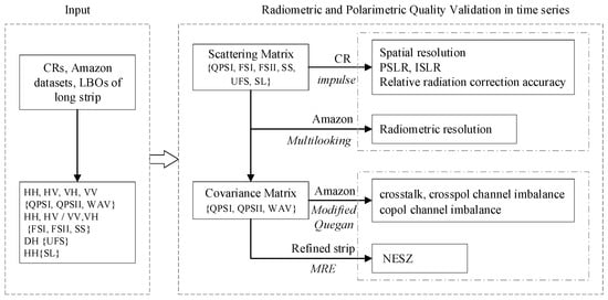
Figure 1. Procedure of the derived CRAS.

2.1. CR Response for System Quality

Man-made CRs are essential targets, whether they are for external calibration or for periodic system quality validation campaigns. On this basis, the Inner Mongolia calibration site is very helpful. Common PARCs, DCRs, and TCRs can usually be found in the GaoFen-3 products that were acquired during the summer season from 2017 to 2021, as shown in Figure 2. The true radar cross-section (RCS) can be calculated with the known radar wavelength and the CR size [19]. For an ideal TCR, the peak value of its RCS is given as follows:

$${\sigma }_{pq}^{TCR}=\frac{4\pi L^4}{3{\lambda }^2},$$

(1)

where L is the TCR leg length in meters (m) and $\lambda$ is the radar wavelength (in m). For GaoFen-3, the RCS of the TCRs deployed, as shown in Figure 2d, should be 34.9238 dB with a C-band wavelength of 0.056 m and a length of 1.235 m. This theoretical RCS is crucial for evaluating the system’s radiometric accuracy. Furthermore, the RCS of the CR samples in the time-series products can be measured, and the method will be given in the next part.

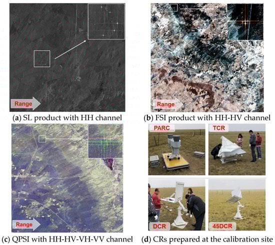
Figure 2. Examples of the GaoFen-3 single-pol, dual-pol, and quad-pol products with CR pixels acquired from the Mongolia calibration site on 17 October 2021, 6 September 2020, and 6 June 2017, respectively. (a) The intensity image of the SL mode is represented in decibels (dB); (b) a pseudo-RGB image, with the color combination of the HV, HV + VV, and HH channels of the FSI mode; (c) a PauliRGB image of the standard QPSI product; and (d) the PARC, TCR, DCR and 45°-rotated DCR (45DCR) devices at the Mongolia calibration site in September 2018 [11].

In addition to the peak RCS, the CR impulse is of great importance in terms of analyzing the radiation characteristics of radar patterns. The ideal CR response is presented similar to a sinc function, which helps to measure the critical parameters, including the impulse response width (IRW) that defines the system’s spatial resolution, as well as the sidelobe ratio that pertains to the image contrast [20]. In general, to expand and oversample the CR points in radar-returned signals, the necessary interpolation in the radar azimuth and range direction is implemented for the CR pixel and its surrounding samples via the Fourier transform.

(1) Spatial resolution is the measure of the smallest feature that can be distinguished by the SAR system when imaging the ground. The 3-dB IRW of the CR response is used to deduce the following practical system’s spatial resolution (in m):

$${\delta }_{sr}=L\cdot {\gamma }_{ps},$$

(2)

where$L$, expressed in pixel units, is the width of the CR response measured at 0.707 below the peak magnitude [20] and ${\gamma }_{ps}$ is the pixel spacing in the radar azimuth or range direction.

(2) PSLR is a useful parameter for assessing the influence of the background clutter surrounding the point target. For the recorded pulse, the main lobe refers to the central area gathering the most returned energy; the remainder of the pulse located on two sides of the main lobe and the one with a similar shape is collectively known as the side lobe. The ratio between the peak power value of the main lobe and that of its near side lobe is called PSLR (in dB), which is expressed as

$$PSLR=10lg\frac{P_{side}}{P_{main}},$$

(3)

where $P_{side}$ is the peak of the side lobe, and $P_{main}$ is the peak of the main lobe. In the standard sinc function, the PSLR is approximately −13 dB. The high radar PSLR in the azimuth and range direction will prevent the illuminated targets from being covered with the surrounding objects. For Gaofen-3, the design specification of PSLR is −20 dB [8].

(3) ISLR is the other measure used for background clutter over an area and plays an important role when imaging an evenly distributed weaker scene [21]. The ratio between the cumulative intensity of the main lobe and that of the remaining side lobes is defined as ISLR (in dB) as follows:

$$ISLR=10lg\left\{\frac{E_{total}-E_{main}}{E_{main}}\right\},$$

(4)

where $E_{main}$ is the integrated energy in the main lobe, and $E_{total}$ is that of the whole pulse. The main lobe amplitude is restricted by the pulse measurements between the two lowest values in the central records. In this study, ISLR refers to the one-dimensional estimator in the range and azimuth directions. For GaoFen-3, ISLR should be lower than −13 dB [8].

(4) Relative radiation correction accuracy is used to evaluate the radar’s radiometric stability and accuracy, and it is defined as the bias of the radar repeated measurements of the CR’s RCS. In the time-series products, the measured RCS of the CR pixels ${\sigma }_{CR}$ can be estimated using the integral method as follows [22]:

$$\begin{gathered} {\sigma }_{CR}=E_{CR}\cdot A \\ {E}_{CR}=\left(E_n-\left(\frac{N_{CR}}{N_{clt}}\right)*E_{clt}\right), \end{gathered}$$

(5)

where $E_{CR}$ is the CR’s energy calculated in a cross window, and A is the area of the resolution cell. In the square window centered on the CR, $E_n$ is the total energy, $E_{clt}$ is the integrated energy for four clutter quadrants, and $N_{CR}$ and $N_{clt}$ are the numbers of defined clutter samples and CR samples, respectively.

In the few seconds when imaging the calibration site, the relative radiation correction accuracy is calculated with the measured RCS of CRs as follows:

$$\Delta R=\sqrt{{{\displaystyle \sum }}_{i=1}^N\frac{\left({\sigma }_{CR}^i-{\stackrel{-}{\sigma }}_{CR}\right)}{N}},$$

(6)

where ${\sigma }_{CR}^i$ denotes the RCS of the i-th CR, ${\stackrel{-}{\sigma }}_{CR}$ is the average, and N is the number of CRs in one image.

2.2. Natural Observation for System Evaluation

(1) NESZ is an essential measure of the SAR system’s sensitivity to low backscattering areas [23]. As mentioned in Section 1, despite being a crucial system parameter, NESZ is not stored in the GaoFen-3 header files. In a previous study [3], estimation was mainly performed via the QPSI or QPSII beam. However, the time-series analysis of GaoFen-3’s NESZ level was not the main research focus, and the parameter has still, at present, not yet been provided. In this study, we identify the low backscattering objects (LBOs) in long-strip observations for a time-series NESZ assessment. It is recognized that the difference between the HV and VH channels in the well-calibrated image can be utilized to deduce the NESZ, and the minimum eigenvalue (ME) method is the most used estimator [24]. The method can be improved by combining the LBOs [16]. As the aim of the study is to evaluate time-series products, we simultaneously refine the NESZ of the long-strip products in the same orbit and beam code by day. First, the LBOs are distinguished in each image; then, the ME is utilized to generate ${{\rm N}}_{ME}\left(LBOs\right)$. For m products in a single orbit of long strips, we extract the noise level in the middle range of each of them, and then the noise result in its orbit is deduced via optional operation ${\rm E}\{\cdot \}$, i.e., minimum, median, or polynomial fitting. Finally, we present and analyze the time-series NESZ based on the refined long strip. The middle-range estimator (MRE) is represented by ${{\rm N}}_{MR}$ as follows:

$$\begin{gathered} {{\rm N}}_{ME}=10\mathit{lg}\left(\mathit{min}\left\{{\lambda }_1,{\lambda }_2,{\lambda }_3,{\lambda }_4\right\}\right) \\ {{\rm N}}_{MR}=10\mathit{lg}\left({\rm E}{\left\{{{\rm N}}_{ME}{\left(LBOs\right)}_1,{{\rm N}}_{ME}{\left(LBOs\right)}_2,\dots ,{{\rm N}}_{ME}{\left(LBOs\right)}_m\right\}}_{LS}\right). \end{gathered}$$

(7)

(2) Radiometric resolution is the radiometric indicator that describes the radar’s ability to discriminate targets with similar reflection properties [25]. It is a crucial parameter for the quantitative interpretation of radar images. For the returned signal in a resolution cell, the radiometric resolution is defined as the ratio between the absolute deviation level of multiple measurements and the mean value.

The well-known Amazon rainforest is the favored target for system calibration and assessment [26]. When imaging this rainforest, the extensive coverage and dense forest canopy present homogeneity and high randomness for the media in the products. The Amazon rainforest can be used to evaluate the system’s radiation stability while estimating and validating polarimetric distortion with both azimuth symmetry and rotation symmetry characteristics [27]. In this study, the time-series forest datasets were mainly used to measure the system’s radiometric resolution and validate its polarimetric quality, as shown in Figure 1. On the basis of a mass of single-pol, dual-pol, and quad-pol products in the rainforests, the radiometric resolution $r_{RS}$ can be assessed in time series as follows:

$$r_{RS}=10\mathit{lg}\left(\frac{\sigma }{\mu }+1\right)=10\mathit{lg}\left(\frac{1+SN{R}^{-1}}{\sqrt{N}}+1\right)=10\mathit{lg}\left(\frac{1}{\sqrt{ENL}}+1\right),$$

(8)

where $\mu$ and $\sigma$ are the mean and variance level of intensity of the distributed samples in the forests, respectively. SNR represents the signal-to-noise ratio between the mean intensity $\mu$ and the thermal noise term. N is the number of independent looks [28]. For the actual SAR data, we derive the radiometric resolution from the equivalent number of looks (ENL), which is substantially different from the nominal N.

2.3. Modified Quegan Method for Polarimetric Distortions

Polarimetric validation is performed by measuring and calibrating the system crosstalk, cross-pol channel imbalance, and co-pol channel imbalance. Typically, polarimetric calibration and validation are accomplished using transponder measurements or other calibrators. For the long-term monitoring task of GaoFen-3’s polarimetric quality, we tend to solve the distortions with the help of distributed targets whenever necessary, and do not depend on the man-made CRs, which are only found in the summer season in Inner Mongolia. The crosstalk distortions were found to not be adequately calibrated using the original Quegan method, and we propose to modify it using the relaxing target azimuth symmetry and achieve optimal distortion solutions with the $\alpha$-preserving criterion.

The traditional polarimetric calibration model for a C-band system is defined as follows:

$$\begin{array}{l}\left[\begin{array}{c}{M}_{hh}\\ M_{vh}\\ M_{hv}\\ M_{vv}\end{array}\right]=Y\left[\begin{array}{cccc}1& w& v& vw\\ u& 1& uv& v\\ z& wz& 1& w\\ uz& z& u& 1\end{array}\right]\left[\begin{array}{cccc}\alpha & 0& 0& 0\\ 0& \alpha & 0& 0\\ 0& 0& 1& 0\\ 0& 0& 0& 1\end{array}\right]\left[\begin{array}{cccc}{k}^2& 0& 0& 0\\ 0& k& 0& 0\\ 0& 0& k& 0\\ 0& 0& 0& 1\end{array}\right]\left[\begin{array}{c}{S}_{hh}\\ S_{vh}\\ S_{hv}\\ S_{vv}\end{array}\right]+\left[\begin{array}{c}{N}_{hh}\\ N_{vh}\\ N_{hv}\\ N_{vv}\end{array}\right]\\ \to \left[M\right]=Y\left[X\right]\left[Q\right]\left[K\right]\left[S\right]+\left[N\right]\end{array},$$

(9)

where the M matrix represents the quad-pol observations, and the S matrix represents the true complex scattering coefficients of the targets. Y is the absolute calibration factor; $u$, $v$, $w$, and $z$ are the crosstalk values; and $k$ and $\alpha$ are the co-pol and cross-pol channel imbalances, respectively. N represents the random system additive thermal noise. In this section, we ignore the calibration factor Y. The observed covariance matrix $\left[C\right]$ is given by

$$\begin{array}{l}\left[C\right]=\left[M\right]{(\left[M\right])}^{*T}\\ \hspace{0.25em}\hspace{0.25em}\hspace{0.25em}\hspace{0.25em}=\left[X\right]\left[Q\right]\left[K\right](\left[S\right]{\left[S\right]}^{*T}){\left[K\right]}^{*T}{\left[Q\right]}^{*T}{\left[X\right]}^{*T}\\ \hspace{0.25em}\hspace{0.25em}\hspace{0.25em}\hspace{0.25em}=\left[X\right]\left[Q\right]\left[K\right]\left[\Sigma \right]{\left[K\right]}^{*T}{\left[Q\right]}^{*T}{\left[X\right]}^{*T}\end{array}.$$

(10)

Quegan [15] introduced an effective method to determine the crosstalk sets $u, v, w, z$ and the cross-pol channel imbalance $\alpha$ under the constraints of target reciprocity (TR) and target azimuth symmetry (TAS). In this paper, all second-order and higher terms were dropped when expanding the right side of Equation (10), leading to the following:

$$\begin{array}{c}{C}_{21}=u{C}_{11}+v{C}_{41}+w^{*}{C}_{22}+v^{*}{C}_{23}\\ C_{24}=v{C}_{44}+u{C}_{14}+u^{*}{C}_{23}+z^{*}{C}_{22}\\ C_{31}=z{C}_{11}+w{C}_{41}+w^{*}{C}_{32}+v^{*}{C}_{33}\\ C_{34}=w{C}_{44}+z{C}_{14}+z^{*}{C}_{32}+u^{*}{C}_{33}\end{array}.$$

(11)

Additionally, the unknown crosstalk sets were easily solved via the following four complex equations:

$$\begin{array}{c}\begin{array}{c}u=\left(C_{44}{C}_{21}-C_{41}{C}_{24}\right)/\mathsf{\Gamma }\\ v=\left(C_{11}{C}_{24}-C_{21}{C}_{14}\right)/\mathsf{\Gamma }\end{array}\\ \begin{array}{c}w=\left(C_{11}{C}_{34}-C_{31}{C}_{14}\right)/\mathsf{\Gamma }\\ z=\left(C_{44}{C}_{31}-C_{41}{C}_{34}\right)/\Gamma \end{array}\end{array},$$

(12)

where $\mathsf{\Gamma }=C_{11}{C}_{44}-{\left|C_{41}\right|}^2$. It can be observed that the observations $C_{22},C_{23},C_{33}$ were not considered when obtaining the $u, v, w, z$ solutions in Equation (12). There exists the following:

$$\begin{array}{c}{w}^{*}{C}_{22}+v^{*}{C}_{23}=0\\ w^{*}{C}_{32}+v^{*}{C}_{33}=0\\ u^{*}{C}_{23}+z^{*}{C}_{22}=0\\ z^{*}{C}_{32}+u^{*}{C}_{33}=0\end{array},$$

(13)

which means that the crosstalk estimates obtained by the Quegan method may be insufficient.

The calibration will also be inaccurate when the crosstalk sets are slightly large due to the dropping of residual high-order terms. In order to modify the original Quegan method, we propose to presume the TR and the relaxing TAS (RTAS) constraints and search $\alpha$ -preserving crosstalk solutions, using the recalibration process to remove the residual crosstalk errors caused by insufficient estimates. The presence of RTAS means that the cross-pol scattering coefficient and the co-pol terms are not strictly uncorrelated for the research targets; that is, the ensemble averages of ${\Sigma }_{12},{\Sigma }_{13},{\Sigma }_{24},{\Sigma }_{34}$ are small enough but are not assumed to be zero. With the TR, there exists ${\Sigma }_{12}={\Sigma }_{13}, {\Sigma }_{24}={\Sigma }_{34}$.

On the basis of the TR and RTAS, we present the four off-diagonal terms of the observed matrix $\left[C\right]$ when expanding Equation (10) for linearization, with respect to $u$, $v$, $w$, and $z$, and categorize the high-order terms as$\xi$, as follows:

$$\begin{array}{l}{C}_{12}=u^{*}{C}_{11}+w{C}_{22}+v{C}_{23}^{*}+v^{*}{C}_{14}+{\left|k\right|}^{2}k{\left|\alpha \right|}^2{\Sigma }_{12}+{\xi }_{12}\left(p\cdot q\right)\\ C_{13}=z^{*}{C}_{11}+w{C}_{23}+v{C}_{33}+w^{*}{C}_{14}+{\left|k\right|}^{2}k\alpha {\Sigma }_{13}+{\xi }_{13}\left(p\cdot q\right)\\ C_{24}=z^{*}{C}_{22}+u^{*}{C}_{23}+u{C}_{14}+v{C}_{44}+k\alpha {\Sigma }_{24}+{\xi }_{24}\left(p\cdot q\right)\\ C_{34}=z^{*}{C}_{23}+u^{*}{C}_{33}+z{C}_{14}+w{C}_{44}+k{\Sigma }_{34}+{\xi }_{34}\left(p\cdot q\right)\end{array},$$

(14)

where $p\in \left\{u,v,w,z\right\},q\in \left\{u,v,w,z,{\Sigma }_{12},{\Sigma }_{13},{\Sigma }_{24},{\Sigma }_{34}\right\}$.

When changing the expression of Equation (14), we can obtain the following:

$$\begin{array}{c}\left.\begin{array}{c}{\left|k\right|}^{2}k{\left|\alpha \right|}^2{\Sigma }_{12}=C_{12}-\left(u^{*}{C}_{11}+w{C}_{22}+v{C}_{23}^{*}+v^{*}{C}_{14}\right)-{\xi }_{12}\left(p\cdot q\right)\\ {\left|k\right|}^{2}k\alpha {\Sigma }_{13}=C_{13}-\left(z^{*}{C}_{11}+w{C}_{23}+v{C}_{33}+w^{*}{C}_{14}\right)-{\xi }_{13}\left(p\cdot q\right)\end{array}\right\}\\ \left.\begin{array}{c}k\alpha {\Sigma }_{24}=C_{24}-\left(z^{*}{C}_{22}+u^{*}{C}_{23}+u{C}_{14}+v{C}_{44}\right)-{\xi }_{24}\left(p\cdot q\right)\\ k{\Sigma }_{34}=C_{34}-\left(z^{*}{C}_{23}+u^{*}{C}_{33}+z{C}_{14}+w{C}_{44}\right)-{\xi }_{34}\left(p\cdot q\right)\end{array}\right\}\end{array}.$$

(15)

The left terms are the four true off-diagonal covariance elements ${\Sigma }_{12},{\Sigma }_{13},{\Sigma }_{24},{\Sigma }_{34}$, which are only distorted by the co-pol channel imbalance $k$ and cross-pol channel imbalance $\alpha$. This can be deduced after the crosstalk sets $u,v,w,z$ are well-calibrated with the observation $\left[C\right]$, as shown on the right sides of Equation (15). For the previous research that utilized the TAS constraint, there is no scattering information contained in ${\Sigma }_{12},{\Sigma }_{13},{\Sigma }_{24},{\Sigma }_{34}$ and the left terms are all equal to zero. Based on the RTAS constraint in this section, the four left terms are not regarded as zero level and there exist ${\left|\alpha \right|}^2{\Sigma }_{12}=\alpha {\Sigma }_{13}\cdot {\alpha }^{*}$ and $\alpha {\Sigma }_{24}={\Sigma }_{34}\cdot \alpha$, ignoring $k$. These relationships help to develop the possible criterion for calibrating the residual distortions of the crosstalk estimates given by Equation (12), which is the crucial idea in the proposed calibration method.

Owing to the insufficient estimates delivered by the Quegan method, the left and right sides are not equal when substituting the covariance observation and the solutions in Equation (12) into Equation (15). That is, when equality holds, the crosstalk measurements are the optimal solutions close to the true levels. In fact, it is difficult to directly determine the precise crosstalk solutions. We need to select the preliminary crosstalk estimates, and perform the crosstalk calibration to update the observation covariance matrix, as well as attempt to calculate the residual crosstalk errors based on the recalibration process, thus finally obtaining the optimal crosstalk solutions. It should be noted that this approach does not calibrate the cross-pol channel imbalance $\alpha$ when iterating for the searching of the residual crosstalk errors. The amplitude and phase of $\alpha$ are calculated after removing the residual crosstalk distortions at the end of the process. Calibration with the preliminary estimated crosstalk $\left[X^{\prime }\right]$ matrix (built by $u_1,v_1,w_1,z_1$) in Equation (12) is given by the following:

$$\begin{array}{l}\left[{\Sigma }^{\prime }\right]={\left[X^{\prime }\right]}^{-1}\left[C\right]{\left({\left[X^{\prime }\right]}^{*T}\right)}^{-1}\\ \hspace{0.25em}\hspace{0.25em}\hspace{0.25em}\hspace{0.25em}\hspace{0.25em}={\left[X^{\prime }\right]}^{-1}\left(\left[X\right]\left[Q\right]\left[K\right]\left[\Sigma \right]{\left[K\right]}^{*T}{\left[Q\right]}^{*T}{\left[X\right]}^{*T}\right){\left({\left[X^{\prime }\right]}^{*T}\right)}^{-1}\\ \hspace{0.25em}\hspace{0.25em}\hspace{0.25em}\hspace{0.25em}\hspace{0.25em}=\left[\Delta X^{\prime }\right]\left[Q\right]\left[K\right]\left[\Sigma \right]{\left[K\right]}^{*T}{\left[Q\right]}^{*T}{\left[\Delta X^{\prime }\right]}^{*T}\end{array}.$$

(16)

For simplification, $\left[\Delta X^{\prime }\right]$ can be stated as follows [11,17]:

$$\begin{array}{l}\left[\Delta X^{\prime }\right]={\left[X^{\prime }\right]}^{-1}\cdot \left[X\right]\\ \hspace{0.25em}\hspace{0.25em}\hspace{0.25em}\hspace{0.25em}\hspace{0.25em}\hspace{0.25em}\hspace{0.25em}={\left(1-v_1{z}_1\right)}^{-1}{\left(1-u_1{w}_1\right)}^{-1}\left[\begin{array}{cccc}1& -w_1& -v_1& v_1{w}_1\\ -u_1& 1& u_1{v}_1& -v_1\\ -z_1& w_1{z}_1& 1& -w_1\\ u_1{z}_1& -z_1& -u_1& 1\end{array}\right]\cdot \left[\begin{array}{cccc}1& w& v& vw\\ u& 1& uv& v\\ z& wz& 1& w\\ uz& z& u& 1\end{array}\right]\\ \hspace{0.25em}\hspace{0.25em}\hspace{0.25em}\hspace{0.25em}\hspace{0.25em}\hspace{0.25em}\hspace{0.25em}\approx \left[\begin{array}{cccc}1& \Delta w& \Delta v& \Delta v\Delta w\\ \Delta u& 1& \Delta u\Delta v& \Delta v\\ \Delta z& \Delta w\Delta z& 1& \Delta w\\ \Delta u\Delta z& \Delta z& \Delta u& 1\end{array}\right]\end{array},$$

(17)

where $\Delta u=u-u_1$, $\Delta v=v-v_1$, $\Delta w=w-w_1$ and $\Delta z=z-z_1$. Then,

$$\begin{array}{c}\left.\begin{array}{c}{\left|k\right|}^{2}k{\left|\alpha \right|}^2{\Sigma }_{12}={{\Sigma }_{12}}^{\prime }-\left(\Delta u^{*}{{\Sigma }_{11}}^{\prime }+\Delta w{{\Sigma }_{22}}^{\prime }+\Delta v{{\Sigma }_{32}}^{\prime }+\Delta v^{*}{{\Sigma }_{14}}^{\prime }\right)-{\sigma }_{12}\\ {\left|k\right|}^{2}k\alpha {\Sigma }_{13}={{\Sigma }_{13}}^{\prime }-\left(\Delta z^{*}{{\Sigma }_{11}}^{\prime }+\Delta w{{\Sigma }_{23}}^{\prime }+\Delta v{{\Sigma }_{33}}^{\prime }+\Delta w^{*}{{\Sigma }_{14}}^{\prime }\right)-{\sigma }_{13}\end{array}\right\}\\ \left.\begin{array}{c}k\alpha {\Sigma }_{24}={{\Sigma }_{24}}^{\prime }-\left(\Delta z^{*}{{\Sigma }_{22}}^{\prime }+\Delta u^{*}{{\Sigma }_{23}}^{\prime }+\Delta u{{\Sigma }_{14}}^{\prime }+\Delta v{{\Sigma }_{44}}^{\prime }\right)-{\sigma }_{24}\\ k{\Sigma }_{34}={{\Sigma }_{34}}^{\prime }-\left(\Delta z^{*}{{\Sigma }_{23}}^{\prime }+\Delta u^{*}{{\Sigma }_{33}}^{\prime }+\Delta z{{\Sigma }_{14}}^{\prime }+\Delta w{{\Sigma }_{44}}^{\prime }\right)-{\sigma }_{34}\end{array}\right\}\end{array},$$

(18)

where $\sigma$ denotes the high-order terms. As $\left[C\right]$ is not sufficiently calibrated by $u_1, v_1, w_1, z_1$, the non-zero residual errors $\Delta u,\Delta v,\Delta w,\Delta z$ remain and the calibrated ${\Sigma }_{12}{}^{\prime },{\Sigma }_{13}{}^{\prime },{\Sigma }_{24}{}^{\prime },{\Sigma }_{34}{}^{\prime }$ is not precisely equal to the corresponding true scattering coefficient term of $\left[\Sigma \right]$ that is multiplied by k and $\alpha$. Based on Equation (16), there also exists

$$\begin{array}{c}{\left|k\right|}^2{\left|\alpha \right|}^2{\Sigma }_{22}={\Sigma }_{22}{}^{\prime }-{\sigma }_{22}\\ {\left|k\right|}^2{\Sigma }_{33}={\Sigma }_{33}{}^{\prime }-{\sigma }_{33}\end{array}\}.$$

(19)

Then, the following $\alpha$-preserving criterion ${\mathsf{{\rm P}}}_{\left|\alpha \right|}$ can be prepared to check the influence of the residual errors $\Delta u,\Delta v,\Delta w,\Delta z$, considering the relationship of $\left|{\left|\alpha \right|}^2{\Sigma }_{12}\right|=\left|\alpha {\Sigma }_{13}\right|\cdot \left|\alpha \right|$ and $\left|\alpha {\Sigma }_{24}\right|=\left|{\Sigma }_{34}\right|\cdot \left|\alpha \right|$:

$${\mathsf{{\rm P}}}_{\left|\alpha \right|}=\frac{{\left|\Delta \alpha \right|}_{XX}{\left|\Delta \alpha \right|}_{YY}}{{\left({\left|\Delta \alpha \right|}_{XY}\right)}^2}-1,$$

(20)

$$\begin{array}{c}|<{\Sigma }_{12}{}^{\prime }>|/|<{\Sigma }_{13}{}^{\prime }>|={\left|\Delta \alpha \right|}_{XX}\\ |<{\Sigma }_{24}{}^{\prime }>|/|<{\Sigma }_{34}{}^{\prime }>|={\left|\Delta \alpha \right|}_{YY}\\ \sqrt{|<{\Sigma }_{22}{}^{\prime }>|/|<{\Sigma }_{33}{}^{\prime }>|}={\left|\Delta \alpha \right|}_{XY}\end{array},$$

(21)

where $|<\cdot >|$ represents the amplitude calculator for the distributed targets. The zero level of ${\mathsf{{\rm P}}}_{\left|\alpha \right|}$ means that the $\alpha$ amplitude estimates based on different off-diagonal covariance terms are consistent with the estimation based on the diagonal covariance, proving that the residual crosstalk errors $\Delta u,\Delta v,\Delta w,\Delta z$ and the high-order remainder $\sigma$ has been adequately calibrated in our process. Using the preliminary estimates $u_1,v_1,w_1,z_1$ above, it is hard to achieve a zero-level ${\mathsf{{\rm P}}}_{\left|\alpha \right|}$ with the calibrated observations ${\Sigma }_{12}{}^{\prime },{\Sigma }_{13}{}^{\prime },{\Sigma }_{24}{}^{\prime },{\Sigma }_{34}{}^{\prime }$. The calibration should be repeated until ${\mathsf{{\rm P}}}_{\left|\alpha \right|}<10e-12$.

Once again, the calibrated $\left[{\Sigma }^{\prime }\right]$ is utilized to estimate the residual crosstalk $\delta u_2,\delta v_2,\delta w_2,\delta z_2$ (the matrix form $\left[X^{″}\right]$) based on Equation (12) as follows:

$$\begin{array}{c}\delta u_2=\left({\Sigma }_{44}{}^{\prime }{\Sigma }_{21}{}^{\prime }-{\Sigma }_{41}{}^{\prime }{\Sigma }_{24}{}^{\prime }\right)/\mathsf{\Gamma }\\ \delta v_2=\left({\Sigma }_{11}{}^{\prime }{\Sigma }_{24}{}^{\prime }-{\Sigma }_{21}{}^{\prime }{\Sigma }_{14}{}^{\prime }\right)/\mathsf{\Gamma }\\ \delta w_2=\left({\Sigma }_{11}{}^{\prime }{\Sigma }_{34}{}^{\prime }-{\Sigma }_{31}{}^{\prime }{\Sigma }_{14}{}^{\prime }\right)/\mathsf{\Gamma }\\ \delta z_2=\left({\Sigma }_{44}{}^{\prime }{\Sigma }_{31}{}^{\prime }-{\Sigma }_{41}{}^{\prime }{\Sigma }_{34}{}^{\prime }\right)/\mathsf{\Gamma }\end{array},$$

(22)

where $\mathsf{\Gamma }={\Sigma }_{11}{}^{\prime }{\Sigma }_{44}{}^{\prime }-{\left|{\Sigma }_{41}{}^{\prime }\right|}^2$. Then, the recalibration is carried out using the following equation:

$$\begin{array}{l}\left[{\Sigma }^{″}\right]={\left[X^{″}\right]}^{-1}\left[{\Sigma }^{\prime }\right]{\left({\left[X^{″}\right]}^{*T}\right)}^{-1}\\ \hspace{0.25em}\hspace{0.25em}\hspace{0.25em}\hspace{0.25em}\hspace{0.25em}=\left[\Delta X^{″}\right]\left(\left[Q\right]\left[K\right]\left[\Sigma \right]{\left[K\right]}^{*T}{\left[Q\right]}^{*T}\right){\left[\Delta X^{″}\right]}^{*T}\end{array},$$

(23)

With the recalibrated covariance ${{\Sigma }_{12}}^{″},{{\Sigma }_{13}}^{″},{{\Sigma }_{24}}^{″},{{\Sigma }_{34}}^{″}$ and ${\Sigma }_{22}^{″},{{\Sigma }_{33}}^{″}$, we check the criterion ${\mathsf{{\rm P}}}_{\left|\alpha \right|}$ shown in Equation (20). If it is not the case that ${\mathsf{{\rm P}}}_{\left|\alpha \right|}<10e-12$, then we should continue the measurements of residual crosstalk distortions and the recalibration of the covariance observations until the presumed criterion is satisfied. When we achieve ${\mathsf{{\rm P}}}_{\left|\alpha \right|}<10e-12$ after the N-times recalibration process, we are led to $\Delta u=u-u_1-\delta u_2-\dots -\delta u_N\approx 0$ and $\Delta v\approx 0, \Delta w\approx 0 ,\Delta z\approx 0$ and the crosstalk errors are, thus, adequately calibrated from the observations. Additionally, the following formulation exists:

$$\begin{array}{c}\begin{array}{c}{\left|k\right|}^{2}k{\left|\alpha \right|}^2{\Sigma }_{12}={\Sigma }_{12}^N\\ {\left|k\right|}^{2}k\alpha {\Sigma }_{13}={\Sigma }_{13}^N\end{array}\}\\ \begin{array}{c}k\alpha {\Sigma }_{24}={\Sigma }_{24}^N\\ k{\Sigma }_{34}={\Sigma }_{34}^N\end{array}\}\\ \begin{array}{c}{\left|k\right|}^2{\left|\alpha \right|}^2{\Sigma }_{22}={\Sigma }_{22}^N\\ {\left|k\right|}^2{\Sigma }_{33}={\Sigma }_{33}^N\end{array}\}\end{array}.$$

(24)

Considering the influence of the high-order remainder $\sigma$, we set N to be no less than three. The final crosstalk estimation is obtained as follows:

$$\begin{array}{c}\widehat{u}=u_1+{\displaystyle \sum }_{i=2}^N\delta u_i\\ \widehat{v}=v_1+{\displaystyle \sum }_{i=2}^N\delta v_i\\ \widehat{w}=w_1+{\displaystyle \sum }_{i=2}^N\delta w_i\\ \widehat{z}=z_1+{\displaystyle \sum }_{i=2}^N\delta z_i\end{array}.$$

(25)

To prevent the thermal noise perturbation, the cross-pol channel imbalance $\widehat{\alpha }$ is calculated with a well-calibrated $\left[\widehat{\Sigma }\right]$ as follows [15]:

$$\left|\widehat{\alpha }\right|=\frac{\left|{\alpha }_1{\alpha }_2\right|-1+\sqrt{{\left(\left|{\alpha }_1{\alpha }_2\right|-1\right)}^2+4{\left|{\alpha }_2\right|}^2}}{2\left|{\alpha }_2\right|},$$

(26)

$$Arg\left(\widehat{\alpha }\right)=Arg\left({\widehat{\Sigma }}_{23}\right),$$

(27)

where

$$\begin{array}{c}\left|{\alpha }_1\right|={\widehat{\Sigma }}_{22}/\left|{\widehat{\Sigma }}_{23}\right|\\ \left|{\alpha }_2\right|=\left|{\widehat{\Sigma }}_{23}\right|/{\widehat{\Sigma }}_{33}\end{array}.$$

(28)

In order to ensure the accuracy of $\widehat{\alpha }$ estimation, $\left[\widehat{\Sigma }\right]$ should be derived by calibrating the original observations $\left[C\right]$ with the final crosstalk solutions given in Equation (25). That is, $\left[\widehat{\Sigma }\right]={\left[\widehat{X}\right]}^{-1}\left[C\right]{\left({\left[\widehat{X}\right]}^{*T}\right)}^{-1}$, and the matrix $\left[\widehat{X}\right]$ is built by $\widehat{u},\widehat{v},\widehat{w},\widehat{z}$.

For the Amazon forest, the co-pol channel imbalance $\widehat{k}$ is estimated with the newly $\widehat{\alpha }$-calibrated $\left[{\widehat{\Sigma }|}_{\widehat{\alpha }}\right]$ as

$$\left|\widehat{k}\right|={\left(|<{{\widehat{\Sigma }}_{11}|}_{\widehat{\alpha }}>|/|<{{\widehat{\Sigma }}_{44}|}_{\widehat{\alpha }}>|\right)}^{1/4},$$

(29)

$$Arg\left(\widehat{k}\right)=Arg<{{\widehat{\Sigma }}_{14}|}_{\widehat{\alpha }}>/2.$$

(30)

A further quantitative analysis of the proposed approach is presented in Appendix A. The results prove its better stability and higher accuracy when compared with the common calibration methods.

3. Image Quality Evaluation

The collected time-series sing-pol, dual-pol, and quad-pol products containing the validation targets for the introduced CRAS are listed in Table 1.

Table 1. Time-series observations for the GaoFen-3 system’s radiometric and polarimetric validations.

Observations	Location	Time	Imaging Mode	Number of Images
Calibration site	Inner Mongolia, China	2017.6–2021.9	SL/UFS FSI/FSII/SS QPSI	4/6 16/11/21 32
Rainforest	Amazon, Brazil	2017.6–2021.12	SL/UFS FSI/FSII/SS QPSI/QPSII/WAV	7/114 83/58/19 525/41/41
Long strips	Chinese Mainland	2017.6–2020.9	QPSI	39,929

3.1. NESZ

The LBO-based MRE in the last section was used for GaoFen-3’s NESZ estimation with long-strip QPSI observations. In the experiment, we first extracted the LBOs in each image with a high coherence in both co-pol channels and cross-pol channels, that is, $R_{HHVV}\ge 0.8$ and $R_{HVVH}\ge 0.8$, respectively, and the minimum eigenvalue solutions in the middle range direction of the LBO samples were derived. While categorizing the long-strip products by orbit, using the SegmentID field in the header files, the NESZ estimation ${{\rm N}}_{MR}$ in Equation (7) could be achieved for the daily orbits. Finally, the daily calculated NESZ values, which were obtained by different beams from June 2017 to September 2020, are shown in Figure 3. We also present the lower MNEE result based on the Shi et al. method [3].

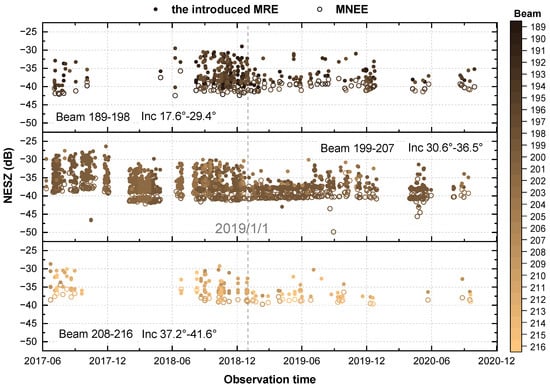
Figure 3. The NESZ evaluation results of the GaoFen-3’s QPSI mode from June 2017 to September 2020. The three stacked plots represent the noise estimation in different imaging beams, distinguished in different colors. Inc means the nominal incident angle. The solid scatters are the introduced MRE measurements, and the circle scatters denote the lower estimation by MNEE [3].

Figure 3 shows 28 beams of QPSI that have been divided into three groups, which were used to analyze the NESZ level. The products mainly appear in the beams numbered 199 to 207. In this group, the NESZ slightly yearly decreased during the first three years until January 2019. In 2017, the early stage of the system operation, the NESZ may have exceeded −30 dB for certain middle beams. Since February 2018, the system NESZ values have been almost lower than −30 dB. For the months after 1 January 2019, the NESZ is even below −35 dB. We believe that the system quality indicator NESZ has been improved since the inflight operation. The measurements using the introduced MRE present the total results of all orbits of the same day. In addition, the MNEE preserves the minimum level among all the calculations in one day and derives the fitting prediction. Consequently, as shown in Figure 3, the acquired MNEE circle scatters always represent the lower estimation of the NESZ, which is shown as a reference. Throughout the four-year mid-range MNEE results, the estimated NESZ varies mainly between −42.5 and −37.5 dB, which demonstrates that the GaoFen-3 system is able to control the noise at a low level with the improved target-identification capability and can obtain a high SNR for QPSI products.

3.2. Radiometric Resolution

Highly stochastic Amazon rainforests are ideal natural targets for evaluating GaoFen-3 radiometric resolution. Eight leading imaging modes were assessed with the collected Amazon datasets. We selected the co-pol intensity images (i.e., HH\VV) in the experiment and utilized the empirical thresholds to segment the forest samples. Then, Equation (8) was used based on the measured ENL to deduce the radiometric resolution level for the single-pol, dual-pol and quad-pol datasets. In the same manner, we categorized the datasets of the same beam code in one day by orbit using the SegmentID field in the header files. The refined orbit strip results are shown in Figure 4. The light gray horizontal line in the figure is the specification level, 3 dB, for products of a nominal spatial resolution of approximately 1 to 10 m, while the satellite is in orbit [8]. All the measurements range between 2.4 and 2.9 dB, which is better than the system design. A smaller radiometric resolution level is generally known to allow better accuracy in the quantitative interpretation of SAR images. Thus, in theory, efforts could be made to minimize Equation (8) from the system inputs for radiometric resolution optimization, such as imposing $SNR=0 \mathrm{dB}$ or setting the maximum bandwidth that is permitted for the system [25]. However, the potential conflict with other SAR parameters that is caused by a rising bandwidth will be troublesome. Therefore, to further improve the image radiometric resolution, the ENL can be increased in the preprocessing stage.

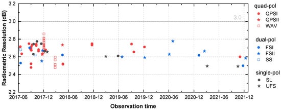
Figure 4. GaoFen-3’s radiometric resolution assessment based on single-pol, dual-pol, and quad-pol strip datasets, which were acquired from the Amazon rainforest from June 2017 to December 2021. The results are summarized for all imaging modes from the data with the same orbit and beam code on the same day. Red represents the results of three different quad-pol modes, QPSI, QPSII, and WAV; blue represents the results of the FSI, FSII, and SS modes; and black represents the results of the SL and UFS modes.

3.3. Spatial Resolution

A few datasets in the Inner Mongolia calibration site are mainly acquired in the summer season, and the representative TCR impulse responses are shown in Figure 5.

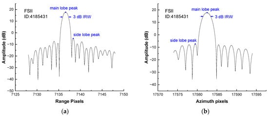
Figure 5. Sample TCR impulse responses in the (a) range and (b) azimuth directions.

On the basis of the average 3 dB IRW of all the TCRs imaged in the Inner Mongolia calibration site, according to Equation (2), the spatial resolution analysis in the range and azimuth directions from June 2017 to September 2021 is shown in Figure 6. The measured spatial resolution in the azimuth direction in Figure 6b, theoretically governed by the length of the radar antenna, is stable over five years, with an overall average of 1.02, 2.96, 4.83, 9.55, 7.38, and 7.65 m for SL, UFS, FSI, FSII, SS and QPSI modes, respectively; these are almost consistent with the nominal level in the corresponding header files. The estimated spatial resolution in the range direction in Figure 6a is generally higher than that in the azimuth direction. Furthermore, it varies differently even for products with the same imaging mode, which is proportional to the transmitting bandwidth [20]. For example, the SL mode holds an invariable bandwidth in the range look of 240 MHz, allowing a nominal range resolution of 0.625 m, if the IRW broadening factor is ignored. As shown in Figure 6a, the average estimation of SS products in the calibration site is approximately 0.65 m, which is in good agreement with the expected level. For other imaging modes, the range bandwidth in the header files is found to occasionally change. Thus, the estimation presents an unstable result in contrast to that found in the azimuth direction.

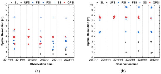
Figure 6. GaoFen-3’s spatial resolution evaluation on single-pol, dual-pol, and quad-pol datasets for the Inner Mongolia calibration site from June 2017 to October 2021. (a) Spatial resolution results in the range direction; and (b) results in the azimuth direction.

3.4. PSLR and ISLR

The assessment of PSLR in the range and azimuth directions was based on Equation (3); the results are shown in Figure 7. The design specification of PSLR is −20 dB, as presented by the horizontal light gray line in the figure. Most measurements satisfy the design specification level and may be as low as −26 dB. Exceeding values can also be observed for a few products, which may be explained by the strong backscattering from the surrounding artificial objects. Moreover, the TCR impulse response profiles of the products are occasionally found to be non-standard. It is unclear whether TCRs are properly deployed in the Inner Mongolia prairie. The CRs are generally meant to be installed facing against the direction of the radar line of sight, as well as placed in the ground without dense vegetation or other artificial constructions.

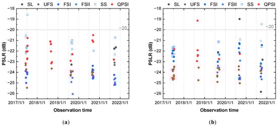
Figure 7. GaoFen-3’s PSLR evaluation on single-pol, dual-pol, and quad-pol datasets for the Inner Mongolia calibration site from June 2017 to October 2021. (a) and (b) are the results in the range and azimuth directions, respectively.

The one-dimensional ISLR estimation with CR impulse responses in the range and azimuth directions is shown in Figure 8, according to Equation (4). The horizontal light gray line represents the design specification level of the ISLR, which was noted to be −13 dB. The result for the azimuth direction shown in Figure 8b, which is important for the motion effects on system quality, meets the system design. Exceeding these specifications still occurs in range direction estimation. High integrated side lobe energy was attributed not only to the nature of the side lobes, but also to the distributions of scattering around the deployed CRs within the scene [21]. In addition to the installation of various CRs, the antenna patterns should be checked to determine whether they have been compensated for in the imaging process [29]. For the imaging modes, such as UFS, FSI, FSII, SS, and QPSI, the fields ElevationPatternCorrection and AmuthPatternCorrection in the header file are sometimes displayed as 0. That is, the antenna patterns have not been appropriately corrected even for the published products. The fields relevant to the radiometric and polarimetric characteristics must be carefully verified, and whether the image quality can be relied upon should be justified.

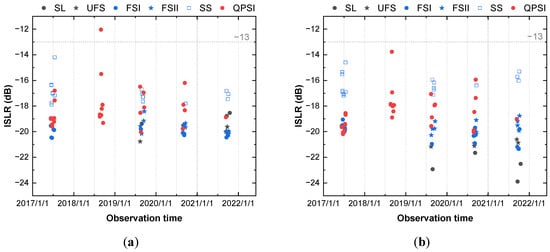
Figure 8. GaoFen-3’s ISLR estimation in Inner Mongolia with CR datasets acquired from June 2017 to October 2021. (a) Results in the range direction; and (b) the azimuth results.

3.5. Relative Radiation Correction Accuracy

The relative radiation correction accuracy calculation aims to evaluate the radar radiometric stability based on the returned CR scattering of the same type and size. The measured RCS of CRs is obtained via the integral method in Equation (5). First, a square target window (8 $\times$ 8) centered on the CR peak is opened. The integrated power in the cross area, excluding the energy $E_{clt}$ in the four background clutter quadrants, is the normalized RCS $E_{CR}$ in the resolution cell. Then, the CR RCS ${\sigma }_{CR}$ is computed by multiplying the integrated point target energy with the area A of the resolution cell. All the measured RCS values of the CR targets in a single image can determine the relative radiation correction accuracy via Equation (6). The results of these different imaging modes are shown in Figure 9. The estimation results were generated with the CRs in scenes, such that the analysis actually refers to the radiation accuracy in 0.1–0.2 s of flight time, according to the location of CRs in the azimuth direction and the acquisition time of a single image. For GaoFen-3’s standard products, the relative radiation correction accuracy is designed to be no more than 1.0 dB. The calculation in Figure 9 is approximately 0.01–0.51 dB, which is better than the design specification, thereby demonstrating that GaoFen-3 provides a good radiation performance with high stability and accuracy during five years of operation.

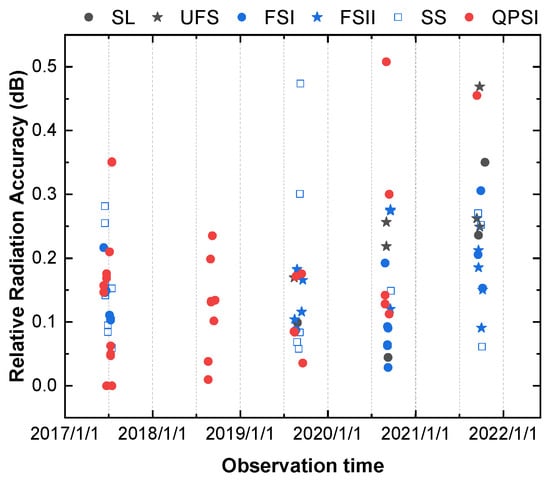
Figure 9. GaoFen-3’s relative radiation correction accuracy evaluation using the Inner Mongolia datasets from June 2017 to October 2021. The estimation of each scatter is based on the CR responses in a single image.

4. Polarimetric Validation

4.1. Crosstalk

For the GaoFen-3 products, the crosstalk should not exceed −35 dB. The modified Quegan method mentioned in Equation (25) was used for estimating the distortions in the quad-pol datasets. First, the common scattering features were combined to extract distributed forest samples with empirical thresholds, that is, $R_{HHVV}\le 0.4$, $R_{HVVH}\ge 0.8$ and $ENL\ge 0.3$. Then, with the calibration model and using TR and RTAS constraints, the $\alpha$-preserving criterion ${\mathsf{{\rm P}}}_{\left|\alpha \right|}$ helped the search for the optimal crosstalk solution. In the experiment, the search can be finished in the fifth recalibration. The estimated $\widehat{u}, \widehat{v}, \widehat{w}, \widehat{z}$, together with the channel imbalance $\widehat{k}$ and $\widehat{\alpha }$, were substituted into the calibration model, regarding the true scattering coefficients as ${\left[\begin{array}{cccc}1& 0& 0& 1\end{array}\right]}^T$, for the purpose of simulated observations in order to calculate channel ratios. The amplitude ratio of HV and VV was analyzed to assess the measured crosstalk level, as shown in Figure 10. It should be noted that the amplitude of the HV/VV channel ratio calculation follows the example of TCR measurements, and may be smaller than the crosstalk levels. The evaluation results for the quad-pol imagery in Figure 10 do not exceed the −40 dB specification. In addition, the estimation of QPSII and WAV both satisfy the design specification, as observed from the collected datasets. Overall, the GaoFen-3 crosstalk of the quad-pol imaging modes has performed well over the last five years.

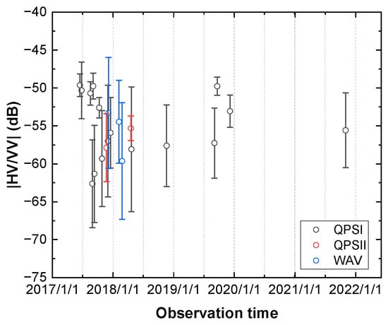
Figure 10. GaoFen-3’s crosstalk evaluation based on the modified Quegan method with Amazon forests datasets of QPSI, QPSII, and WAV modes from June 2017 to November 2021. Here, we present the mean and standard deviation (std) measurements of the HV/VV channel ratio in amplitude with the calculated polarimetric distortions from the forest samples.

4.2. Cross-Pol Channel Imbalance

GaoFen-3’s cross-pol channel imbalance is designed with no more than a 0.5 dB amplitude error and 10° phase error. The estimated cross-pol channel imbalance is based on the modified Quegan method using forest samples, after determining the crosstalk solutions. Additionally, the cross-pol channel ratio results are used to represent the cross-pol channel imbalance amplitude and phase, as shown in Figure 11. The estimation results in terms of both amplitude and phase are stable and vary in a small range for the three imaging modes. In particular, the cross-pol channel imbalance amplitude of the QPSII mode exceeds the 0.5 dB specification, while the phase error out of the specification, approximately 0.62°, mainly occurs in the WAV mode. The errors in the cross-pol channel imbalance during the five years are not severe and can be well-calibrated, as long as there are sufficient vegetation samples in the scene.

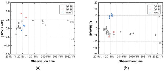
Figure 11. GaoFen-3’s cross-pol channel imbalance assessment using the modified Quegan method in the Amazon rainforest from June 2017 to November 2021. The channel ratios between HV and VH were calculated. (a) The cross-pol channel imbalance amplitude; and (b) the cross-pol channel imbalance phase.

4.3. Co-Pol Channel Imbalance

The GaoFen-3 co-pol channel imbalance is also designed with an amplitude level that is better than 0.5 dB and a phase that does not exceed 10°. In the rainforest datasets, after estimating and calibrating the crosstalk and cross-pol channel imbalance distortions, we can obtain the remaining co-pol channel imbalance k via the co-pol channel ratio in Equations (29) and (30). In Figure 12, we present the amplitude and phase results on the basis of the HH and VV channel ratios. The co-pol channel ratios were derived from the simulated observations for which we substitute all polarimetric distortions into the calibration model. Thus, the results shown in Figure 12 are mainly due to the cross-pol and co-pol channel imbalance estimates. Compared with the cross-pol channel imbalance in Figure 11, there are non-negligible errors in the quad-pol imaging mode. Moreover, the k amplitude and phase calculations appear to change in a slightly large range. The amplitude error out of the specification, approximately −0.28 dB, can be noted for the QPSII mode from 2017 to 2020; the phase error is significant in the WAV mode and can reach −14.38°. The evaluation of GaoFen-3’s polarimetric quality in the Amazon rainforest reminds us that greater attention should be directed to channel imbalance errors, especially for the less common imaging modes.

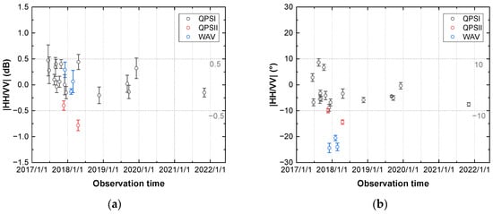
Figure 12. GaoFen-3’s co-pol channel imbalance evaluation with the Amazon rainforest datasets from June 2017 to November 2021, based on HH and VV channel ratios. (a) The co-pol channel imbalance amplitude; and (b) the co-pol channel imbalance phase.

4.4. Polarimetric Calibration

The modified Quegan method was used for estimating the distortions in the standard products of the QPSI, QPSII, and WAV modes during the last five years. The results shown in Figure 11 and Figure 12 indicate that there are potential channel imbalance errors in some of the imagery. We categorized the estimated distortions by orbit and refined the orbit distortions as strip estimators to calibrate the Amazon rainforest products of three imaging modes, as well as calculating the average residual distortion error in each orbit, as shown in Table 2. The errors are presented with the amplitude and phase results of ratios between the co-pol and cross-pol terms and refer to the residual co-pol channel imbalance, and cross-pol channel imbalance in different orbits. Here, we also expect a channel imbalance amplitude of no more than 0.5 dB and phase within ±10°. As shown in Table 2, all the residuals satisfy the specification level. The estimated co-pol channel imbalance amplitude was between −0.02 and 0.02 dB, and the phase ranged from −0.51° to 0.51°. The residual cross-pol channel imbalance error was even lower at −0.02 dB and −0.001° on average, as dense vegetation accurately helped to calibrate the strip imagery. The validation experiment demonstrated that the modified Quegan method works effectively for polarimetric calibration with strip measurements.

Table 2. The residual distortion error validation of the QPSI, QPSII and WAV modes with the Amazon rainforest datasets, after calibration with the strip estimators. The last four columns represent the residual amplitude and phase of the co-pol channel imbalance, and the cross-pol channel imbalance.

Time	Mode	Beam	Orbit ID	|HH/VV| (dB)	∠HH/VV (°)	|HV/VH| (dB)	∠HV/VH (°)
2017/6/16	QPSI	190	4476	−0.0022	0.0811	0.0066	−0.0024
2017/6/26	QPSI	208	4622	0.0030	−0.1630	0.0007	0.0036
2017/8/18	QPSI	189	5383	−0.0076	0.5058	−0.0030	0.0172
2017/8/30	QPSI	195	5564	−0.0009	−0.5091	−0.0035	0.0016
2017/9/4	QPSI	194	5628	−0.0071	−0.1438	−0.0036	0.0037
2017/9/11	QPSI	199	5739	−0.0021	−0.3230	−0.0068	−0.0065
2017/10/10	QPSI	189	6148	−0.0017	−0.2635	−0.0056	0.0243
2017/10/27	QPSI	194	6392	−0.0007	−0.4809	−0.0058	0.0044
2017/12/2	QPSI	203	6918	−0.0091	−0.1249	−0.0101	−0.0275
2017/12/17	QPSI	200	7127	−0.0072	−0.0070	−0.0098	0.0008
2018/4/22	QPSI	213	8944	−0.0019	−0.0987	0.0101	−0.0002
2018/11/20	QPSI	198	12,006	−0.0267	−0.0369	−0.0095	0.0020
2019/9/4	QPSI	193	16,158	−0.0208	0.0333	−0.0098	0.0079
2019/9/21	QPSI	207	16,396	−0.0176	0.0062	−0.0165	0.0182
2019/12/7	QPSI	191	17,506	0.0231	0.0058	−0.0059	0.0092
2021/11/2	QPSI	203	27,540	−0.0020	0.0402	−0.0123	0.0085
2017/11/23	QPSII	225	6782	−0.0008	−0.0523	−0.1409	−0.0604
2018/4/19	QPSII	219	8900	−0.0053	0.0707	−0.1106	−0.0550
2017/12/5	WAV	200	6955	−0.0246	0.1807	0.0082	0.0128
2018/2/6	WAV	211	7863	−0.0001	0.0233	−0.0132	0.0063
2018/2/25	WAV	205	8136	0.0007	−0.3791	−0.0123	0.0077

5. Discussion

For GaoFen-3’s operation in orbit from June 2017 to December 2021, nine radiometric and polarimetric characteristics were evaluated based on CRAS with the datasets that were acquired in the Chinese mainland, Amazon rainforest, and the Inner Mongolia calibration site. These are summarized in Table 3.

Table 3. Summary of GaoFen-3’s radiometric and polarimetric characteristics in orbit from June 2017 to December 2021. The measurements exceeding the design specification are marked in red. The last column, colored in gray, presents the performance of the Canadian Radarsat-2 Fine Quad (FQ) mode.

	SL/UFS	FSI/FSII/SS	QPSI/QPSII/WAV	Radarsat-2 FQ Performance
NESZ	-	-	<−30 dB	<−32 dB
Radiometric resolution	2.80 dB	2.80 dB	2.90 dB	-
Spatial resolution	1.02/2.96 m	4.83/9.55/7.38 m	7.65 m	7.60 m
PSLR	−21.5 dB	−21 dB	−20 dB	-
ISLR	−18 dB	−14 dB	−14 dB	-
Relative radiation accuracy	0.1–0.2 s, <0.47 dB	<0.47 dB	<0.51 dB	15 s, <1 dB; mission life, <3 dB
Crosstalk	-	-	<−40/−46/−41 dB	<−40 dB
Cross-pol channel imbalance	-	-	0.17/0.75/0.07 dB −2.99/−4.49/9.82°	±0.30 dB ±3°
Co-pol channel imbalance	-	-	0.14/−0.59/0.07 dB −3.09/−12.19/−22.95°	±0.30 dB ±3°

Compared with the early test result in Ref. [8], the NESZ measured using LBOs in the long strip in this study has been improved by approximately 10 dB for the QPSI mode. Furthermore, there is little difference in contrast to the performance of the Radarsat-2 Fine Quad mode. The radiometric resolution was measured based on the Amazon rainforest and is below 2.9 dB, which is superior to the 3 dB test result for the imagery of the 1~10 m resolution in Ref. [8]. The spatial resolution calculated using the CR responses presented in Table 3 refers to that in the azimuth direction. The spatial resolution of the QPSI mode was almost consistent with the performance of Radarsat-2. The PSLR here was slightly higher than the tested −22 dB in Ref. [8], and the averaged ISLR differed in different imaging modes. As stated in the last section, the antenna pattern in the range and azimuth directions was not always compensated for while checking the fields in the product header files. In addition, the measured RCS of the CR targets may deviate from its theoretical value, and thus occasionally affect the traditional absolute radiation accuracy. The relative radiation accuracy measured using CRs in a single image is good, whether compared with the test result in Ref. [8] or with the requirement of Radarsat-2, which demonstrates that the imaging in the azimuth direction is stable. With regard to the GaoFen-3’s system polarimetric quality, the crosstalk was estimated below −40 dB for the quad-pol products after October 2017, which coincides with the system specification, but out-of-specification occurred for some modes in the channel imbalance amplitude and phase, as highlighted in red in Table 3. The polarimetric calibration via the proposed modified Quegan method with strip estimators can remove the channel imbalance errors and improve the image quality, as shown by the validation results in Table 2. The polarimetric analysis in rainforests was convenient and efficient, as the distortions can be illustrated and calibrated accordingly. However, for the usual scenes without dense vegetation, solving all of the distortions accurately requires more effort.

6. Conclusions

This study derived the CRAS framework to evaluate GaoFen-3’s radiometric and polarimetric quality over its five-year operation period. Among the evaluation parameters, the radiometric performance can better satisfy the original system’s design specification. NESZ was estimated to be less than −30 dB from February 2018 and even lower than −35 dB for the months after January 2019. The calculation of the radiometric resolution ranges between 2.4 and 2.9 dB for the eight leading modes over five years, and they are better than the system design of 3 dB for products with a spatial resolution of 1–10 m. The azimuthal spatial resolution of the products acquired in the calibration site among all the modes was measured with a stable result from June 2017 to October 2021, and the results were very close to the nominal specification in the header files. The relative radiation accuracy based on the CRs in the azimuth direction of a single product can reach the requirement of Radarsat-2. Furthermore, the polarimetric quality requires additional enhancement. The crosstalk estimates using the modified Quegan method over five years were almost below −40 dB, consistent with the system design. However, distortion bias occurred in the amplitude and phase of the channel imbalance for the QPSII and WAV modes since November 2017, which may make a difference in further precise applications, such as quantitative parameter estimation. In the future, we will continuously focus on measuring and calibrating the channel imbalance distortion to a global extent, and promote the polarimetric assessment of dual-pol products, thoroughly evaluating the system level for users’ reference.

References

- Lee, J.-S.; Pottier, E. Polarimetric Radar Imaging: From Basics to Applications; CRC Press: Boca Raton, FL, USA, 2009. [Google Scholar]
- Zyl, J.V.; Kim, Y. Synthetic Aperture Radar Polarimetry; Wiley: Hoboken, NJ, USA, 2011. [Google Scholar]
- Shi, L.; Yang, L.; Zhao, L.; Li, P.; Yang, J.; Zhang, L. NESZ Estimation and Calibration for Gaofen-3 Polarimetric Products by the Minimum Noise Envelope Estimator. IEEE Trans. Geosci. Remote Sens. 2020, 59, 7517–7534. [Google Scholar] [CrossRef]
- Chang, Y.; Li, P.; Yang, J.; Zhao, J.; Zhao, L.; Shi, L. Polarimetric Calibration and Quality Assessment of the GF-3 Satellite Images. Sensors 2018, 18, 403. [Google Scholar] [CrossRef] [PubMed]
- Shi, L.; Li, P.; Yang, J.; Zhang, L.; Ding, X.; Zhao, L. Polarimetric Channel Misregistration Evaluation for the GaoFen-3 QPSI Mode. IEEE Geosci. Remote Sens. Lett. 2019, 16, 544–548. [Google Scholar] [CrossRef]
- Li, X.-M.; Zhang, T.; Huang, B.; Jia, T. Capabilities of Chinese Gaofen-3 Synthetic Aperture Radar in Selected Topics for Coastal and Ocean Observations. Remote Sens. 2018, 10, 1929. [Google Scholar] [CrossRef]
- Zhang, T.; Yang, Y.; Shokr, M.; Mi, C.; Li, X.-M.; Cheng, X.; Hui, F. Deep Learning Based Sea Ice Classification with Gaofen-3 Fully Polarimetric SAR Data. Remote Sens. 2021, 13, 1452. [Google Scholar] [CrossRef]
- Zhang, Q. System Design and Key Technologies of the GF-3 Satellite. Acta Geod. Cartogr. Sin. 2017, 46, 269–277. [Google Scholar]
- Liang, W.; Jia, Z.; Qiu, X.; Hong, J.; Zhang, Q.; Lei, B.; Zhang, F.; Deng, Z.; Wang, A. Polarimetric Calibration of the GaoFen-3 Mission Using Active Radar Calibrators and the Applicable Conditions of System Model for Radar Polarimeters. Remote Sens. 2019, 11, 176. [Google Scholar] [CrossRef]
- Chen, Q.; Li, Z.; Zhang, P.; Tao, H.; Zeng, J. A Preliminary Evaluation of the GaoFen-3 SAR Radiation Characteristics in Land Surface and Compared With Radarsat-2 and Sentinel-1A. IEEE Geosci. Remote Sens. Lett. 2018, 15, 1040–1044. [Google Scholar] [CrossRef]
- Shi, L.; Li, P.; Yang, J.; Sun, H.; Zhao, L.; Zhang, L. Polarimetric calibration for the distributed Gaofen-3 product by an improved unitary zero helix framework. ISPRS J. Photogramm. Remote Sens. 2020, 160, 229–243. [Google Scholar] [CrossRef]
- Shangguan, S.; Qiu, X.; Fu, K.; Lei, B.; Hong, W. GF-3 Polarimetric Data Quality Assessment Based on Automatic Extraction of Distributed Targets. IEEE J. Sel. Top. Appl. Earth Obs. Remote Sens. 2020, 13, 4282–4294. [Google Scholar] [CrossRef]
- Sun, G.; Li, Z.; Huang, L.; Chen, Q.; Zhang, P. Quality analysis and improvement of polarimetric synthetic aperture radar (SAR) images from the GaoFen-3 satellite using the Amazon rainforest as an example. Int. J. Remote Sens. 2021, 42, 2131–2154. [Google Scholar] [CrossRef]
- Shi, L.; Li, P.; Yang, J.; Zhang, L.; Ding, X.; Zhao, L. Co-polarization channel imbalance phase estimation by corner-reflector-like targets. ISPRS J. Photogramm. Remote Sens. 2019, 147, 255–266. [Google Scholar] [CrossRef]
- Quegan, S. A unified algorithm for phase and cross-talk calibration of polarimetric data-theory and observations. IEEE Trans. Geosci. Remote Sens. 1994, 32, 89–99. [Google Scholar] [CrossRef]
- Yang, L.; Shi, L.; Yang, J.; Li, P.; Zhao, L.; Zhao, J. PolSAR additive noise estimation based on shadow regions. Int. J. Remote Sens. 2021, 42, 259–273. [Google Scholar] [CrossRef]
- Ainsworth, T.L.; Ferro-Famil, L.; Jong-Sen, L. Orientation angle preserving a posteriori polarimetric SAR calibration. IEEE Trans. Geosci. Remote Sens. 2006, 44, 994–1003. [Google Scholar] [CrossRef]
- Xing, S.; Dai, D.; Liu, J.; Wang, X. Comment on “Orientation Angle Preserving A Posteriori Polarimetric SAR Calibration”. IEEE Trans. Geosci. Remote Sens. 2012, 50, 2417–2419. [Google Scholar] [CrossRef]
- Freeman, A. SAR calibration: An overview. IEEE Trans. Geosci. Remote Sens. 1992, 30, 1107–1121. [Google Scholar] [CrossRef]
- Cumming, I.G.; Wong, F.H. Digital processing of synthetic aperture radar data. Artech House 2005, 1, 108–110. [Google Scholar]
- Carrara, W.G.; Goodman, R.S.; Majewski, R.M. Spotlight Synthetic Aperture Radar: Signal Processing Algorithms; Artech House: Boston, MA, USA; London, UK, 1995. [Google Scholar]
- Garthwaite, M.; Nancarrow, S.; Hislop, A.; Thankappan, M.; Dawson, J.; Lawrie, S. Design of radar corner reflectors for the Australian Geophysical Observing System. Geosci. Aust. 2015, 3, 490. [Google Scholar]
- Luscombe, A.P. RADARSAT-2 SAR image quality and calibration operations. Can. J. Remote Sens. 2004, 30, 345–354. [Google Scholar] [CrossRef]
- Hajnsek, I.; Papathanassiou, K.P.; Cloude, S.R. Removal of Additive Noise in Polarimetric Eigenvalue Processing. In Proceedings of the IEEE International Geoscience and Remote Sensing Symposium, Sydney, Australia, 9–13 July 2001; Volume 6, pp. 2778–2780. [Google Scholar]
- Marquez-Martinez, J.; Mittermayer, J.; Rodriguez-Cassola, M. Radiometric Resolution Optimization for Future SAR Systems. In Proceedings of the IGARSS 2004. 2004 IEEE International Geoscience and Remote Sensing Symposium, Anchorage, AK, USA, 20–24 September 2004; Volume 1733, pp. 1738–1741. [Google Scholar]
- Luscombe, A. Image Quality and Calibration of RADARSAT-2. In Proceedings of the 2009 IEEE International Geoscience and Remote Sensing Symposium, Cape Town, South Africa, 12–17 July 2009; pp. II-757–II-760. [Google Scholar]
- Tan, H.; Hong, J. Calibration of Compact Polarimetric SAR Images Using Distributed Targets and One Corner Reflector. IEEE Trans. Geosci. Remote Sens. 2016, 54, 4433–4444. [Google Scholar] [CrossRef]
- Olivier, P.; Vidal-Madjar, D. Empirical estimation of the ERS-1 SAR radiometric resolution. Int. J. Remote Sens. 1994, 15, 1109–1114. [Google Scholar] [CrossRef]
- Shimada, M.; Isoguchi, O.; Tadono, T.; Isono, K. PALSAR Radiometric and Geometric Calibration. IEEE Trans. Geosci. Remote Sens. 2009, 47, 3915–3932. [Google Scholar] [CrossRef]
- Arii, M.; Zyl, J.J.V.; Kim, Y. Adaptive Model-Based Decomposition of Polarimetric SAR Covariance Matrices. IEEE Trans. Geosci. Remote Sens. 2011, 49, 1104–1113. [Google Scholar] [CrossRef]
- Zyl, J.J.V.; Arii, M.; Kim, Y. Model-Based Decomposition of Polarimetric SAR Covariance Matrices Constrained for Nonnegative Eigenvalues. IEEE Trans. Geosci. Remote Sens. 2011, 49, 3452–3459. [Google Scholar]
- Lee, J.S.; Grunes, M.R.; Kwok, R. Classification of multi-look polarimetric SAR imagery based on complex Wishart distribution. Int. J. Remote Sens. 1994, 15, 2299–2311. [Google Scholar] [CrossRef]
Disclaimer/Publisher’s Note: The statements, opinions and data contained in all publications are solely those of the individual author(s) and contributor(s) and not of MDPI and/or the editor(s). MDPI and/or the editor(s) disclaim responsibility for any injury to people or property resulting from any ideas, methods, instructions or products referred to in the content. |
© 2023 by the authors. Licensee MDPI, Basel, Switzerland. This article is an open access article distributed under the terms and conditions of the Creative Commons Attribution (CC BY) license (https://creativecommons.org/licenses/by/4.0/).