
Radiometric and Polarimetric Quality Validation of Gaofen-3 over a Five-Year Operation Period

 , , ,
, , ,  and
and 
Abstract
1. Introduction
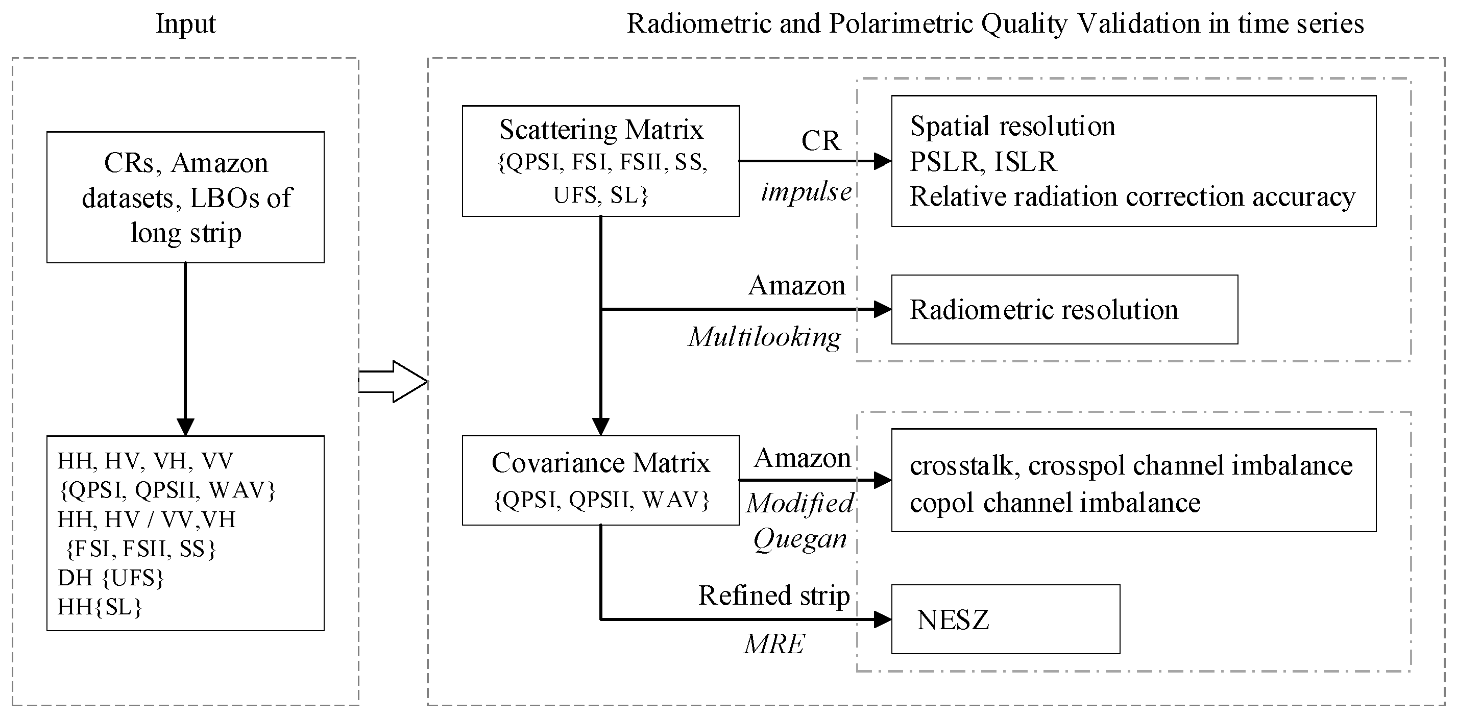
2. The Derived CRAS
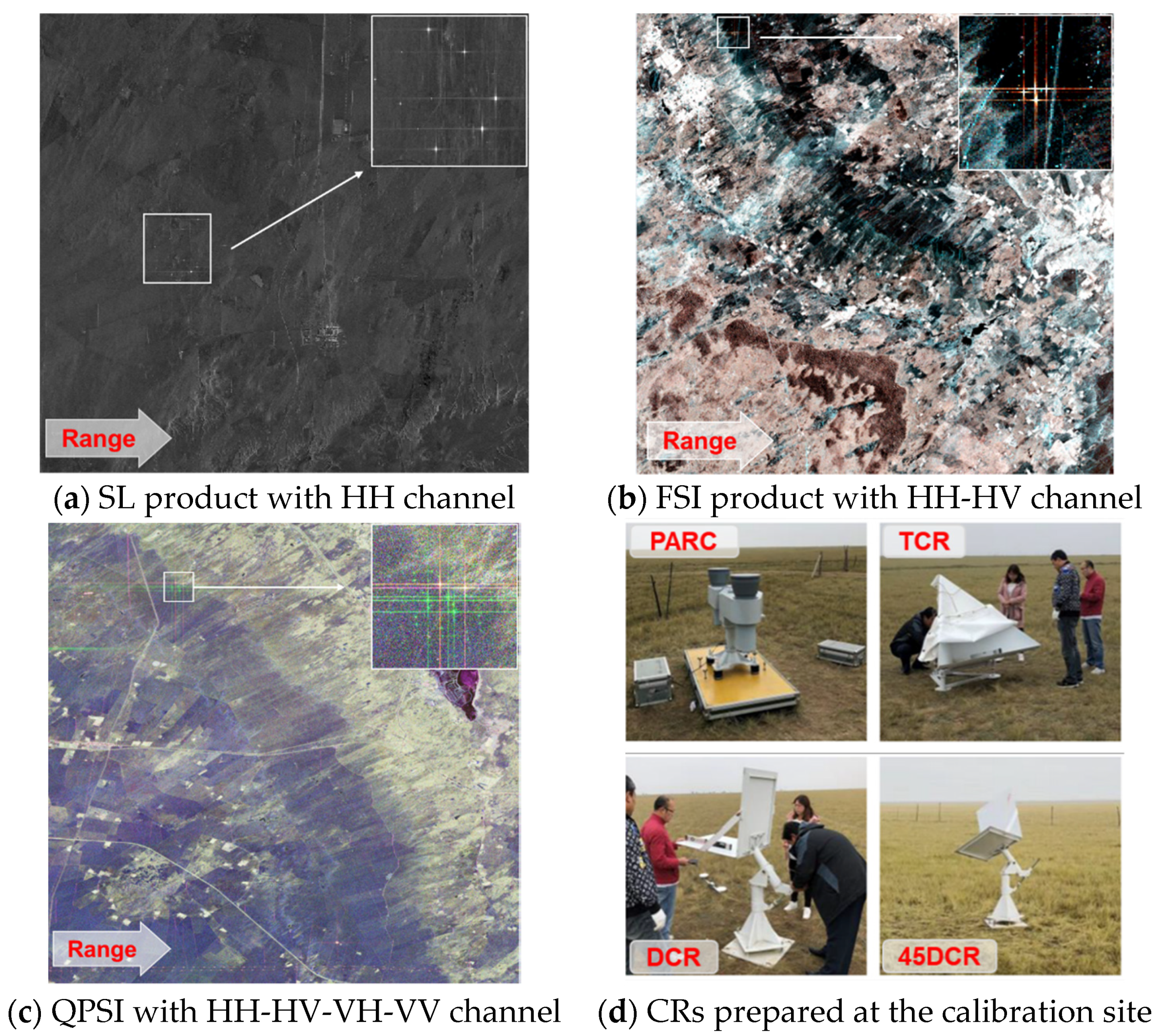
2.1. CR Response for System Quality
2.2. Natural Observation for System Evaluation
2.3. Modified Quegan Method for Polarimetric Distortions
3. Image Quality Evaluation
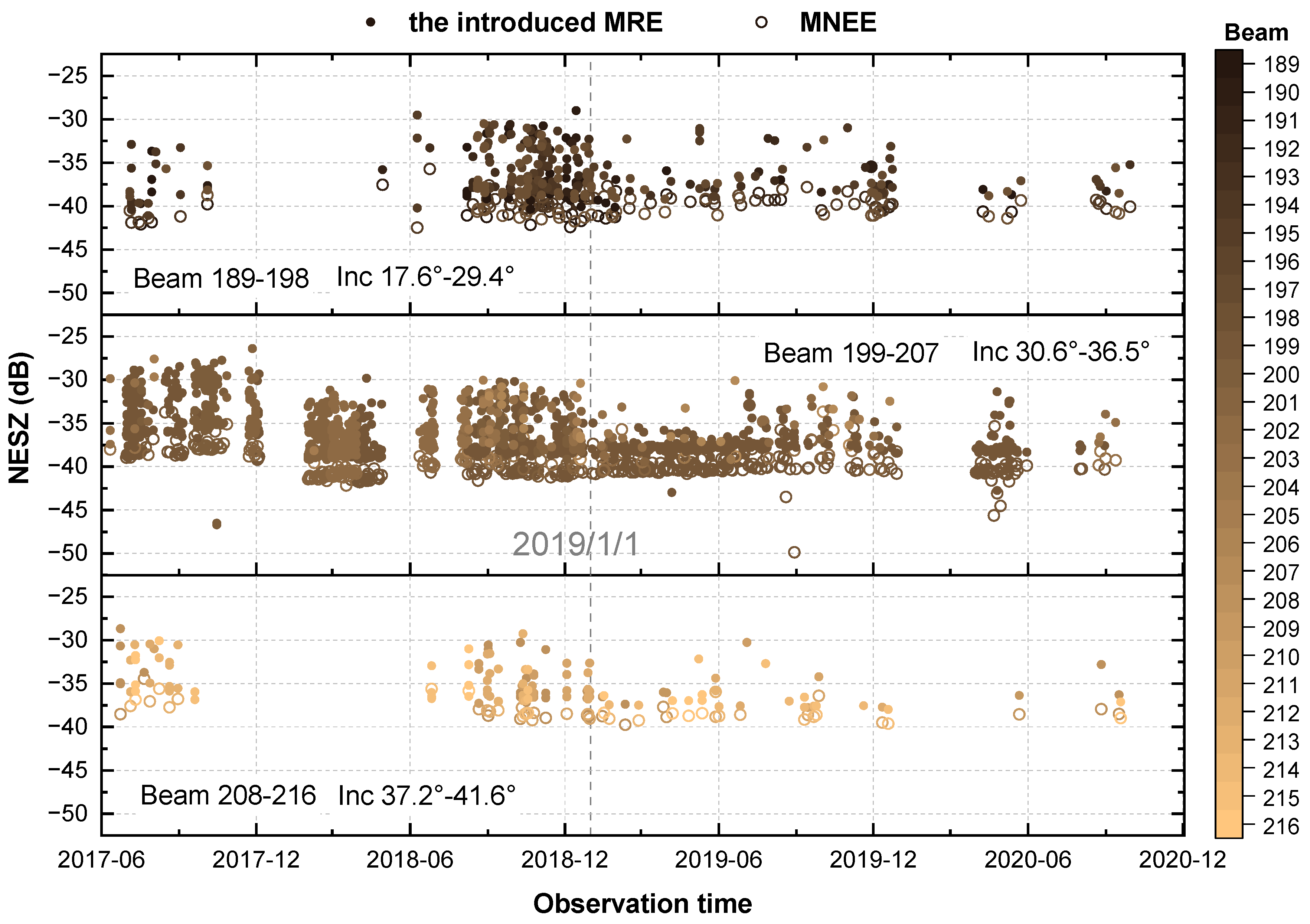
3.1. NESZ
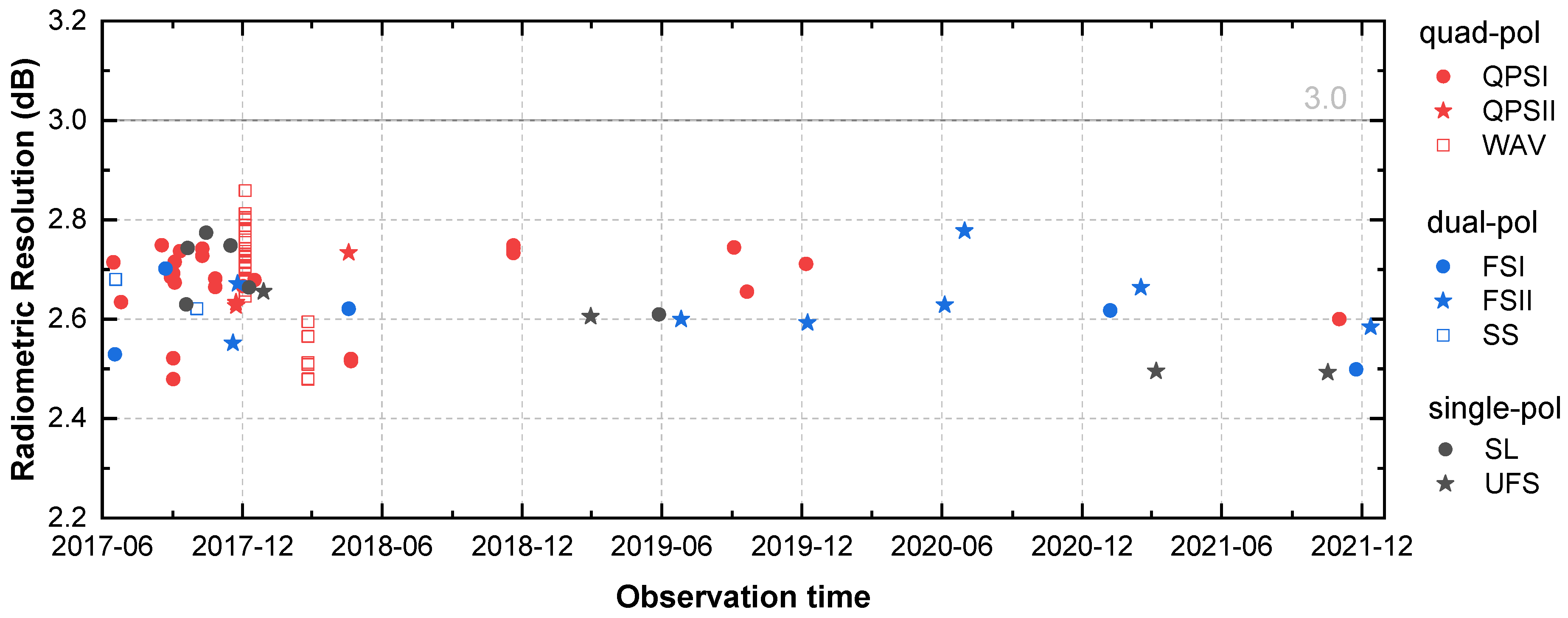
3.2. Radiometric Resolution
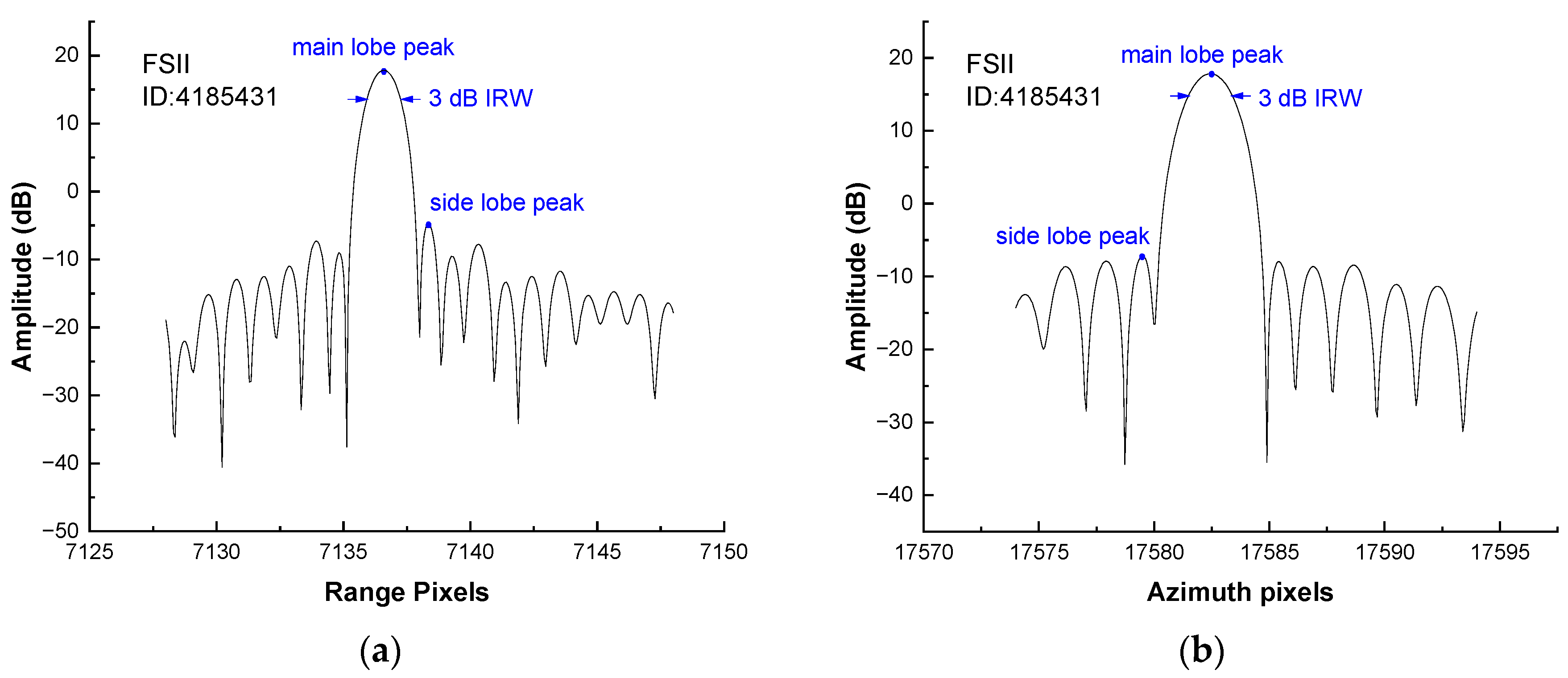
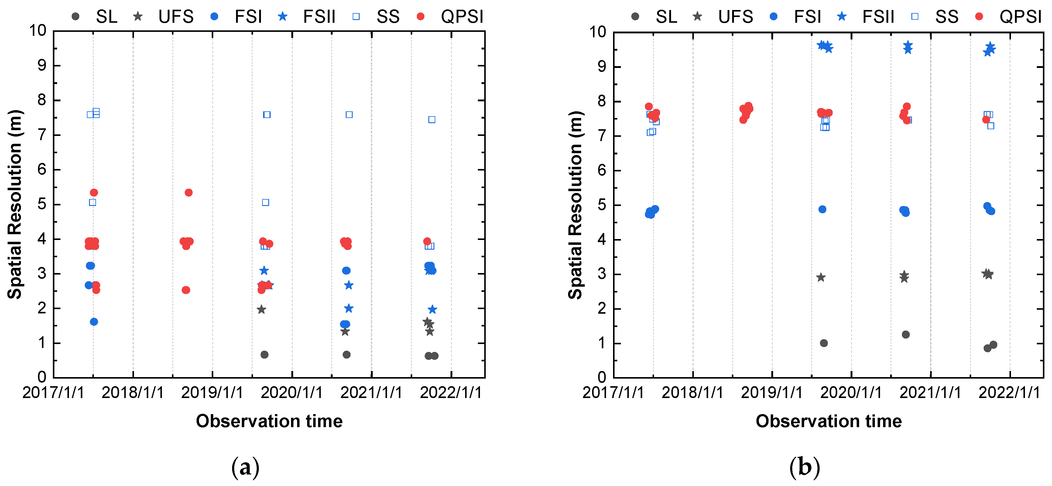
3.3. Spatial Resolution
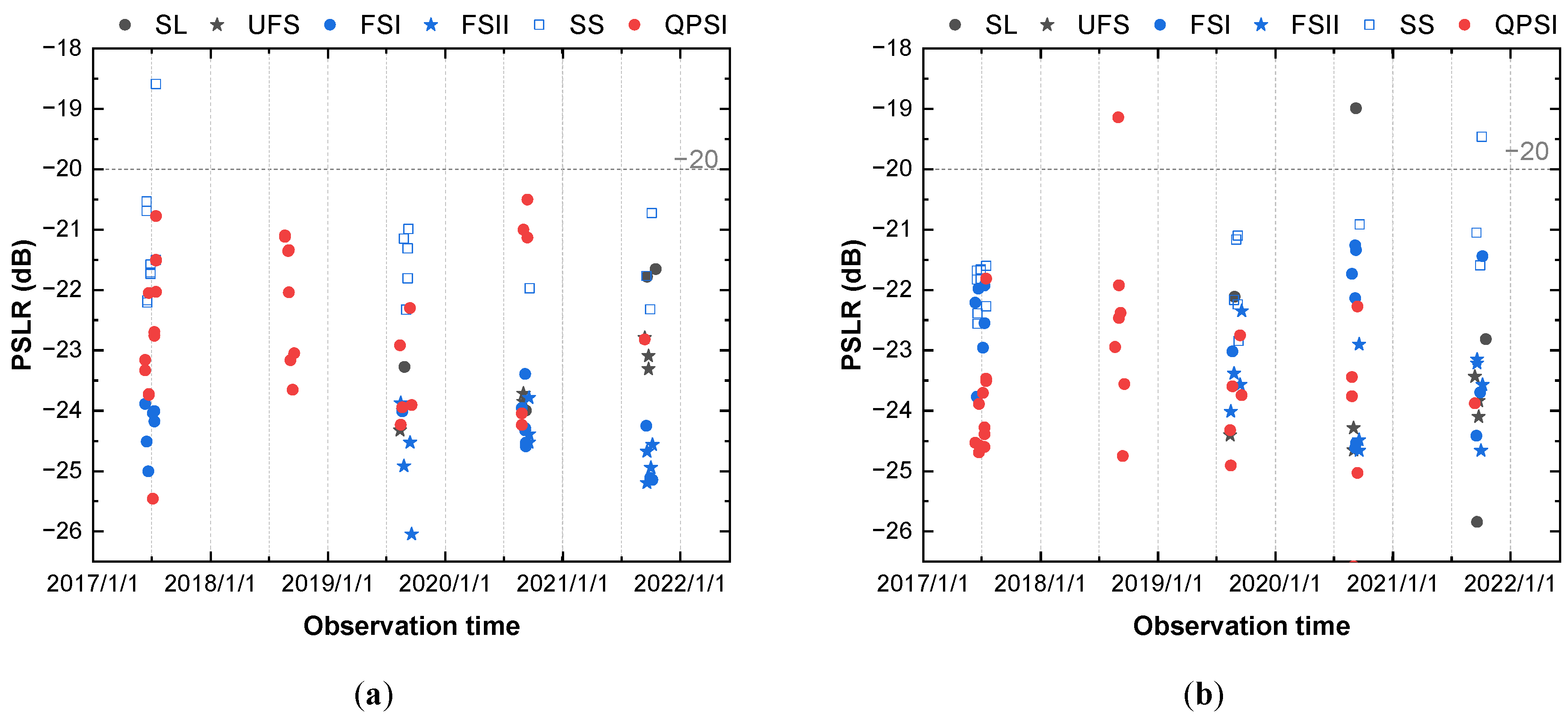
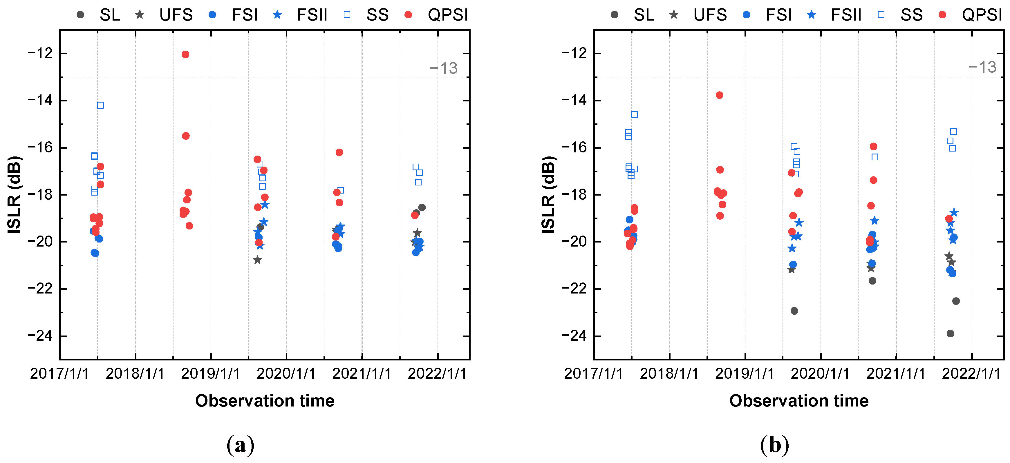
3.4. PSLR and ISLR
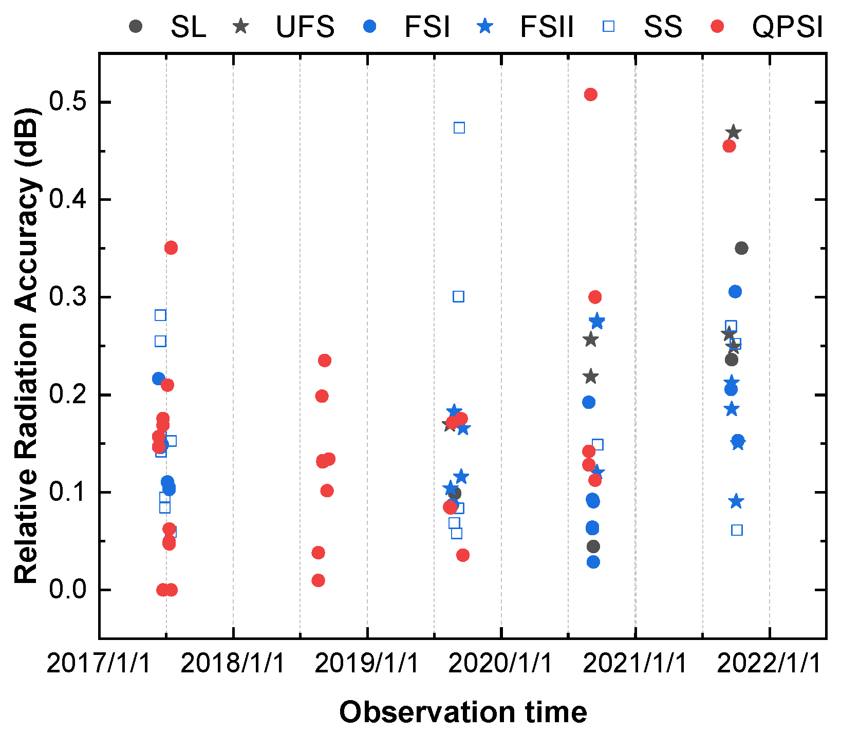
3.5. Relative Radiation Correction Accuracy
4. Polarimetric Validation
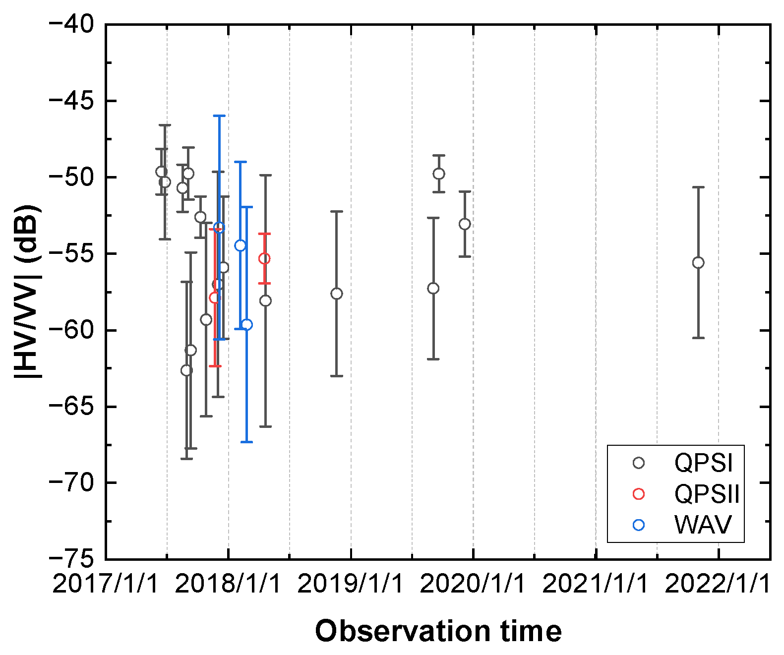
4.1. Crosstalk
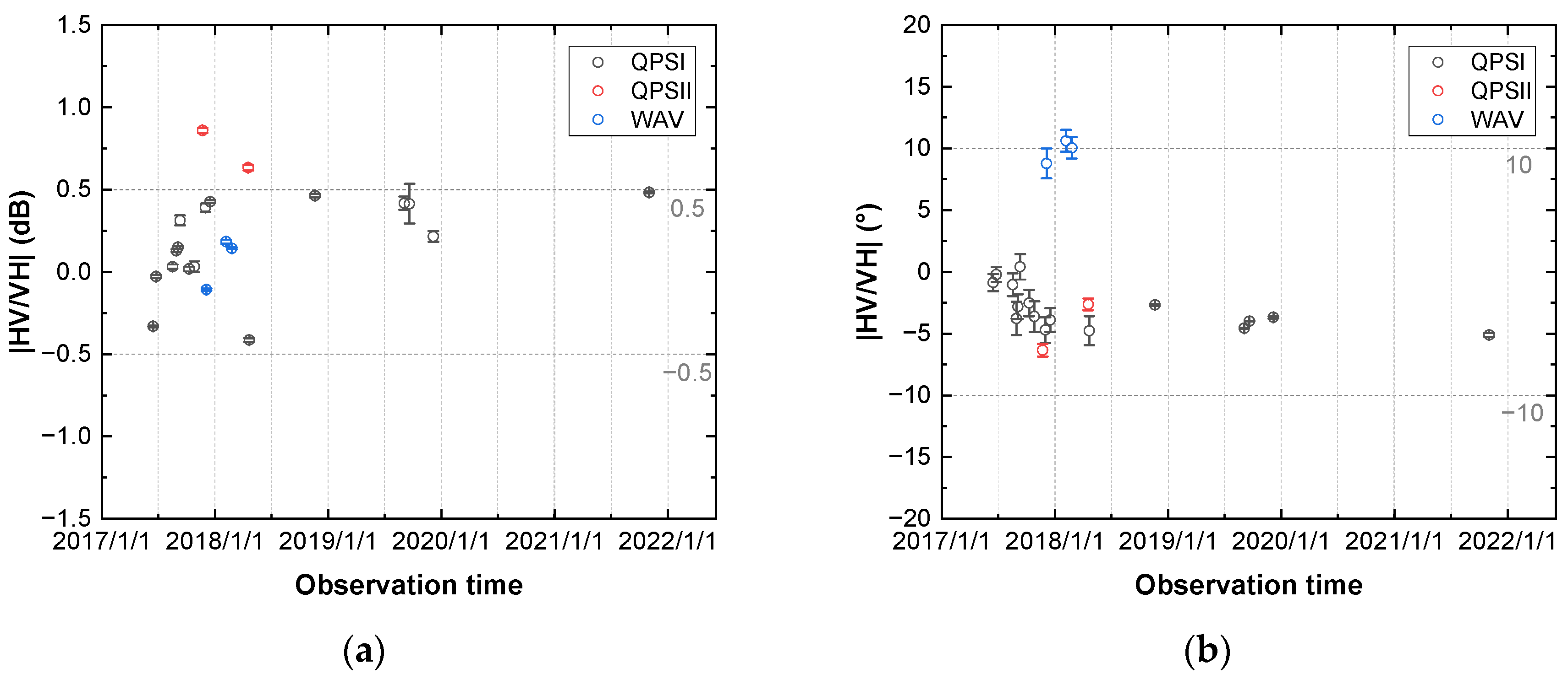
4.2. Cross-Pol Channel Imbalance
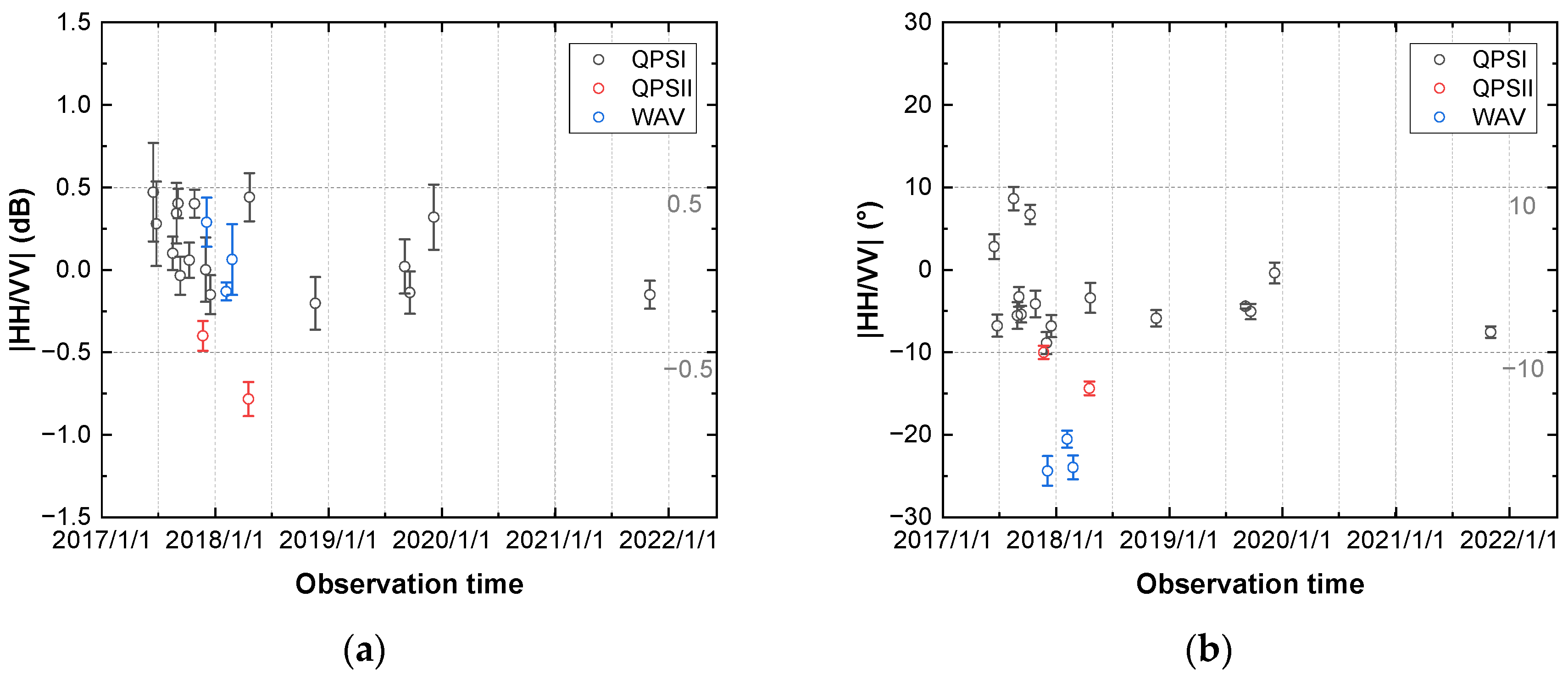
4.3. Co-Pol Channel Imbalance
4.4. Polarimetric Calibration
5. Discussion
6. Conclusions
Author Contributions
Funding
Data Availability Statement
Conflicts of Interest
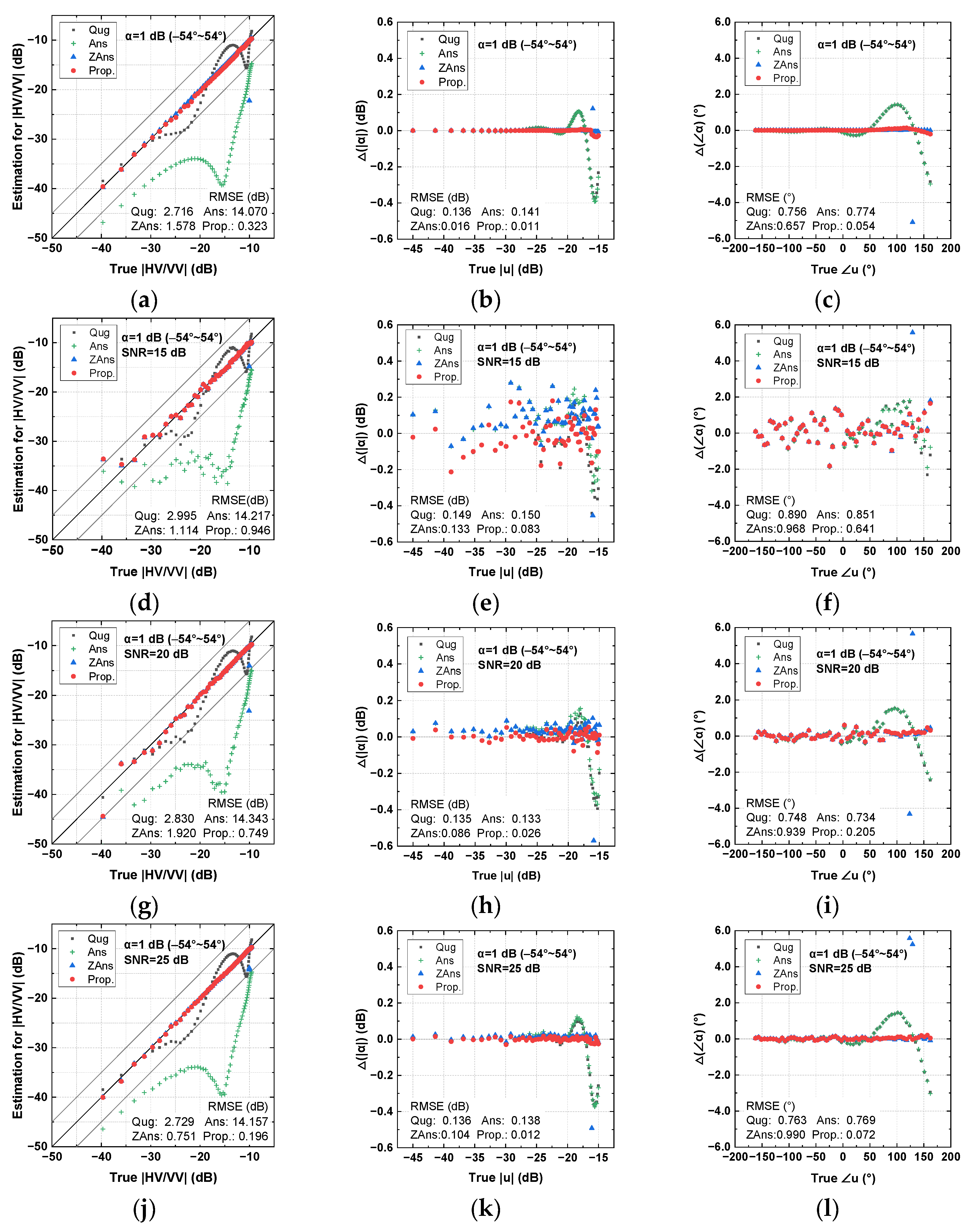
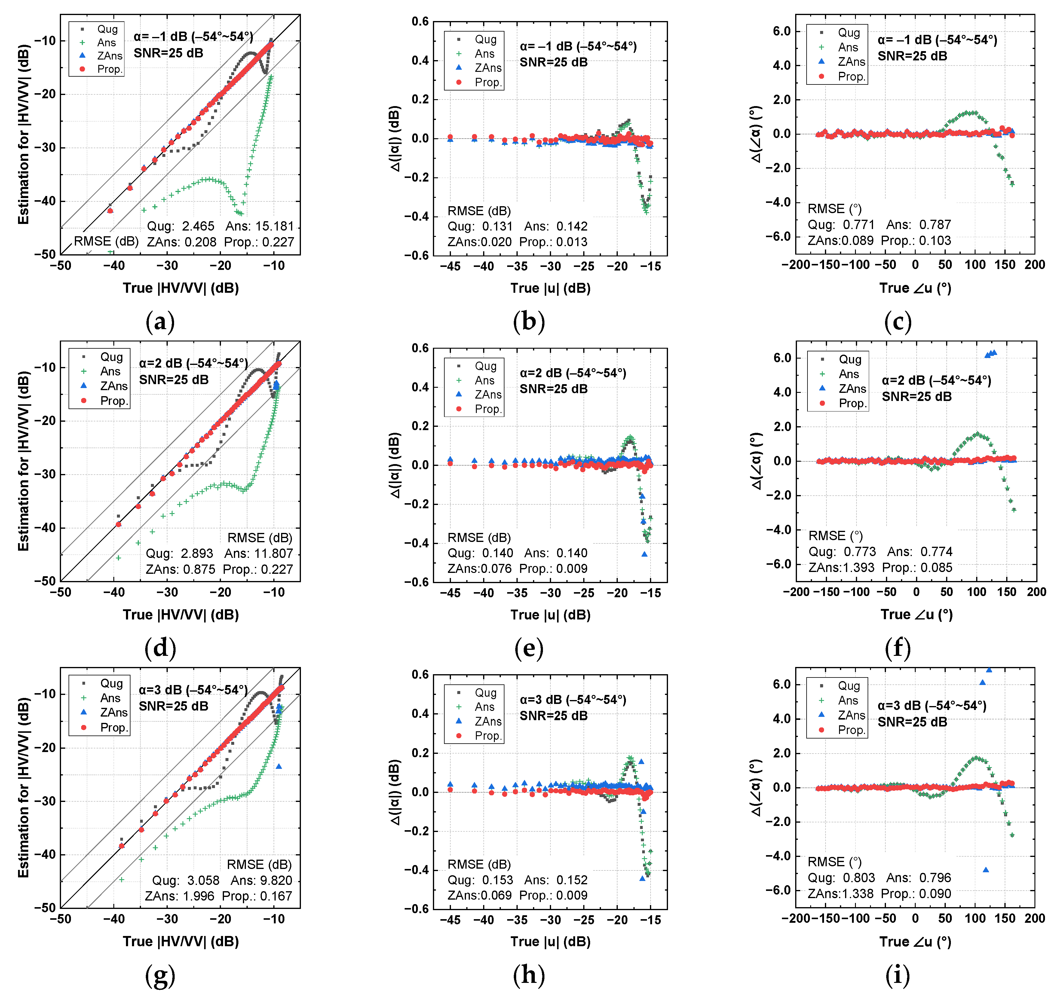
Appendix A. Quantitative analysis of the modified Quegan Method

| u | v | w | z | k | ||
|---|---|---|---|---|---|---|
| Amplitude (dB) | (−45, −15) | |u| | |u| | |u| | −1; 1; 2; 3 | 0 |
| Phase (rad) | (−0.9, 0.9) | ∠u + 0.08 | ∠u + 0.14 | ∠u + 0.17 | (−0.3, 0.3) | 0 |


References
- Lee, J.-S.; Pottier, E. Polarimetric Radar Imaging: From Basics to Applications; CRC Press: Boca Raton, FL, USA, 2009. [Google Scholar]
- Zyl, J.V.; Kim, Y. Synthetic Aperture Radar Polarimetry; Wiley: Hoboken, NJ, USA, 2011. [Google Scholar]
- Shi, L.; Yang, L.; Zhao, L.; Li, P.; Yang, J.; Zhang, L. NESZ Estimation and Calibration for Gaofen-3 Polarimetric Products by the Minimum Noise Envelope Estimator. IEEE Trans. Geosci. Remote Sens. 2020, 59, 7517–7534. [Google Scholar] [CrossRef]
- Chang, Y.; Li, P.; Yang, J.; Zhao, J.; Zhao, L.; Shi, L. Polarimetric Calibration and Quality Assessment of the GF-3 Satellite Images. Sensors 2018, 18, 403. [Google Scholar] [CrossRef] [PubMed]
- Shi, L.; Li, P.; Yang, J.; Zhang, L.; Ding, X.; Zhao, L. Polarimetric Channel Misregistration Evaluation for the GaoFen-3 QPSI Mode. IEEE Geosci. Remote Sens. Lett. 2019, 16, 544–548. [Google Scholar] [CrossRef]
- Li, X.-M.; Zhang, T.; Huang, B.; Jia, T. Capabilities of Chinese Gaofen-3 Synthetic Aperture Radar in Selected Topics for Coastal and Ocean Observations. Remote Sens. 2018, 10, 1929. [Google Scholar] [CrossRef]
- Zhang, T.; Yang, Y.; Shokr, M.; Mi, C.; Li, X.-M.; Cheng, X.; Hui, F. Deep Learning Based Sea Ice Classification with Gaofen-3 Fully Polarimetric SAR Data. Remote Sens. 2021, 13, 1452. [Google Scholar] [CrossRef]
- Zhang, Q. System Design and Key Technologies of the GF-3 Satellite. Acta Geod. Cartogr. Sin. 2017, 46, 269–277. [Google Scholar]
- Liang, W.; Jia, Z.; Qiu, X.; Hong, J.; Zhang, Q.; Lei, B.; Zhang, F.; Deng, Z.; Wang, A. Polarimetric Calibration of the GaoFen-3 Mission Using Active Radar Calibrators and the Applicable Conditions of System Model for Radar Polarimeters. Remote Sens. 2019, 11, 176. [Google Scholar] [CrossRef]
- Chen, Q.; Li, Z.; Zhang, P.; Tao, H.; Zeng, J. A Preliminary Evaluation of the GaoFen-3 SAR Radiation Characteristics in Land Surface and Compared With Radarsat-2 and Sentinel-1A. IEEE Geosci. Remote Sens. Lett. 2018, 15, 1040–1044. [Google Scholar] [CrossRef]
- Shi, L.; Li, P.; Yang, J.; Sun, H.; Zhao, L.; Zhang, L. Polarimetric calibration for the distributed Gaofen-3 product by an improved unitary zero helix framework. ISPRS J. Photogramm. Remote Sens. 2020, 160, 229–243. [Google Scholar] [CrossRef]
- Shangguan, S.; Qiu, X.; Fu, K.; Lei, B.; Hong, W. GF-3 Polarimetric Data Quality Assessment Based on Automatic Extraction of Distributed Targets. IEEE J. Sel. Top. Appl. Earth Obs. Remote Sens. 2020, 13, 4282–4294. [Google Scholar] [CrossRef]
- Sun, G.; Li, Z.; Huang, L.; Chen, Q.; Zhang, P. Quality analysis and improvement of polarimetric synthetic aperture radar (SAR) images from the GaoFen-3 satellite using the Amazon rainforest as an example. Int. J. Remote Sens. 2021, 42, 2131–2154. [Google Scholar] [CrossRef]
- Shi, L.; Li, P.; Yang, J.; Zhang, L.; Ding, X.; Zhao, L. Co-polarization channel imbalance phase estimation by corner-reflector-like targets. ISPRS J. Photogramm. Remote Sens. 2019, 147, 255–266. [Google Scholar] [CrossRef]
- Quegan, S. A unified algorithm for phase and cross-talk calibration of polarimetric data-theory and observations. IEEE Trans. Geosci. Remote Sens. 1994, 32, 89–99. [Google Scholar] [CrossRef]
- Yang, L.; Shi, L.; Yang, J.; Li, P.; Zhao, L.; Zhao, J. PolSAR additive noise estimation based on shadow regions. Int. J. Remote Sens. 2021, 42, 259–273. [Google Scholar] [CrossRef]
- Ainsworth, T.L.; Ferro-Famil, L.; Jong-Sen, L. Orientation angle preserving a posteriori polarimetric SAR calibration. IEEE Trans. Geosci. Remote Sens. 2006, 44, 994–1003. [Google Scholar] [CrossRef]
- Xing, S.; Dai, D.; Liu, J.; Wang, X. Comment on “Orientation Angle Preserving A Posteriori Polarimetric SAR Calibration”. IEEE Trans. Geosci. Remote Sens. 2012, 50, 2417–2419. [Google Scholar] [CrossRef]
- Freeman, A. SAR calibration: An overview. IEEE Trans. Geosci. Remote Sens. 1992, 30, 1107–1121. [Google Scholar] [CrossRef]
- Cumming, I.G.; Wong, F.H. Digital processing of synthetic aperture radar data. Artech House 2005, 1, 108–110. [Google Scholar]
- Carrara, W.G.; Goodman, R.S.; Majewski, R.M. Spotlight Synthetic Aperture Radar: Signal Processing Algorithms; Artech House: Boston, MA, USA; London, UK, 1995. [Google Scholar]
- Garthwaite, M.; Nancarrow, S.; Hislop, A.; Thankappan, M.; Dawson, J.; Lawrie, S. Design of radar corner reflectors for the Australian Geophysical Observing System. Geosci. Aust. 2015, 3, 490. [Google Scholar]
- Luscombe, A.P. RADARSAT-2 SAR image quality and calibration operations. Can. J. Remote Sens. 2004, 30, 345–354. [Google Scholar] [CrossRef]
- Hajnsek, I.; Papathanassiou, K.P.; Cloude, S.R. Removal of Additive Noise in Polarimetric Eigenvalue Processing. In Proceedings of the IEEE International Geoscience and Remote Sensing Symposium, Sydney, Australia, 9–13 July 2001; Volume 6, pp. 2778–2780. [Google Scholar]
- Marquez-Martinez, J.; Mittermayer, J.; Rodriguez-Cassola, M. Radiometric Resolution Optimization for Future SAR Systems. In Proceedings of the IGARSS 2004. 2004 IEEE International Geoscience and Remote Sensing Symposium, Anchorage, AK, USA, 20–24 September 2004; Volume 1733, pp. 1738–1741. [Google Scholar]
- Luscombe, A. Image Quality and Calibration of RADARSAT-2. In Proceedings of the 2009 IEEE International Geoscience and Remote Sensing Symposium, Cape Town, South Africa, 12–17 July 2009; pp. II-757–II-760. [Google Scholar]
- Tan, H.; Hong, J. Calibration of Compact Polarimetric SAR Images Using Distributed Targets and One Corner Reflector. IEEE Trans. Geosci. Remote Sens. 2016, 54, 4433–4444. [Google Scholar] [CrossRef]
- Olivier, P.; Vidal-Madjar, D. Empirical estimation of the ERS-1 SAR radiometric resolution. Int. J. Remote Sens. 1994, 15, 1109–1114. [Google Scholar] [CrossRef]
- Shimada, M.; Isoguchi, O.; Tadono, T.; Isono, K. PALSAR Radiometric and Geometric Calibration. IEEE Trans. Geosci. Remote Sens. 2009, 47, 3915–3932. [Google Scholar] [CrossRef]
- Arii, M.; Zyl, J.J.V.; Kim, Y. Adaptive Model-Based Decomposition of Polarimetric SAR Covariance Matrices. IEEE Trans. Geosci. Remote Sens. 2011, 49, 1104–1113. [Google Scholar] [CrossRef]
- Zyl, J.J.V.; Arii, M.; Kim, Y. Model-Based Decomposition of Polarimetric SAR Covariance Matrices Constrained for Nonnegative Eigenvalues. IEEE Trans. Geosci. Remote Sens. 2011, 49, 3452–3459. [Google Scholar]
- Lee, J.S.; Grunes, M.R.; Kwok, R. Classification of multi-look polarimetric SAR imagery based on complex Wishart distribution. Int. J. Remote Sens. 1994, 15, 2299–2311. [Google Scholar] [CrossRef]


| Observations | Location | Time | Imaging Mode | Number of Images |
|---|---|---|---|---|
| Calibration site | Inner Mongolia, China | 2017.6–2021.9 | SL/UFS FSI/FSII/SS QPSI | 4/6 16/11/21 32 |
| Rainforest | Amazon, Brazil | 2017.6–2021.12 | SL/UFS FSI/FSII/SS QPSI/QPSII/WAV | 7/114 83/58/19 525/41/41 |
| Long strips | Chinese Mainland | 2017.6–2020.9 | QPSI | 39,929 |
| Time | Mode | Beam | Orbit ID | |HH/VV| (dB) | ∠HH/VV (°) | |HV/VH| (dB) | ∠HV/VH (°) |
|---|---|---|---|---|---|---|---|
| 2017/6/16 | QPSI | 190 | 4476 | −0.0022 | 0.0811 | 0.0066 | −0.0024 |
| 2017/6/26 | QPSI | 208 | 4622 | 0.0030 | −0.1630 | 0.0007 | 0.0036 |
| 2017/8/18 | QPSI | 189 | 5383 | −0.0076 | 0.5058 | −0.0030 | 0.0172 |
| 2017/8/30 | QPSI | 195 | 5564 | −0.0009 | −0.5091 | −0.0035 | 0.0016 |
| 2017/9/4 | QPSI | 194 | 5628 | −0.0071 | −0.1438 | −0.0036 | 0.0037 |
| 2017/9/11 | QPSI | 199 | 5739 | −0.0021 | −0.3230 | −0.0068 | −0.0065 |
| 2017/10/10 | QPSI | 189 | 6148 | −0.0017 | −0.2635 | −0.0056 | 0.0243 |
| 2017/10/27 | QPSI | 194 | 6392 | −0.0007 | −0.4809 | −0.0058 | 0.0044 |
| 2017/12/2 | QPSI | 203 | 6918 | −0.0091 | −0.1249 | −0.0101 | −0.0275 |
| 2017/12/17 | QPSI | 200 | 7127 | −0.0072 | −0.0070 | −0.0098 | 0.0008 |
| 2018/4/22 | QPSI | 213 | 8944 | −0.0019 | −0.0987 | 0.0101 | −0.0002 |
| 2018/11/20 | QPSI | 198 | 12,006 | −0.0267 | −0.0369 | −0.0095 | 0.0020 |
| 2019/9/4 | QPSI | 193 | 16,158 | −0.0208 | 0.0333 | −0.0098 | 0.0079 |
| 2019/9/21 | QPSI | 207 | 16,396 | −0.0176 | 0.0062 | −0.0165 | 0.0182 |
| 2019/12/7 | QPSI | 191 | 17,506 | 0.0231 | 0.0058 | −0.0059 | 0.0092 |
| 2021/11/2 | QPSI | 203 | 27,540 | −0.0020 | 0.0402 | −0.0123 | 0.0085 |
| 2017/11/23 | QPSII | 225 | 6782 | −0.0008 | −0.0523 | −0.1409 | −0.0604 |
| 2018/4/19 | QPSII | 219 | 8900 | −0.0053 | 0.0707 | −0.1106 | −0.0550 |
| 2017/12/5 | WAV | 200 | 6955 | −0.0246 | 0.1807 | 0.0082 | 0.0128 |
| 2018/2/6 | WAV | 211 | 7863 | −0.0001 | 0.0233 | −0.0132 | 0.0063 |
| 2018/2/25 | WAV | 205 | 8136 | 0.0007 | −0.3791 | −0.0123 | 0.0077 |
| SL/UFS | FSI/FSII/SS | QPSI/QPSII/WAV | Radarsat-2 FQ Performance | |
|---|---|---|---|---|
| NESZ | - | - | <−30 dB | <−32 dB |
| Radiometric resolution | 2.80 dB | 2.80 dB | 2.90 dB | - |
| Spatial resolution | 1.02/2.96 m | 4.83/9.55/7.38 m | 7.65 m | 7.60 m |
| PSLR | −21.5 dB | −21 dB | −20 dB | - |
| ISLR | −18 dB | −14 dB | −14 dB | - |
| Relative radiation accuracy | 0.1–0.2 s, <0.47 dB | <0.47 dB | <0.51 dB | 15 s, <1 dB; mission life, <3 dB |
| Crosstalk | - | - | <−40/−46/−41 dB | <−40 dB |
| Cross-pol channel imbalance | - | - | 0.17/0.75/0.07 dB −2.99/−4.49/9.82° | ±0.30 dB ±3° |
| Co-pol channel imbalance | - | - | 0.14/−0.59/0.07 dB −3.09/−12.19/−22.95° | ±0.30 dB ±3° |
Disclaimer/Publisher’s Note: The statements, opinions and data contained in all publications are solely those of the individual author(s) and contributor(s) and not of MDPI and/or the editor(s). MDPI and/or the editor(s) disclaim responsibility for any injury to people or property resulting from any ideas, methods, instructions or products referred to in the content. |
© 2023 by the authors. Licensee MDPI, Basel, Switzerland. This article is an open access article distributed under the terms and conditions of the Creative Commons Attribution (CC BY) license (https://creativecommons.org/licenses/by/4.0/).
Share and Cite
Yang, L.; Shi, L.; Sun, W.; Yang, J.; Li, P.; Li, D.; Liu, S.; Zhao, L. Radiometric and Polarimetric Quality Validation of Gaofen-3 over a Five-Year Operation Period. Remote Sens. 2023, 15, 1605. https://doi.org/10.3390/rs15061605
Yang L, Shi L, Sun W, Yang J, Li P, Li D, Liu S, Zhao L. Radiometric and Polarimetric Quality Validation of Gaofen-3 over a Five-Year Operation Period. Remote Sensing. 2023; 15(6):1605. https://doi.org/10.3390/rs15061605
Chicago/Turabian StyleYang, Le, Lei Shi, Weidong Sun, Jie Yang, Pingxiang Li, Deren Li, Shanwei Liu, and Lingli Zhao. 2023. "Radiometric and Polarimetric Quality Validation of Gaofen-3 over a Five-Year Operation Period" Remote Sensing 15, no. 6: 1605. https://doi.org/10.3390/rs15061605
APA StyleYang, L., Shi, L., Sun, W., Yang, J., Li, P., Li, D., Liu, S., & Zhao, L. (2023). Radiometric and Polarimetric Quality Validation of Gaofen-3 over a Five-Year Operation Period. Remote Sensing, 15(6), 1605. https://doi.org/10.3390/rs15061605