

Applying UAV-Based Remote Sensing Observation Products in High Arctic Catchments in SW Spitsbergen


Abstract
1. Introduction
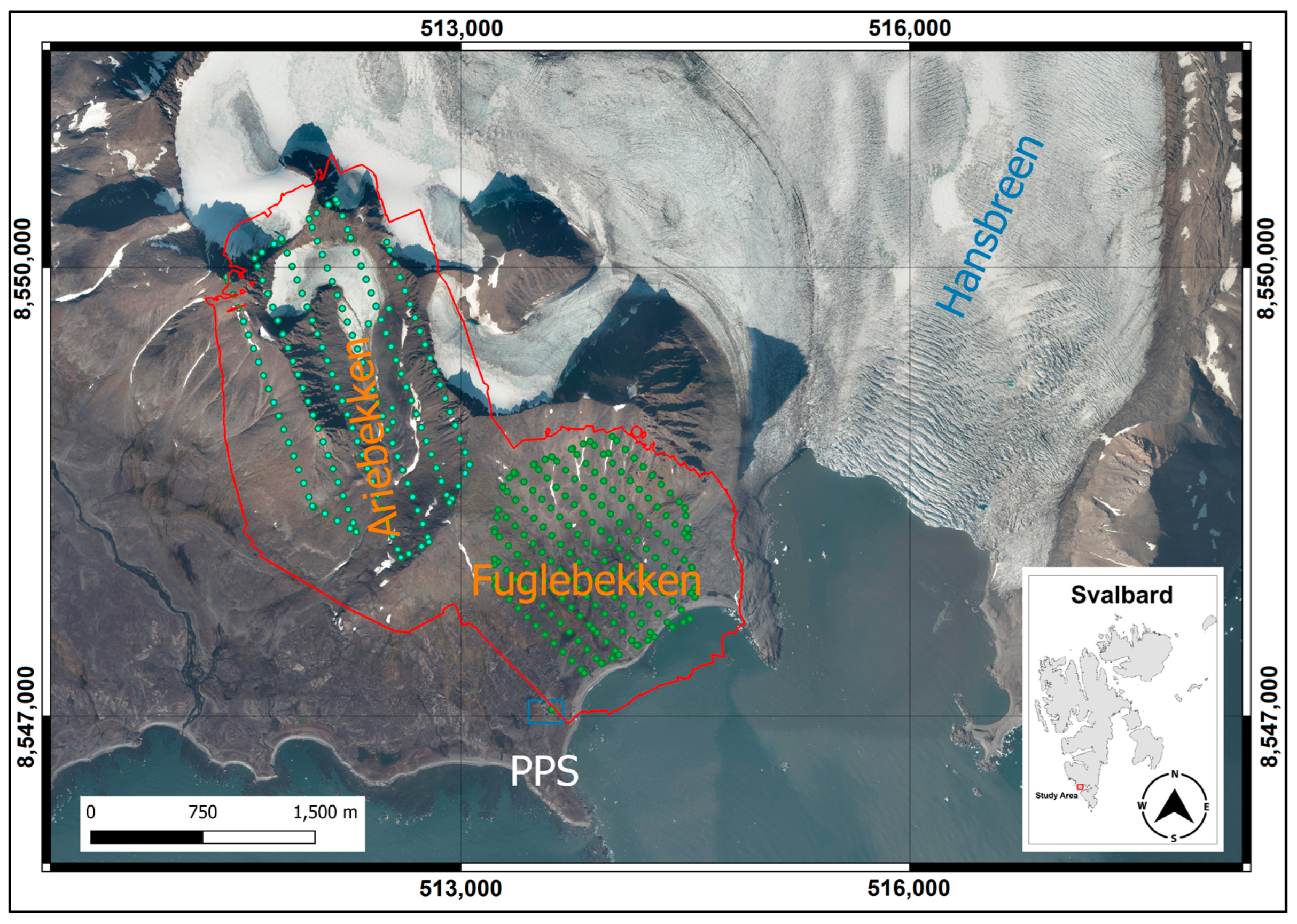
2. Study Area
3. Materials and Methods
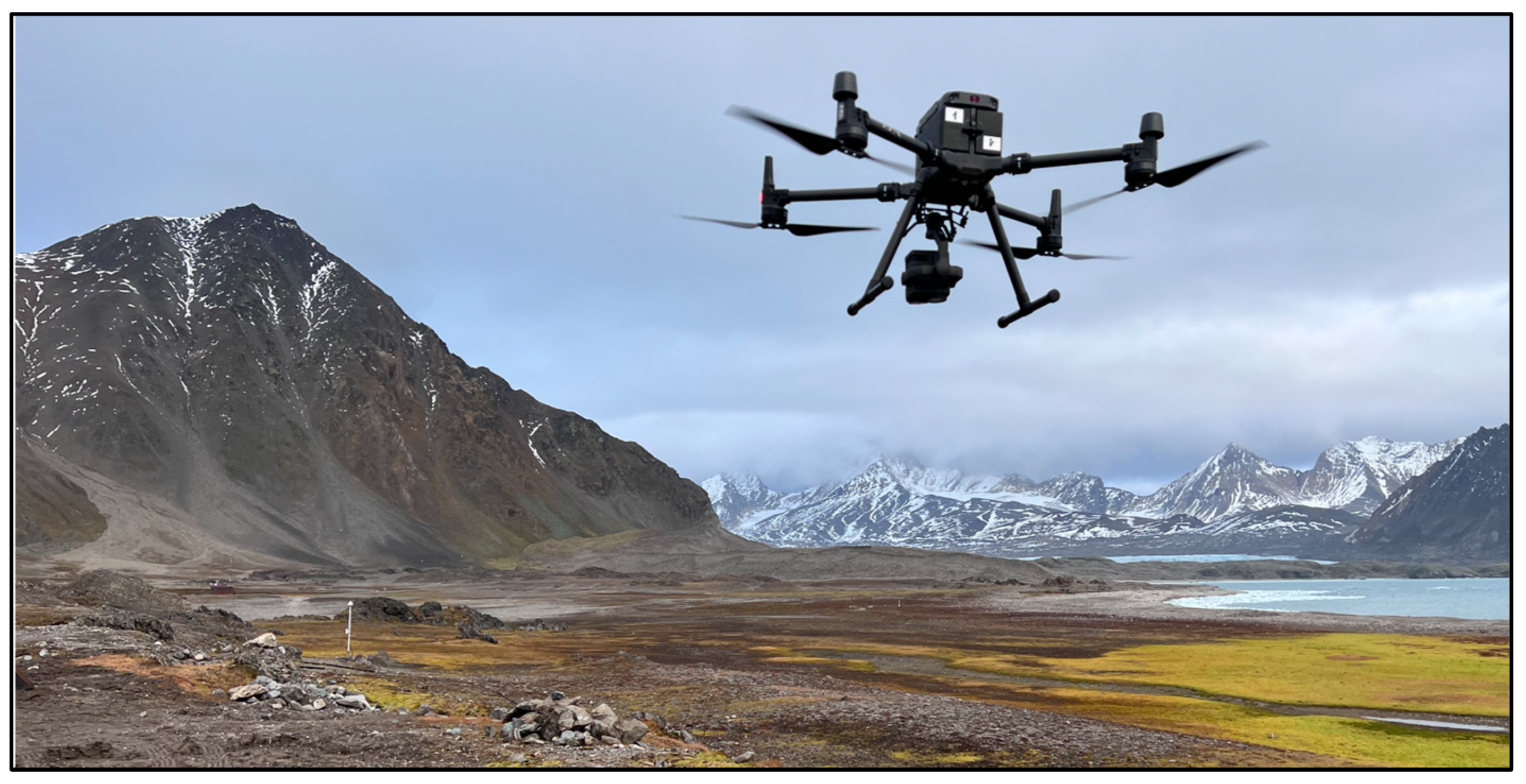
3.1. Drone Missions over Fuglebekken and Ariebekken
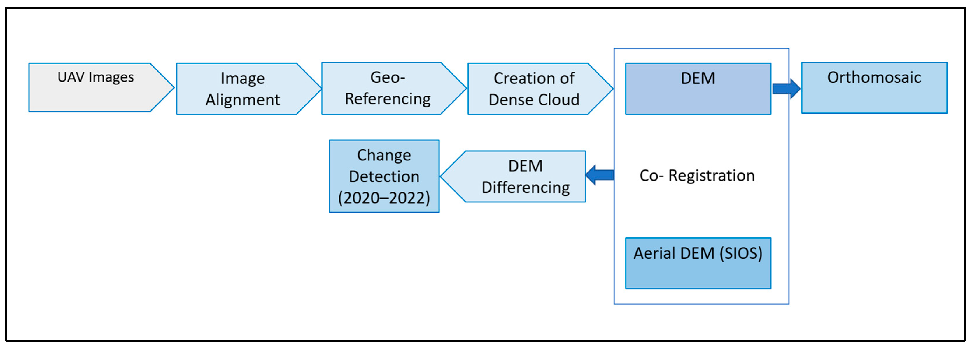
3.2. Data Processing
3.3. Derivation of Catchment Parameters
4. Results
4.1. DEMs and Orthomosaics
4.2. Morphometric Analysis
4.3. DEM Comparisons
4.3.1. Physical Comparisons
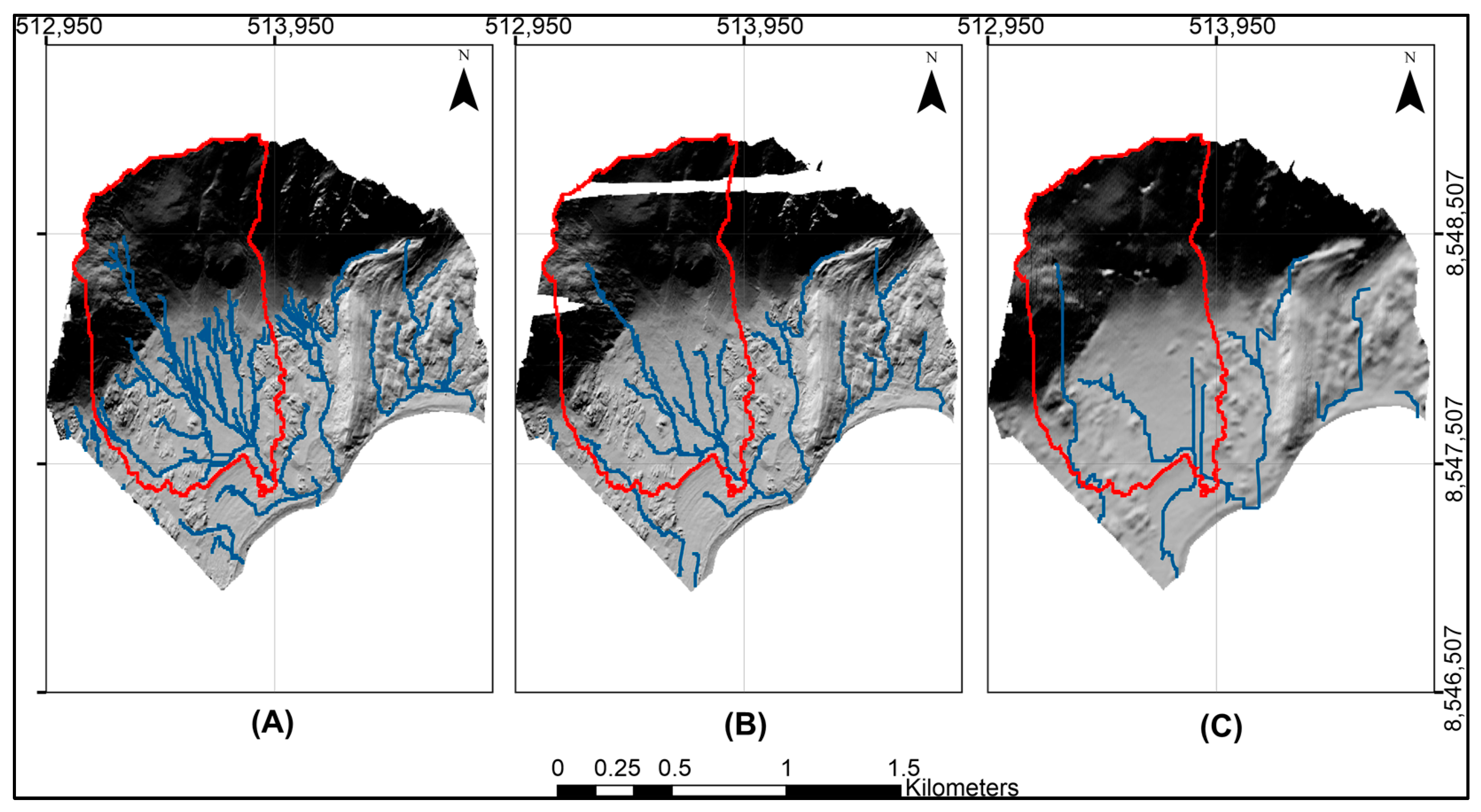
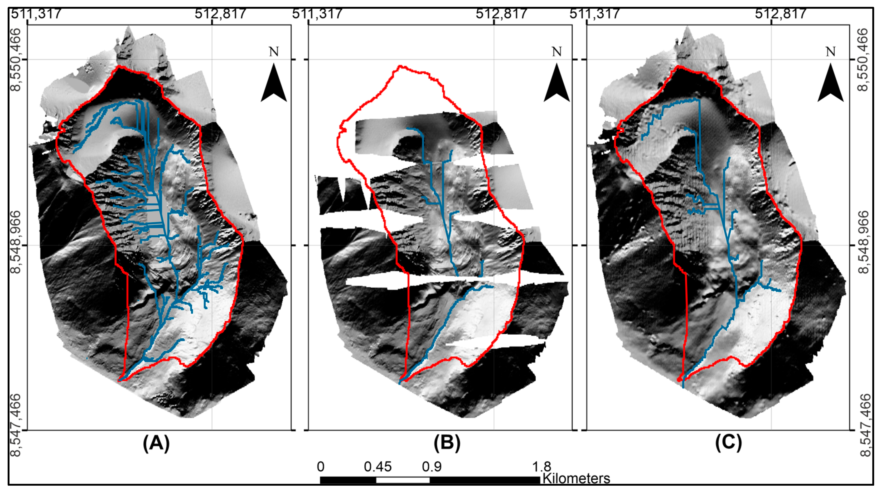
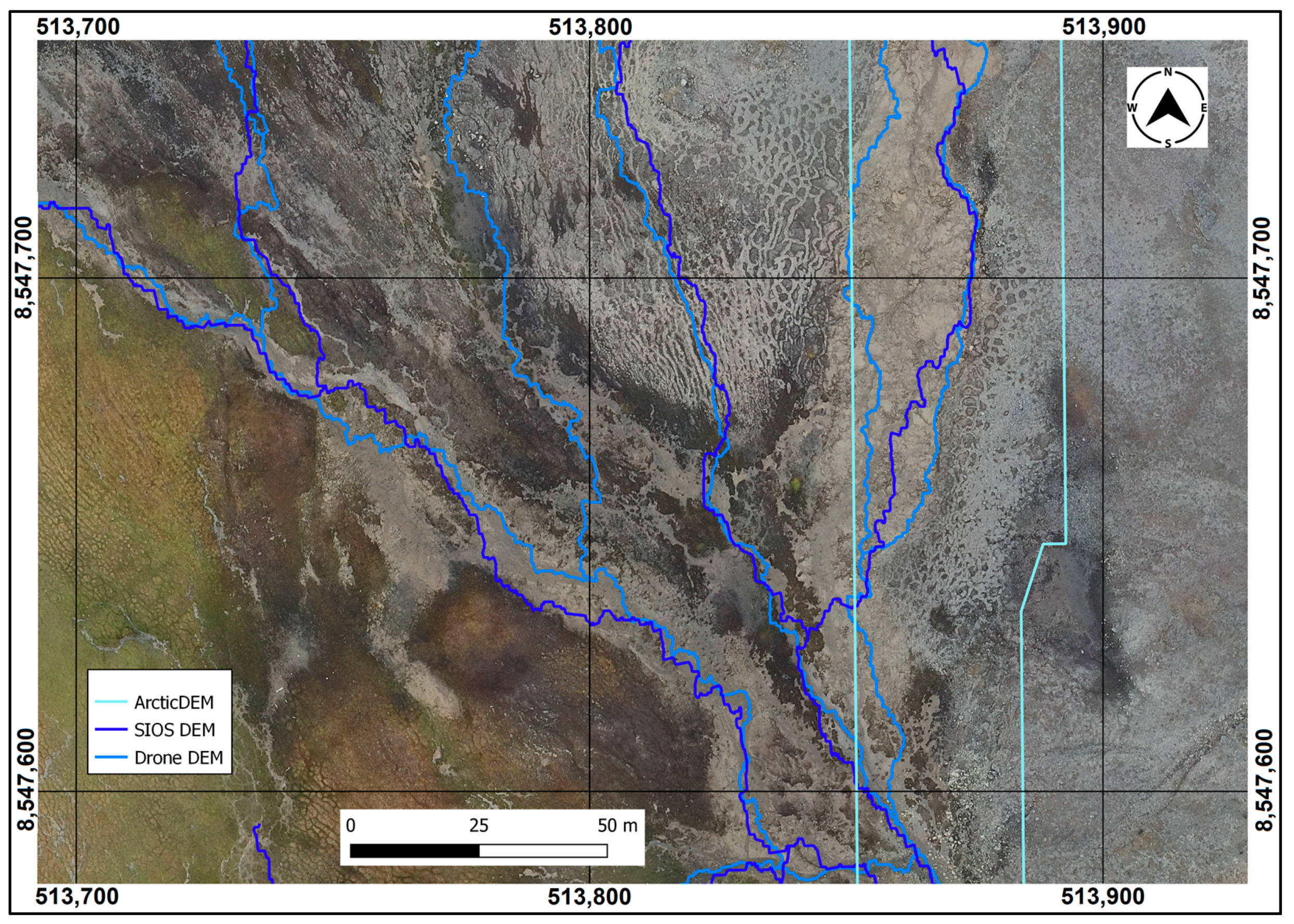
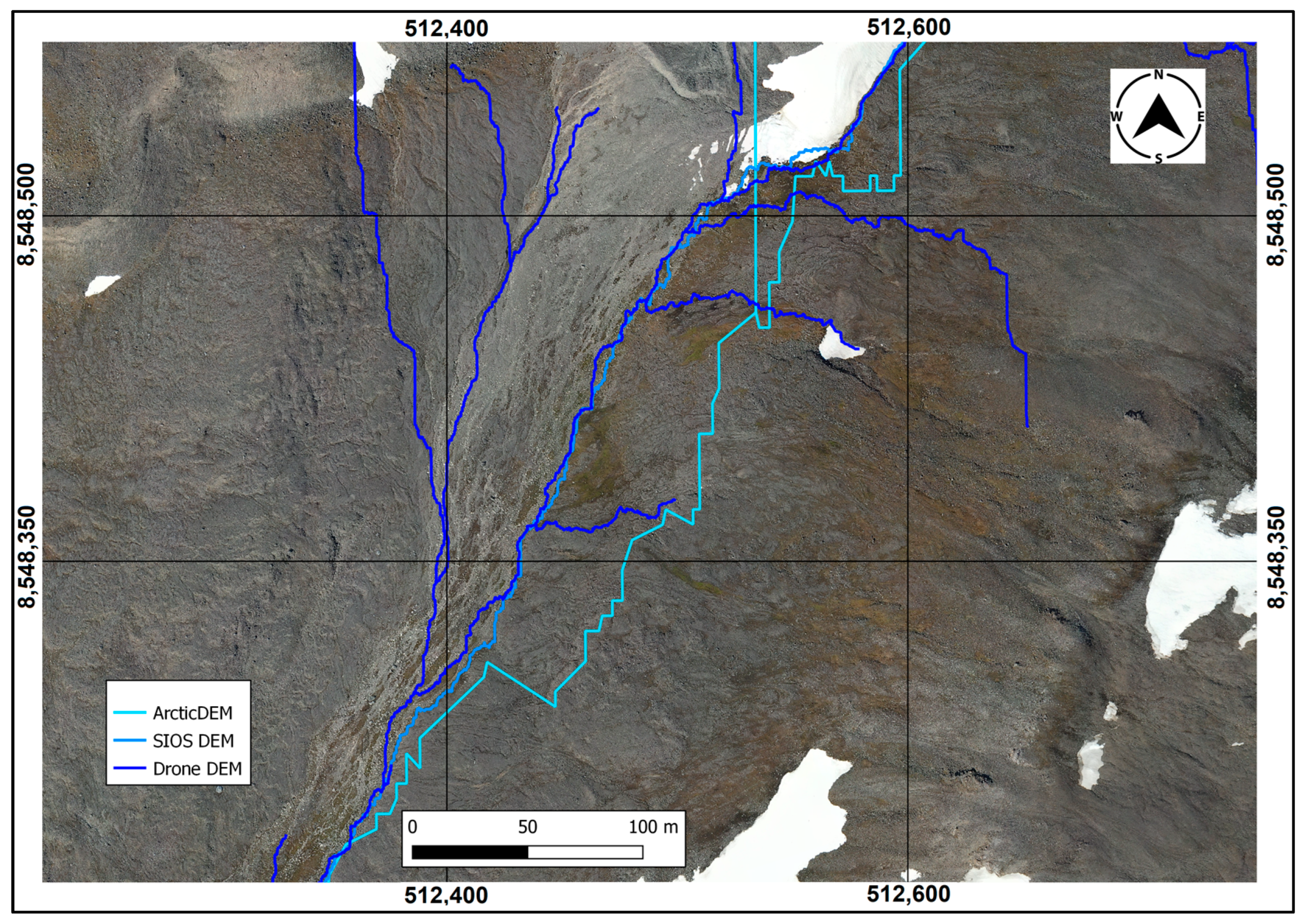
4.3.2. Stream Delineations
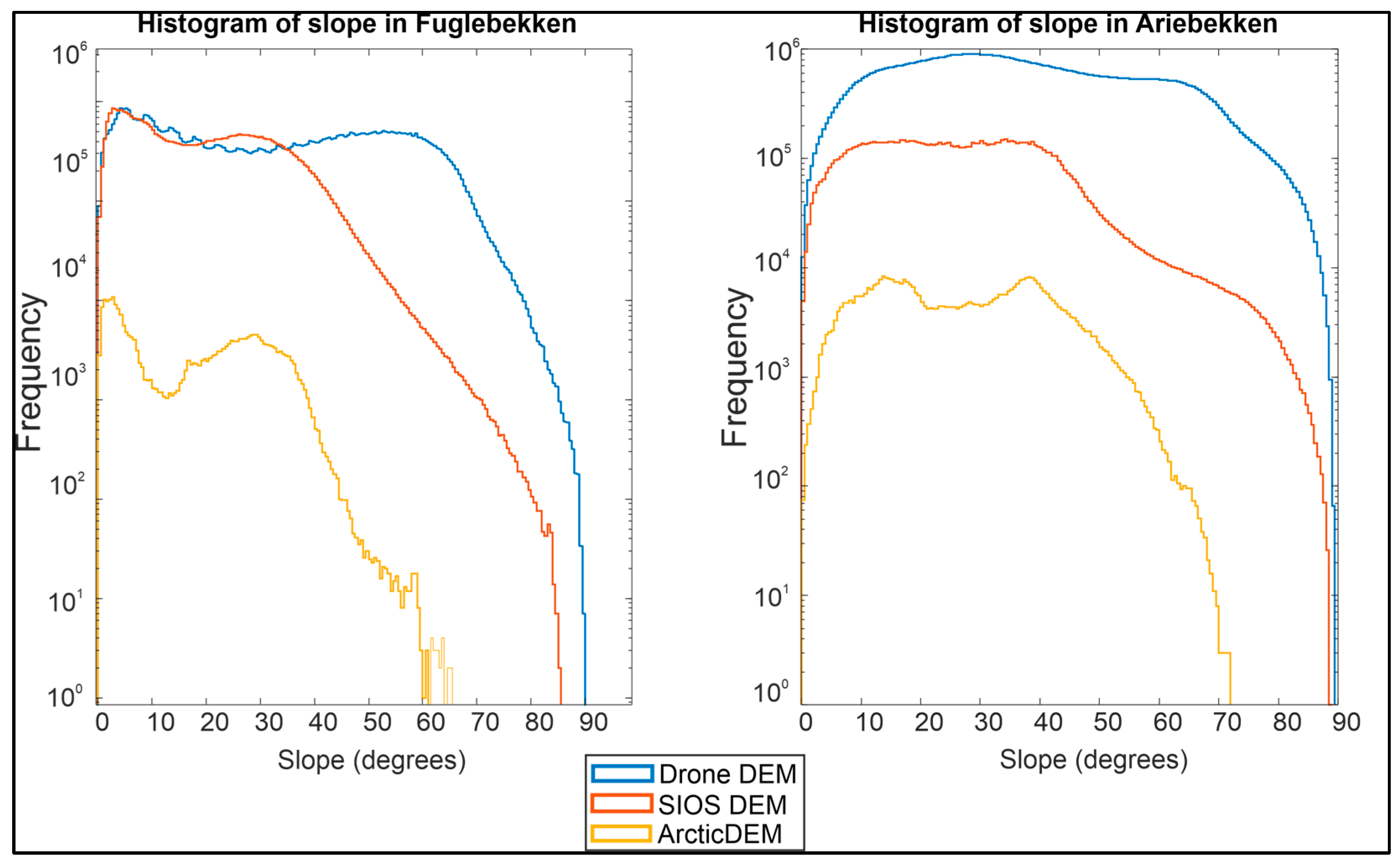
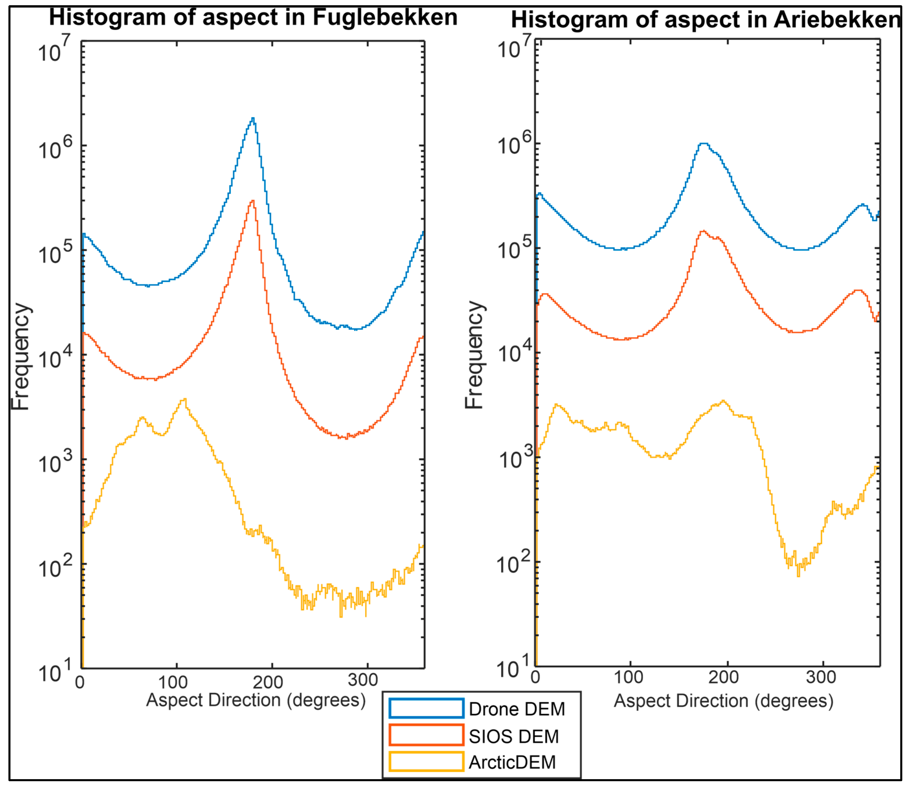
4.3.3. Slope and Aspect
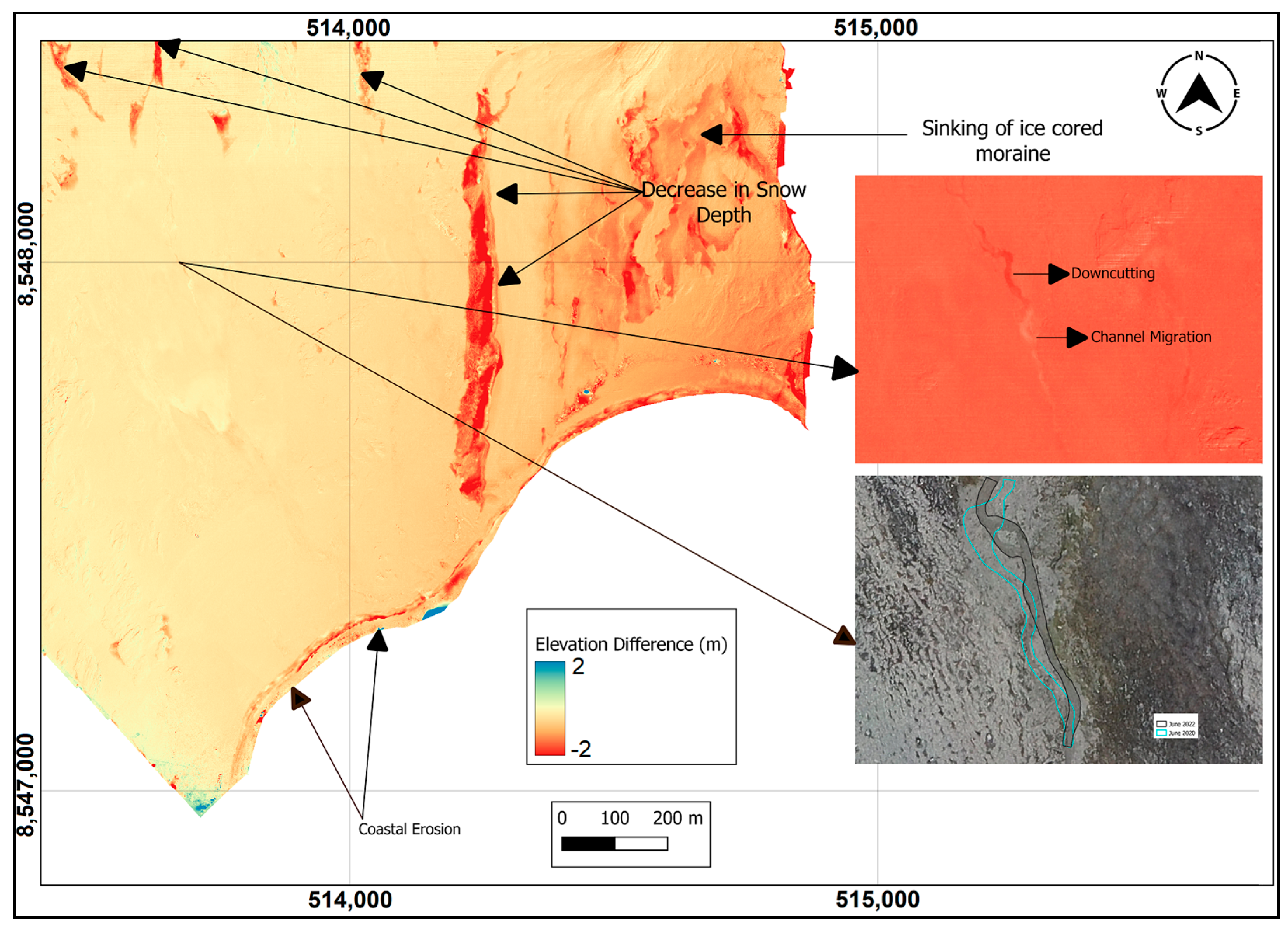
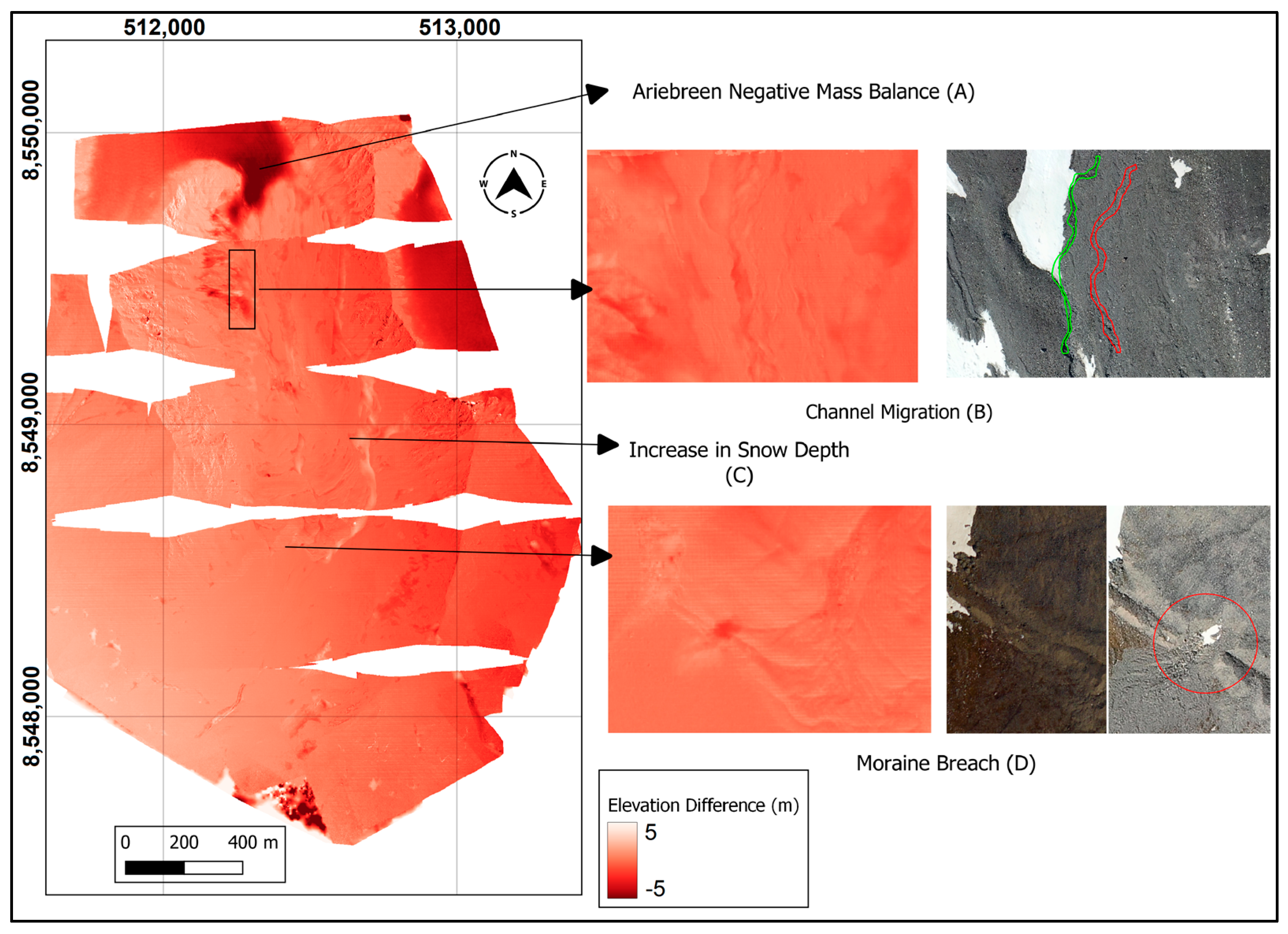
4.4. Change Detection
5. Discussion
6. Conclusions
Author Contributions
Funding
Data Availability Statement
Acknowledgments
Conflicts of Interest
References
- Wawrzyniak, T.; Osuch, M. A 40-year High Arctic climatological dataset of the Polish Polar Station Hornsund (SW Spitsbergen, Svalbard). Earth Syst. Sci. Data 2020, 12, 805–815. [Google Scholar] [CrossRef]
- Meredith, M.; Sommerkorn, M.; Cassotta, S.; Derksen, C.; Ekaykin, A.; Hollowed, A.; Kofinas, G.; Mackintosh, A.; Melbourne-Thomas, J.; Muelbert, M.M.C.; et al. (Eds.) Chapter 3—Polar Regions; Cambridge University Press: Cambridge, UK; New York, NY, USA, 2019; pp. 203–320. [Google Scholar] [CrossRef]
- Masson-Delmotte, V.; Zhai, P.; Pirani, A.; Connors, S.L.; Péan, C.; Berger, S.; Caud, N.; Chen, Y.; Goldfarb, L.; Gomis, M.I.; et al. (Eds.) IPCC: Climate Change 2021: The Physical Science Basis. Contribution of Working Group I to the Sixth Assessment Report of the Intergovernmental Panel on Climate Change; Cambridge University Press: Cambridge, UK; New York, NY, USA, 2021. [Google Scholar] [CrossRef]
- Matti, B.; Dahlke, H.E.; Lyon, S.W. On the Variability of Cold Region Flooding. J. Hydrol. 2016, 534, 669–679. [Google Scholar] [CrossRef]
- Osuch, M.; Wawrzyniak, T.; Łepkowska, E. Changes in the Flow Regime of High Arctic Catchments with Different Stages of Glaciation, SW Spitsbergen. Sci. Total Environ. 2022, 817, 152924. [Google Scholar] [CrossRef]
- Vaze, J.; Teng, J.; Spencer, G. Impact of DEM accuracy and resolution on topographic indices. Environ. Model. Softw. 2010, 25, 1086–1098. [Google Scholar] [CrossRef]
- Błaszczyk, M.; Ignatiuk, D.; Grabiec, M.; Kolondra, L.; Laska, M.; Decaux, L.; Jania, J.; Berthier, E.; Luks, B.; Barzycka, B. Quality Assessment and Glaciological Applications of Digital Elevation Models Derived from Space-Borne and Aerial Images over Two Tidewater Glaciers of Southern Spitsbergen. Remote Sens. 2019, 11, 1121. [Google Scholar] [CrossRef]
- Śledź, S.; Ewertowski, M.W.; Piekarczyk, J. Applications of unmanned aerial vehicle (UAV) surveys and Structure from Motion photogrammetry in glacial and periglacial geomorphology. Geomorphology 2021, 378, 107620. [Google Scholar] [CrossRef]
- Hann, R.; Altstädter, B.; Betlem, P.; Deja, K.; Dragańska-Deja, K.; Ewertowski, M.; Hartvich, F.; Jonassen, M.; Lampert, A.; Laska, M.; et al. Scientific Applications of Unmanned Vehicles in Svalbard (UAV Svalbard). In SESS report 2020—The State of Environmental Science in Svalbard—An annual report. Svalbard Integr. Arct. Earth Obs. Syst. 2021, 3, 78–103. [Google Scholar] [CrossRef]
- Gaffey, C.; Bhardwaj, A. Applications of unmanned aerial vehicles in cryosphere: Latest advances and prospects. Remote Sens. 2020, 12, 948. [Google Scholar] [CrossRef]
- Hann, R.; Betlem, P.; Deja, K.; Hartvich, F.; Jonassen, M.; Lampert, A.; Laska, M.; Sobota, I.; Storvold, R.; Zagórski, P. Update to Scientific Applications of Unmanned Vehicles in Svalbard (UAV Svalbard Update). In Svalbard Integrated Arctic Earth Observing System Place: Longyearbyen ISBN Book title: SESS report 2021—The State of Environmental Science in Svalbard—An annual report. Svalbard Integr. Arct. Earth Obs. Syst. 2022, 4, 74–86. [Google Scholar] [CrossRef]
- Claire, P.; Paul, M.; Ian, H.; Myoung-Jon, N.; Brian, B.; Kenneth, P.; Scott, K.; Matthew, S.; Judith, G.; Karen, T.; et al. “ArcticDEM, Version 3”, Harvard Dataverse, V1. 2018. Available online: https://dataverse.harvard.edu/dataset.xhtml?persistentId=doi:10.7910/DVN/OHHUKH (accessed on 1 August 2022).
- Błaszczyk, M.; Laska, M.; Sivertsen, A.; Jawak, S.D. Combined Use of Aerial Photogrammetry and Terrestrial Laser Scanning for Detecting Geomorphological Changes in Hornsund, Svalbard. Remote Sens. 2022, 14, 601. [Google Scholar] [CrossRef]
- Wawrzyniak, T.; Majerska, M.; Osuch, M. Hydrometeorological Dataset (2014–2019) from the High Arctic Unglaciated Catchment Fuglebekken (Svalbard). Hydrol. Process. 2021, 35, e13974. [Google Scholar] [CrossRef]
- Osuch, M.; Wawrzyniak, T.; Majerska, M. Changes in hydrological regime in High Arctic non-glaciated catchment in 1979–2020 using a multimodel approach. Adv. Clim. Chang. Res. 2022, 13, 517–530. [Google Scholar] [CrossRef]
- Zenmuse P1—Full-Frame Aerial Surveying. DJI. (n.d.). Available online: https://www.dji.com/pl/zenmuse-p1 (accessed on 15 November 2022).
- Sanz-Ablanedo, E.; Chandler, J.H.; Rodríguez-Pérez, J.R.; Ordóñez, C. Accuracy of unmanned aerial vehicle (UAV) and SfM photogrammetry survey as a function of the number and location of ground control points used. Remote Sens. 2018, 10, 1606. [Google Scholar] [CrossRef]
- Karušs, J.; Lamsters, K.; Ješkins, J.; Sobota, I.; Džeriņš, P. UAV and GPR Data Integration in Glacier Geometry Reconstruction: A Case Study from Irenebreen, Svalbard. Remote Sens. 2022, 14, 456. [Google Scholar] [CrossRef]
- Küng, O.; Strecha, C.; Beyeler, A.; Zufferey, J.-C.; Floreano, D.; Fua, P.; Gervaix, F. The accuracy of automatic photogrammetric techniques on ultra-light UAV imagery. In Proceedings of the UAV-g 2011—Unmanned Aerial Vehicle in Geomatics, Zürich, Switzerland, 14–16 September 2011. [Google Scholar] [CrossRef]
- López-Ramos, A.; Medrano-Barboza, J.P.; Martínez-Acosta, L.; Acuña, G.J.; Remolina López, J.F.; López-Lambraño, A.A. Assessment of Morphometric Parameters as the Basis for Hydrological Inferences in Water Resource Management: A Case Study from the Sinú River Basin in Colombia. ISPRS Int. J. Geo-Inf. 2022, 11, 459. [Google Scholar] [CrossRef]
- Boonklong, O.; Jaroensutasinee, M.; Jaroensutasinee, K. Computation of D8 Flow Line at Ron Phibun Area, Nakhon Si Thammarat, Thailand. World Acad. Sci. Eng. Technol. 2007, 33, 1–4. [Google Scholar]
- Jiménez-Jiménez, S.I.; Ojeda-Bustamante, W.; Marcial-Pablo, M.D.J.; Enciso, J. Digital terrain models generated with low-cost UAV photogrammetry: Methodology and accuracy. ISPRS Int. J. Geo-Inf. 2021, 10, 285. [Google Scholar] [CrossRef]
- Skrzypek, G.; Wojtuń, B.; Richter, D.; Jakubas, D.; Wojczulanis-Jakubas, K.; Samecka, A. Diversification of Nitrogen Sources in Various Tundra Vegetation Types in the High Arctic. PLoS ONE 2015, 10, e0136536. [Google Scholar] [CrossRef]
- Noh, M.J.; Howat, I.M. The Surface Extraction from TIN Based Search-Space Minimization (SETSM) Algorithm. ISPRS J. Photogramm. Remote Sens. 2017, 129, 55–76. [Google Scholar] [CrossRef]
- Buakhao, W.; Kangrang, A. DEM resolution impact on the estimation of the physical characteristics of watersheds by using SWAT. Adv. Civ. Eng. 2016, 2016, 8180158. [Google Scholar] [CrossRef]
- Adakudlu, M.; Andersen, J.; Bakke, J.; Beldring, S.; Benestad, R.; Bilt, W.V.D.; Bogen, J.; Borstad, C.; Breili, K.; Breivik, Ø.; et al. Climate in Svalbard 2100—A Knowledge Base for Climate Adaptation. 2019. Available online: https://repository.oceanbestpractices.org/handle/11329/1382 (accessed on 5 September 2022).
- Marciniak, A.; Osuch, M.; Wawrzyniak, T.; Owoc, B.; Dobiński, W.; Glazer, M.; Majdański, M. Multi-method geophysical mapping of ground properties and periglacial geomorphology in Hans Glacier forefield, SW Spitsbergen. Pol. Polar Res. 2022, 43/2, 101–123. [Google Scholar] [CrossRef]
- Lamsters, K.; Ješkins, J.; Sobota, I.; Karušs, J.; Džeriņš, P. Surface Characteristics, Elevation Change, and Velocity of High-Arctic Valley Glacier from Repeated High-Resolution UAV Photogrammetry. Remote Sens. 2022, 14, 1029. [Google Scholar] [CrossRef]
- Etzelmüller, B.; Björnsson, H. Map analysis techniques for glaciological applications. Int. J. Geogr. Inf. Sci. 2022, 14, 567–581. [Google Scholar] [CrossRef]
- Rippin, D.; Willis, I.; Arnold, N.; Hodson, A.; Moore, J.; Kohler, J.; Björnsson, H. Changes in geometry and subglacial drainage of Midre Lovénbreen, Svalbard, determined from digital elevation models. Earth Surf. Process. Landf. J. Br. Geomorphol. Res. Group 2003, 28, 273–298. [Google Scholar] [CrossRef]
- Pope, A.; Murray, T.; Luckman, A. DEM quality assessment for quantification of glacier surface change. Ann. Glaciol. 2007, 46, 189–194. [Google Scholar] [CrossRef]
- Lousada, M.; Pina, P.; Vieira, G.; Bandeira, L.; Mora, C. Evaluation of the use of very high resolution aerial imagery for accurate ice-wedge polygon mapping (Adventdalen, Svalbard). Sci. Total Environ. 2018, 615, 1574–1583. [Google Scholar] [CrossRef]
- Karušs, J.; Lamsters, K.; Sobota, I.; Ješkins, J.; Džeriņš, P.; Hodson, A. Drainage system and thermal structure of a High Arctic polythermal glacier: Waldemarbreen, western Svalbard. J. Glaciol. 2021, 68, 591–604. [Google Scholar] [CrossRef]
- Hodson, A.; Anesio, A.M.; Ng, F.; Watson, R.; Quirk, J.; Irvine-Fynn, T.; Dye, A.; Clark, C.; McCloy, P.; Kohler, J.; et al. A glacier respires: Quantifying the distribution and respiration CO2 flux of cryoconite across an entire Arctic supraglacial ecosystem. J. Geophys. Res. Biogeosciences 2007, 112, 1–9. [Google Scholar] [CrossRef]
- Rippin, D.M.; Pomfret, A.; King, N. High resolution mapping of supra-glacial drainage pathways reveals link between micro-channel drainage density, surface roughness and surface reflectance. Earth Surf. Process. Landf. 2015, 40, 1279–1290. [Google Scholar] [CrossRef]
- Whitehead, K.; Moorman, B.J.; Hugenholtz, C.H. Brief Communication: Low-cost, on-demand aerial photogrammetry for glaciological measurement. Cryosphere 2013, 7, 1879–1884. [Google Scholar] [CrossRef]
- Kraaijenbrink, P.; Meijer, S.W.; Shea, J.M.; Pellicciotti, F.; De Jong, S.M.; Immerzeel, W.W. Seasonal surface velocities of a Himalayan glacier derived by automated correlation of unmanned aerial vehicle imagery. Ann. Glaciol. 2016, 57, 103–113. [Google Scholar] [CrossRef]
- Parizi, E.; Khojeh, S.; Hosseini, S.M.; Moghadam, Y.J. Application of Unmanned Aerial Vehicle DEM in flood modeling and comparison with global DEMs: Case study of Atrak River Basin, Iran. J. Environ. Manag. 2022, 317, 115492. [Google Scholar] [CrossRef]
- Gaffey, C.B.; Bhardwaj, A.; Frey, K.E.; Estes, L. Polar and Cryospheric Remote Sensing Using sUAS. In sUAS Applications in Geography. Geotechnologies and the Environment; Konsoer, K., Leitner, M., Lewis, Q., Eds.; Springer: Cham, Switzerland, 2022; Volume 24. [Google Scholar] [CrossRef]
- Ewertowski, M.W.; Tomczyk, A.M.; Evans, D.J.A.; Roberts, D.H.; Ewertowski, W. Operational Framework for Rapid, Very-high Resolution Mapping of Glacial Geomorphology Using Low-cost Unmanned Aerial Vehicles and Structure-from-Motion Approach. Remote Sens. 2019, 11, 65. [Google Scholar] [CrossRef]
- Carrivick, J.L.; Heckmann, T. Short-term geomorphological evolution of proglacial systems. Geomorphology 2017, 287, 3–28. [Google Scholar] [CrossRef]
- SESS UAV Database. Database of Scientific Applications of Unmanned Vehicles in Svalbard; Version 1; Zenodo Dataset: Meyrin, Switzerland, 2021. [Google Scholar] [CrossRef]
- Berthling, I.; Berti, C.; Mancinelli, V.; Stendardi, L.; Piacentini, T.; Miccadei, E. Analysis of the paraglacial landscape in the Ny-Ålesund area and Blomstrandøya (Kongsfjorden, Svalbard, Norway). J. Maps 2020, 16, 818–833. [Google Scholar] [CrossRef]
- Ewertowski, M.W.; Tomczyk, A.M. Reactivation of temporarily stabilized ice-cored moraines in front of polythermal glaciers: Gravitational mass movements as the most important geomorphological agents for the redistribution of sediments (a case study from Ebbabreen and Ragnarbreen, Svalbard). Geomorphology 2020, 350, 106952. [Google Scholar] [CrossRef]
- De Haas, T.; Kleinhans, M.G.; Carbonneau, P.E.; Rubensdotter, L.; Hauber, E. Surface morphology of fans in the high-Arctic periglacial environment of Svalbard: Controls and processes. Earth-Sci. Rev. 2015, 146, 163–182. [Google Scholar] [CrossRef]
- Tonkin, T.N.; Midgley, N.G.; Cook, S.J.; Graham, D.J. Ice-cored moraine degradation mapped and quantified using an unmanned aerial vehicle: A case study from a polythermal glacier in Svalbard. Geomorphology 2016, 258, 1–10. [Google Scholar] [CrossRef]
- James, M.R.; Chandler, J.H.; Eltner, A.; Fraser, C.; Miller, P.E.; Mills, J.P.; Noble, T.; Robson, S.; Lane, S.N. Guidelines on the use of structure-from-motion photogrammetry in geomorphic research. Earth Surf. Process. Landf. 2019, 44, 2081–2084. [Google Scholar] [CrossRef]


| Parameter | Formula | Ariebekken | Fuglebekken | |
|---|---|---|---|---|
| Areal Parameters | Basin Area (Ab) | Area of the basin (km2) | 2.117 | 1.401 |
| Basin Perimeter (P) | Perimeter of the basin (km) | 8.543 | 6.598 | |
| Basin Length (Lb) | Maximum length of the basin (km) | 2.55 | 1.807 | |
| Form Factor (Ff) | Ff = (Ab/Lb2) | 0.326 | 0.429 | |
| Circulatory Ratio (Rc) | Rc = Ab/((P2)/(4π)) | 0.364 | 0.241 | |
| Elongation Ratio (Re) | Re = Dc/Lb Dc—Diameter of a circle having the same area as the basin | 0.644 | 0.738 | |
| Relief Parameters | Basin Relief (H) | H = Hmax − Hmin (m) | 633.04 | 508.71 |
| Relief Ratio (Rr) | Rr = H/Lb | 0.248 | 0.280 | |
| Average Slope | Average slope of the basin (degrees) | 40.92 | 32.07 |
| Drone DEM | SIOS DEM | ArcticDEM | |
|---|---|---|---|
| Platform | Drone | Aeroplane | Satellite |
| Sensor | Zenmuse P1 35 mm | Phasone IXU-150, Schneider LS 55 mm | Various |
| Acquisition Date | 25 June 2022 (Fuglebekken) 2 July 2022 (Ariebekken) | 22 June 2020 | Created on 23 July 2018 (mosaic of 49 strips acquired between 2013 and 2017) |
| Spatial Resolution | 0.06 m (Fuglebekken) 0.07 m (Ariebekken) | 0.169 m | 2 m |
Disclaimer/Publisher’s Note: The statements, opinions and data contained in all publications are solely those of the individual author(s) and contributor(s) and not of MDPI and/or the editor(s). MDPI and/or the editor(s) disclaim responsibility for any injury to people or property resulting from any ideas, methods, instructions or products referred to in the content. |
© 2023 by the authors. Licensee MDPI, Basel, Switzerland. This article is an open access article distributed under the terms and conditions of the Creative Commons Attribution (CC BY) license (https://creativecommons.org/licenses/by/4.0/).
Share and Cite
Alphonse, A.B.; Wawrzyniak, T.; Osuch, M.; Hanselmann, N. Applying UAV-Based Remote Sensing Observation Products in High Arctic Catchments in SW Spitsbergen. Remote Sens. 2023, 15, 934. https://doi.org/10.3390/rs15040934
Alphonse AB, Wawrzyniak T, Osuch M, Hanselmann N. Applying UAV-Based Remote Sensing Observation Products in High Arctic Catchments in SW Spitsbergen. Remote Sensing. 2023; 15(4):934. https://doi.org/10.3390/rs15040934
Chicago/Turabian StyleAlphonse, Abhishek Bamby, Tomasz Wawrzyniak, Marzena Osuch, and Nicole Hanselmann. 2023. "Applying UAV-Based Remote Sensing Observation Products in High Arctic Catchments in SW Spitsbergen" Remote Sensing 15, no. 4: 934. https://doi.org/10.3390/rs15040934
APA StyleAlphonse, A. B., Wawrzyniak, T., Osuch, M., & Hanselmann, N. (2023). Applying UAV-Based Remote Sensing Observation Products in High Arctic Catchments in SW Spitsbergen. Remote Sensing, 15(4), 934. https://doi.org/10.3390/rs15040934