Globally vs. Locally Trained Machine Learning Models for Landslide Detection: A Case Study of a Glacial Landscape

Abstract

Landslide risk mitigation is limited by data scarcity; however, this could be improved using continuous landslide detection systems. To investigate which image types and machine learning models are most useful for landslide detection in a Norwegian setting, we compared the performance of five different machine learning models, for the Jølster case study (30 July 2019), in Western Norway. These included three globally pre-trained models; (i) the continuous change detection and classification (CCDC) algorithm, (ii) a combined k-means clustering and random forest classification model, and (iii) a convolutional neural network (CNN), and two locally trained models, including; (iv) classification and regression Trees and (v) a U-net CNN model. Images used included Sentinel-1, Sentinel-2, as well as digital elevation model (DEM) and slope. The globally trained models performed poorly in shadowed areas and were all outperformed by the locally trained models. A maximum Matthew’s correlation coefficient (MCC) score of 89% was achieved with a CNN U-net deep learning model, using combined Sentinel-1 and -2 images as input. This is one of the first attempts to apply deep learning to detect landslides with both Sentinel-1 and -2 images. Using Sentinel-1 images only, the locally-trained deep-learning model significantly outperformed the conventional machine learning model. These findings contribute to developing a national continuous monitoring system for landslides.

1. Introduction

Landslides are the most widespread geologic hazard, yet are amongst the least reported type of disasters. In the period 1998–2017, landslides affected an estimated 4.8 million people globally, resulting in over 18,000 fatalities [1]. Landslides can occur in soil or rock materials and include a variety of slope failure mechanisms such as falls, slides, spreads, and flows [2]. They may occur as single events, or multiple events sharing a common triggering event such as heavy rainfall or an earthquake and occur most frequently in regions with high hydrogeological or seismic hazard [3].

Accurate knowledge of past landslide events is needed to mitigate risk from future events. This knowledge is used to develop an understanding of the local hazard conditions, needed for accurate hazard and susceptibility mapping, spatial planning and landslide early warning systems [4,5]. A lack of systematic information on the type, abundance, and distribution of historic landslides is a major limitation for landslide risk mitigation.

Landslides are generally detected from field observations or remotely sensed imagery [5]. There have been an increasing number of studies investigating automated methods for landslide detection and mapping using machine learning models and satellite images, particularly since 2017 [6]. Operational monitoring and alert systems using similar approaches exist for deforestation [7,8,9] and are being developed for other types of natural hazards, including flood [10] and wildfire detection [11,12]. Similar systems for landslide detection would be extremely valuable for obtaining timely and objective data on landslide events. This would lead to an improved understanding of the controlling factors and spatial distribution of past and future landslides and improved reliability of susceptibility and hazard maps [13].

Many of the same change detection methods and data types used for continuous monitoring of forest loss are also relevant for landslide detection, given that landslides often result in the removal of vegetation. Change detection with machine-learning techniques can be performed using temporal or spatial data from satellite images. Temporal methods can detect abrupt changes in time-series data due to a change in ground cover properties. For example, the continuous change detection and classification (CCDC) algorithm [14] can detect gradual and abrupt changes in land cover types. This involves detecting deviances from expected values based on patterns of historic seasonal spectral behavior for a given pixel. The original CCDC model has been run for all existing Landsat data globally, with results made available on Google Earth Engine [15]. We did not find any examples of automated landslide detection using similar time-series-based change detection methods.

Spatial methods on the other hand, are popular for both deforestation and landslide detection. Pixels showing vegetation loss can be identified from post-event, or from sets of pre- and post-event images, using various machine learning methods. Deep learning, and particularly, U-net architecture, has proven to be a powerful segmentation tool in scenarios with limited data, simple structure, and high recognition accuracy. These methods typically follow a workflow that involves training a model using an existing local landslide inventory. The pre-trained model is then used to predict landslides in the surrounding regions that are similar to the training area [16]. Recently U-Net has been widely used in landslide mapping, e.g., [17,18,19,20,21].

In terms of image types used, optical multispectral and LiDAR (light detection and ranging) data are common. However, event detection may be delayed by months due to persistent cloud cover. Hence, there has recently been increasing use of synthetic aperture radar (SAR) data for landslide detection [22,23,24] and continuous monitoring systems for deforestation [7,25,26]. SAR data are also useful for change detection in areas where there are strong seasonal variations, including snow, seasonal darkness, and lack of vegetative biomass (e.g., in temperate and cold climates). Using U-net architecture, a combination of both Sentinel-1 and Sentinel-2 input data, was found to achieve improved accuracy compared to optical data only, for detecting illegal logging events in both summer and winter in Ukraine. The input was stacks of optical and radar images in summer and spring, and radar images only in winter and autumn [27]. However, there are barriers to using SAR data for landslide detection, due to more complicated pre-processing, and a lack of understanding of how to interpret landslides in SAR backscatter data [24]. Therefore, most machine learning models for landslide detection use optical or multispectral images as input data [6].

However, even if cloud-free optical images are available shortly after a triggering event, applying U-Net models for rapid landslide mapping in emergencies is often not feasible. This is the case when there is a lack of historic and local landslide data, represented as polygon features, available to pre-train the model [3]. In response to this problem, there have been attempts to produce globally-trained generalized machine learning models capable of detecting and mapping landslides in previously unseen locations. The first attempt was by Prakash et al. (2021) with a convolutional neural network (CNN) model that was trained on seven locations around the seismically active Pacific Ring, with high vegetation coverage [28]. Another example was by Tehrani et al. (2021), who developed an object-based method using k-means clustering to perform semantic segmentation, followed by random forest classifiers that determine whether the segments represent landslides or not [29]. This model was trained on data from 29 locations around the world.

In this study, our main goal is to determine which elements of existing automatic landslide detection and deforestation monitoring approaches could be feasible to include in a national landslide detection system in Norway. This represents one of the first attempts to use machine learning to detect and map landslides in Norway. With a glacially sculpted landscape with steep slopes, and strong seasonal variability, the environment in Norway is relatively unique, and it is unknown how well the generalized models will perform in such a setting. We investigate the performance of five different machine learning models using satellite images from Sentinel-1 and -2, along with elevation and slope rasters. The well-verified landslide inventory from the Jølster case study (30 July 2019) [30] is used to test which approaches could be adapted for larger-scale use in the future.

We test the performance of three pre-existing globally-trained models, including (i) the time-series-based CCDC algorithm, (ii) the object-based model from Tehrani et al., (2021), and (iii) the pixel-based CNN model from Prakash et al. (2021). Two locally-trained models were also tested, including: (iv) a classification and regression tree (CART) machine learning model [31] and (v) a CNN U-net deep learning model.

The following research questions are investigated:

• How do globally pre-trained machine learning models for landslide detection perform in a glacial landscape?
• Which locally-trained model and input data combination gives the best results?
• Which elements of the investigated models could be implemented in an operational national landslide detection system?

In the following section, we describe the current situation in Norway in terms of landslide hazards and introduce the case study. In the results, we show that the globally trained models generally did not perform well in a glacial landscape, particularly for landslides on north-facing slopes. The locally trained deep learning model outperformed the machine learning model with all input data combinations, except for one. The best performance (MCC score: 89%) was achieved using combined Sentinel-1 and Sentinel-2 data as input. We did not attempt to retrain or modify the existing globally pre-trained models in this study, although we provide suggestions as to how their performance could be improved in the discussions.

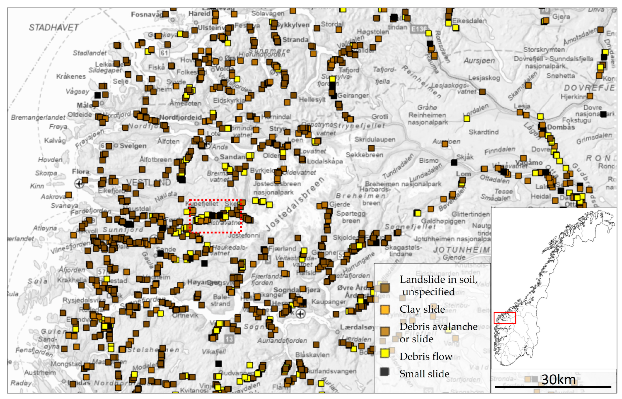
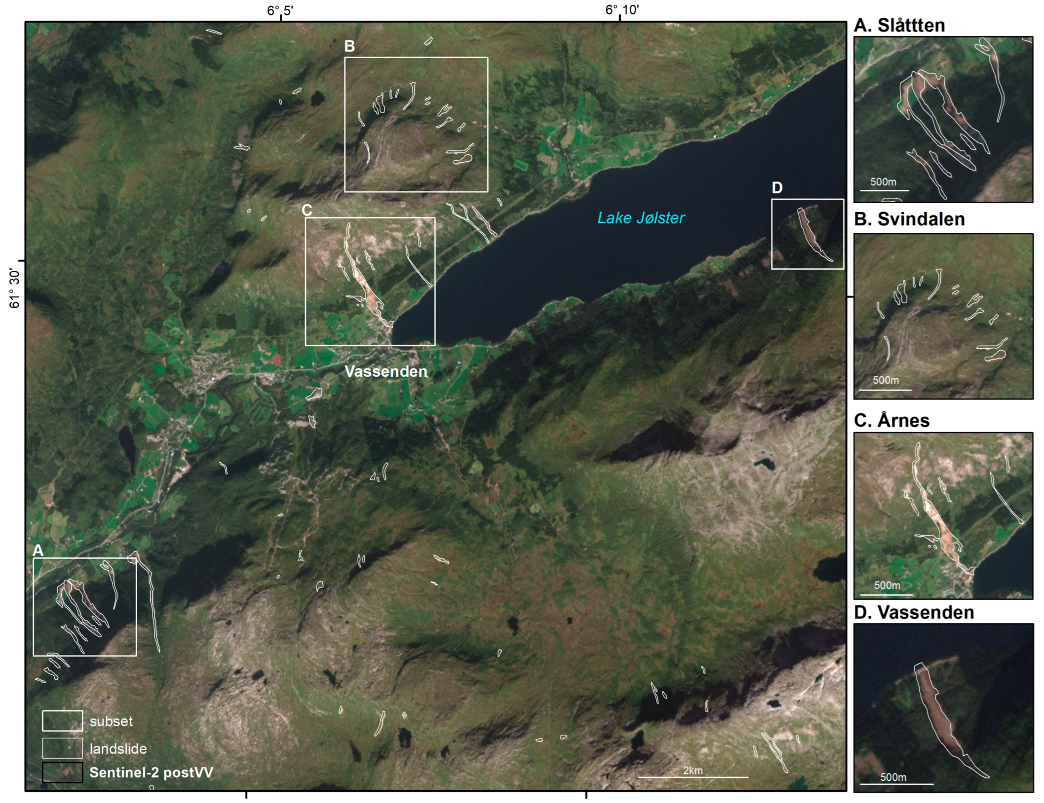
2. Norwegian Setting and Case Study

Landslides occur almost daily in mountainous regions in Norway and are the natural hazard responsible for most fatalities [32]. In addition, they cause large economic losses due to damage to infrastructure and disruption to transportation [33]. In comparison to other countries in Europe, Norway has a relatively high proportion of land area that is susceptible to landslides, with over 70% of municipalities affected [34]. This is due to the geological landscape with high mountains, valleys with steep slopes, and post-glacial isostatic rebound that has resulted in sensitive clays in valley bottoms in coastal regions [32].

The most frequent types of landslides in Norway include rock fall, rock slides, debris avalanches, and debris flows [13]. In addition, there are unstable mountains and deep-seated landslides that can evolve into large rock avalanches and quick clay slides [32].

To mitigate the increasing risk to society due to landslide hazards, there are several national initiatives coordinated by the Norwegian Water Resources and Energy Directorate (NVE). These include, among others, the preparation of susceptibility and hazard maps and close communication with spatial planners at municipalities to protect inhabitants and key infrastructure already located in hazardous areas. NVE is also working with the prediction of hydro-meteorologically induced landslide occurrences through a national early forecasting and warning service [35]. The early warning system allows municipalities and individuals to take timely action to reduce risk, including evacuations and closure of transport routes in areas with high hazards.

These initiatives rely on knowledge of historic landslide occurrence and are limited by the quality and completeness of historic landslide records [13]. The Norwegian Mass Movements Database (available from: https://nedlasting.nve.no/gis/, accessed on 20 December 2022) contained 84,768 reports at the time of writing, from the year 900 to 2022. Yet there are some significant limitations in the existing landslide dataset that make it unsuitable for spatial analyses; for instance, determining statistical relationships between landslide occurrence and the topographical, geological, hydrological, vegetation, or meteorological factors. These include low locational and qualitative (i.e., information on landslide type, size, and trigger) accuracy of older events that have been extracted from historic church and municipality records. These reports are generally limited to events that caused death or destroyed property.

While modern reporting is performed systematically by the road and rail authorities [36], reporting focuses on events that directly impact transport infrastructure. The given locations are typically represented by the point where a landslide impacted the road, and the initiation point is not usually specified. Although these data generally have high spatial and temporal accuracy, there remain some qualitative inaccuracies. Furthermore, compared to 11 other national landslide databases, there is a spatially biased distribution, with many reports located along roads but relatively few events reported in remote areas [37], as illustrated in Figure 1. NVE use aerial and satellite images to manually map polygons representing the landslides and periodically perform quality control of the existing landslide point data. However, detecting and mapping traces of small landslide events across large areas remain a tedious and labor-intensive process [35].

There is a strong need for improved landslide mapping techniques in Norway, which can provide objective and accurate spatial information, and allow the detection of events that occur away from populated areas and transport routes. Recent studies have demonstrated there is great potential to improve the detection of landslides in remote areas using satellite images [30,38].

In July 2019, an extremely heavy rainfall event triggered multiple landslides in the (formerly named) Jølster municipality in Western Norway [38]. The maximum recorded rainfall was 113 mm in 24 h, exceeding the 200-year event magnitude at the two nearest precipitation weather stations, Botnen and Haukedalen, in the neighboring municipality of Førde [39]. The road authority reported 14 landslides on this date, while mapping from Sentinel-2 images detected 120 events, with only 30% being located within 500 m of a road, compared to 100% of those registered by the road authority [30].

The study area is shown in Figure 2. The landscape consists of steep glacial valleys, lakes, and mountains up to 1666 m. The town of Vassenden is located in a tempered climate zone with relatively mild winters and wet summers due to its proximity to the coast. The mean annual precipitation over the past five years is 2800 mm/yr at the Botnen weather station, and temperatures vary from −25 °C to 31 °C, with an annual mean of 5 °C (https://seklima.met.no/, accessed on 27 January 2023). The hydro-meteorologically induced landslides that pose a risk to these areas are expected to become more frequent due to an increase in extreme precipitation events [40].

The bedrock geology is predominantly granitic (banded and augen) orthogneiss and quartz-monzonite. The geomorphology is shaped by old faults and glacial erosion, with a quaternary surface cover typically consisting of highly consolidated moraine material overlying the bedrock, with a looser veneer of colluvium on valley slopes. The surface cover is thin to non-existent at high altitudes and increases to several meters thick in lower areas close to the lake. The vegetation ranges from sparse moss and shrubs or light birch forest at high elevations to spruce forest and agricultural fields lower in the valleys. Roads and built areas are mainly located in the flatter main valleys. The area is very susceptible to landslides due to the steep slopes and wet climate, with over 40 historic landslides recorded in the national database [30].

3. Methods

We compare the performance of five different models: (i–iii) generalized globally trained predictive models (CCDC, Tehrani, and Prakash), (iv) a locally trained supervised machine learning model in Google Earth Engine (GEE) (smile.Cart classifier), and (v) a locally trained pixel-based deep learning model (U-net). For verification of the results, we used a set of 120 manually mapped landslides [30].

3.1. Generalized Globally-Trained Predictive Models

To run the three generalized globally trained predictive models, the steps in the methods and accompanying documentation on GitHub were followed, with some modifications made where necessary. A summary of these methods and any deviations are described here.

(i) CCDC time-series model [15]: The CCDC model results are available for visualization purposes as an app on GEE. The results have been pre-calculated for the Landsat bands (not including NDVI). The SWIR1 band was chosen for the change detection analysis, as this is known to be sensitive to changes in vegetation. The changes within the period 1 July 2019 to 31 August 2019 were displayed for the study area using the app.

(ii) Tehrani machine learning model [29]: Pre-processing of the input data is performed automatically using a script run in GEE [41]. The script takes a table of landslide coordinates and dates, and generates sets of Geotiff images for each point, which are then used as input for the model. Sentinel-2 Level 1C images with low cloud coverage are selected within three months before and after the landslide event date. If no cloud-free images are found in that period, a composite image is made using images from one year. The pre-processing involves the normalization of the images, and the addition of brightness, NDVI, and GNDVI (green-NDVI) bands, and the output is three images for each landslide point; pre-event, post-event, and difference (see Figure 3I). Modifications made to this process included uploading a shapefile to GEE, instead of a Google Fusion table, which has been discontinued. Further, the 10 m resolution Norwegian DEM was used instead of the global 30 m resolution ALOS DEM, because the ALOS DEM does not cover Norway.

The outputs are raster images with labeled segments in KEA file format [42] and a list of the segments that were classified as landslides.

(iii) Prakash CNN deep learning model [16]: The required inputs are three bands (R, G, B) pre- and post-event images, single-band slope, hillshade, DEM, bounding box, and no-data mask rasters. In the accompanying article [16], it was not specified if Sentinel-2 Level 1C or Level-2A products were used. Pre-processing the input images involved selecting a Sentinel-2 image at the landslide location with the lowest cloud cover within one month of the landslide date, clipping to the area of interest, and then manually creating a mask of snow and clouds. Again, we used the Norwegian DEM instead of a global DEM, from which slope and hillshade rasters were created.

Greenest-pixel composite image: One modification to the methodology described in Prakash et al. [16] was to use a greenest-pixel composite as input, as this method can reduce noise from clouds and agriculture. These were produced using one month of images from before and after the landslides, using the S2 cloudless algorithm for cloud filtering and the SCL (scene classification) band for snow filtering. Using the quality mosaic function, a composite image was then created based on NDVI, in which for each pixel—the pixel with the maximum NDVI is taken, along with the corresponding values from the other bands from the same date. This gives a ‘greenest pixel’ composite that is cloud-free and gives the least snow cover and shadow within the specified date range.

3.2. Locally-Trained Machine and Deep Learning Models

(iv) smile.CART machine learning model: Landslide predictions were performed in Google Earth Engine using the ee.Classifier.smileCart algorithm [31], which uses a CART (Classification and Regression Trees) classifier. This involved the following steps.

First, the images were pre-processed. For Sentinel-2, one month of Level-2A images from before and after the event were used to create cloud-filtered, greenest-pixel composites. Cloud filtering was performed using the s2cloudless algorithm to remove cloudy pixels [43]. Greenest-pixel composites were then created from the pre- and post-event image collections, using the quality mosaic function. All bands from the same image the selected pixel with the highest NDVI value was taken from are included in the output. For Sentinel-1, again, one month of images from pre- and post-event were used to create terrain-corrected median composites. The terrain correction was performed using the volumetric scattering model [44]. Then, median composites for VV and VH bands separately were created from each of the pre- and post-event image collections, using both ascending and descending orbit geometries. Finally, the Sentinel-1 and -2 bands were combined, along with elevation and slope, into a single 13-band image.

Secondly, the supervised classification was performed following the tutorial by S. Levick [45]. This involved selecting training points from which to train the classifier—18 points were manually selected in the landslide class, and 112 points were from seven different non-landslide classes (water, snow/ice, bare rock, agriculture, forest, alpine scrub, and urban). Care was taken to sample from diverse slope aspects, elevations, and within shadow areas. The 13-band image was then sampled at each point, and these values were used to train the classifier and perform a classification across the whole image. In addition, classifications were performed using the same points for a 3-band, and 2-band subsets of the full 13-band image, as shown in

Table 1. Input data used in locally trained models for four different settings.

Model Run	No. of Bands	Bands
S1, S2, and DEM	13	Sentinel-1: pre-VV, post-VV, diff-VV, pre-VH, post-VH, diff-VH
		Sentinel-2: post-R, post-G, post-B, post-NIR, dNDVI
		Terrain: elevation, slope
S1 (VV) and S2	3	Sentinel-1: pre-VV, post-VV
		Sentinel-2: dNDVI
S1 (VV) only	2	pre-VV, post-VV
S2 only	5	post-R, post-G, post-B, post-NIR, dNDVI

.

The results were inspected to see if any misclassification was apparent. Then, finally, a binary image of landslide–non-landslide was produced by combing the non-landslide classes, and salt-and-pepper noise was reduced using the focal mode function.

(v) U-net CNN deep learning model: The entire algorithm was implemented in a Jupyter Notebook using ArcPy, Keras, and TensorFlow 2. The chosen model is a scaled-down version of a deep-learning architecture called U-net, for automatic semantic segmentation [46] with Keras implementation. The U-net is a convolutional network architecture for fast, effective, and precise segmentation of images with its symmetric U-shape. U-net has proven to be a powerful segmentation tool in scenarios with limited data, simple structure, and high recognition accuracy. The network is based on the fully convolutional neural network (FCNN) for semantic segmentation [47,48].

The same input dataset was used for the GEE smile.CART model is described in Section 3.2 (Table 1). We exported random samples as classified tiles for all four settings by generating a minimum of 10,000 samples using an Image Analyst license and ArcGIS Pro [49]. The most suitable tile size in our case was 128 × 128 pixels, and stride (the distance to move in the x- and y-directions when creating the next image chips) of 64 × 64, to have 50% overlap in each sample tile. The output was a dataset of classified image tiles, the format primarily used for pixel classification. During the training process, an input image flows through the CNN network that recognizes it with a set of trainable kernels, resulting in a group of feature maps [50]. The dataset was divided into training, validation, and test subsets. The trained model was saved as a ‘Deep Learning Package’ (‘.dlpk’ format), which is the standard format used to deploy deep learning models on the ArcGIS platform and can be used further as a pre-trained model.

3.3. Performance Evaluation

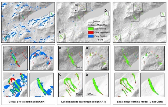
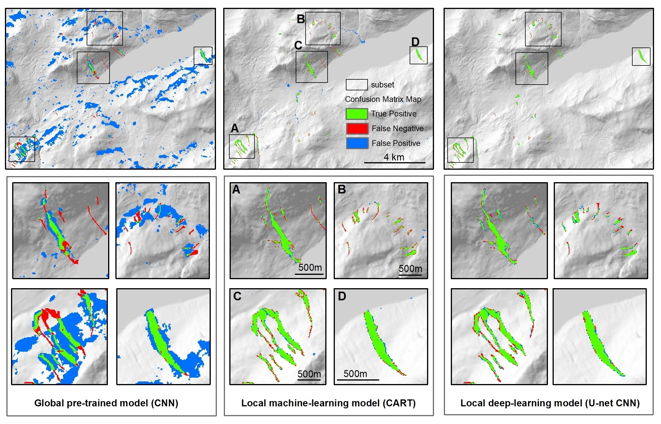
The landslide inventory produced from the Sentinel-2 dNDVI [51] image was used for verifying the results of the other approaches.

Qualitative and quantitative analyses: The results of the CCDC and Tehrani models are briefly described in a qualitative manner, as both these methods produced limited landslide predictions. Additionally, it was not possible to download the CCDC model results from the GEE app; therefore, it was not possible to do quantitative pixel scale analyses on these results.

The Prakash and locally trained modelpredictions were evaluated quantitatively, as follows. The landslide polygons mapped with Sentinel-2 dNDVI were converted to a binary raster of landslide or non-landslide pixels. This was used to validate the automated landslide detection model outputs. Following the approach in ref [16], a map of confusion matrix values was created, showing true positive (TP), false positive (FP), false negative (FN), and true negative (TN) values. From these, the performance metrics precision, recall, F1-score, and MCC scores were calculated (see

Table 2. Equations for performance evaluation metrics from confusion matrix values.

Metric	Formula
Precision	$\frac{TP}{TP+FP}$
Recall	$\frac{TP}{TP+FN}$
F1-score	$\frac{2TP}{2TP+FP+FN}$
MCC	$\frac{TP\times TN-FP\times FN}{\left(TP+FP\right)\left(TP+FN\right)\left(TN+FP\right)\left(TN+FN\right)}$

). Since landslides represent only a tiny fraction of all the pixels in the study area, the learning problem is highly imbalanced towards non-landslide pixels. Therefore, the accuracy score can become unreliable due to the large proportion of true negatives. The MCC score is considered to be the most appropriate metric for comparing the results [52]. For a binary model, the MCC gives a score between 0 to 1, with 0 indicating a model with no correlation (random predictions) and 1 indicating a perfect correlation (all correct predictions).

4. Results

The performance of the three globally-trained and two locally-trained machine learning models in the Jølster case study is presented in this section.

4.1. Globally Trained Models

(i)

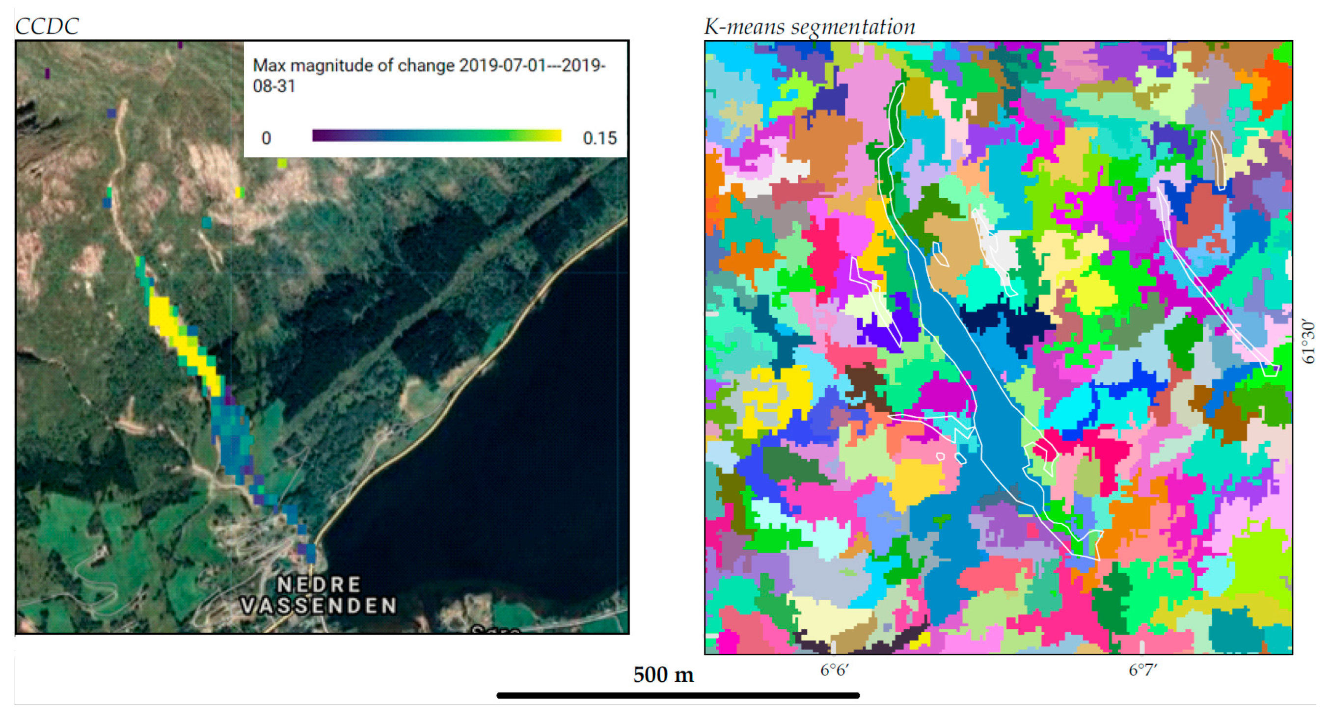
CCDC time-series model:

The CCDC time-series model detected the large Vassenden landslide quite precisely (Figure 4), along with one smaller debris flow to the east. The large landslides at Årnes and Slåtten were not detected, nor were any of the other smaller landslides in the study area.

(ii)

Tehrani machine learning model:

Overall, no landslides were detected using this model. The large landslide at Vassenden was partially segmented (see Figure 4), although the initiation zone was missed, and some nearby fields were included. The deposits of the landslides at Slåtten were also segmented. However, no segments were classified as a landslide.

(iii)

Prakash CNN deep learning model:

The Prakash model was run with three different variations of Sentinel-2 images shown in Figure 3 (1) Level 1C, (2) Level 2A, and (3) a cloud-free greenest-pixel composite. The results are shown as confusion matrix maps in Figure 5. The most striking differences between the runs were firstly, that many false positives (wrongly predicted as a landslide) appear in the Level 2A products, and secondly, in the Level 1C product, there are many false negatives (missed landslides).

After inspecting the results, it was noticed that the false positives in the Level 2A results appeared to be related to unnaturally bright areas on the northern slopes. This turned out to be due to an anomaly resulting from the terrain correction used in processing the Level 2C products, which results in a blueish appearance in shadowed areas in true color composite images and inaccurate surface reflectance values [53]. The problem has been reported to the Sentinel-2 Quality Working Group (December 2021) [54]. An outcome of their analysis is expected in the near future; changes will be reported in the Sentinel 2A Data Quality Report (https://sentinel.esa.int/web/sentinel/user-guides/sentinel-2-msi/document-library, accessed on 15 December 2021). Due to the noise introduced by these artifacts, comparing the performance metrics of the model runs over the entire study area was not very insightful. Therefore, for a more detailed comparison, the metrics were calculated for the sub-plots shown in Figure 5. These are shown in

Table 3. Prakash CNN deep learning model (iii) performance metrics. The metrics were calculated for the entire study area, as well as for the four subplots shown in Figure 5. The model was run with three different input image types; 1. Level-1C images, 2. Level-2A images, and 3. Level-2A images as a cloud-free, greenest pixel composite. The MCC score (Matthew’s Correlation Coefficient) is considered the most representative metric for the imbalanced problem of landslide classification [52].

Location	Input Image	Precision %	Recall %	F1-Score %	MCC %
Entire area	1—S2_L1C	5	4	4	4
	2—S2_L2A	2	45	5	9
	3—S2_L2A_gr	2	37	4	7
A. Slåtten	1—S2_L1C	40	0	0	2
	2—S2_L2A	19	60	29	20
	3—S2_L2A_gr	30	58	40	33
B. Svidalen	1—S2_L1C	86	1	1	8
	2—S2_L2A	6	28	9	8
	3—S2_L2A_gr	8	6	7	5
C. Vassenden	1—S2_L1C	25	17	21	18
	2—S2_L2A	40	51	45	43
	3—S2_L2A_gr	35	46	40	37
D. Årnes	1—S2_L1C	-	0	0	-
	2—S2_L2A	33	96	49	51
	3—S2_L2A_gr	35	60	44	41

.

For the entire study area, the MCC scores are below 1%. In the subplots, there are false positives likely caused by the over-correction artifact in the results for A, B, and D, which are on north-facing slopes. Despite this, the best score was 51% for model Input 2—S2_L2A in subplot D (Årnes landslide). The second best was 43% for model Input 2—S2_L2A in subplot C (Vassenden landslides). Subplots B (Svidalen) and A (Slåtten) had poor results across all runs.

Using Level-1C images, overall, the model failed to detect landslides. Only a small part of the Vassenden landslide was detected. The large landslides on north-facing slopes were not detected at all. There were some false positives, mainly related to changes in agricultural areas. Using Level 2A images (2. single date, and 3. greenest-pixel composite), the model predicted the Vassenden and Årnes landslides fairly well. The landslides in subplot A (Slåtten) were partially detected with the Level-2A images. However, most of the predictions on the steep north-facing slopes are false positives due to noise, while the deposit of the western-most of the three debris flows seems to have been detected meaningfully. It is interesting that that particular deposit was detected, and not the other two, given that from field observations, the deposits of the western-most debris flow were noticeably different from the others. The western-most deposit was a very thin layer of soil, with a high concentration of washed-out light-colored boulders and stones, whereas the other two were much thicker (up to 2 m high) deposits consisting of darker soil and forest debris (seen https://www.nibio.no/nyheter/skogsdrift-ikke-medvirkende-arsak-til-jordras-i-jolster, accessed on 22 December 2022)). In subplot B (Svidalen), there is a significant difference in the number of false positives, with much fewer in the greenest-pixel composite from run 3, compared to run 2. Again, it is not clear if this difference is due to the artifacts or pre-processing. There appears to be just one pixel that has been correctly identified in all three runs. However, overall, the model was not able to detect the smaller landslides. In subplot C (Vassenden), there are more false positives using the greenest-pixel composite in agricultural areas than the single date image. These results are more likely to be meaningful because the slope is south-facing and not affected by the over-correction artifacts. Finally, in subplot D (Årnes), there are slight differences in the number of false positives between the two input image types; however, it is difficult to say whether the difference is related to the artifacts or to the difference between the manually masked image (single date), and the greenest-pixel composite.

The mediocre performance in these model runs is mainly due to introduced image artifacts in shadowed areas, thererfore we find the Prakash CNN deep-learning model is worth further investigation for use in an operational landslide detection system. With different adjustments, such as using input images without the over-corrected shadow areas and including NDVI or Sentinel-1 bands, to make the classification more robust in shadowed areas, the model performance could likely be improved.

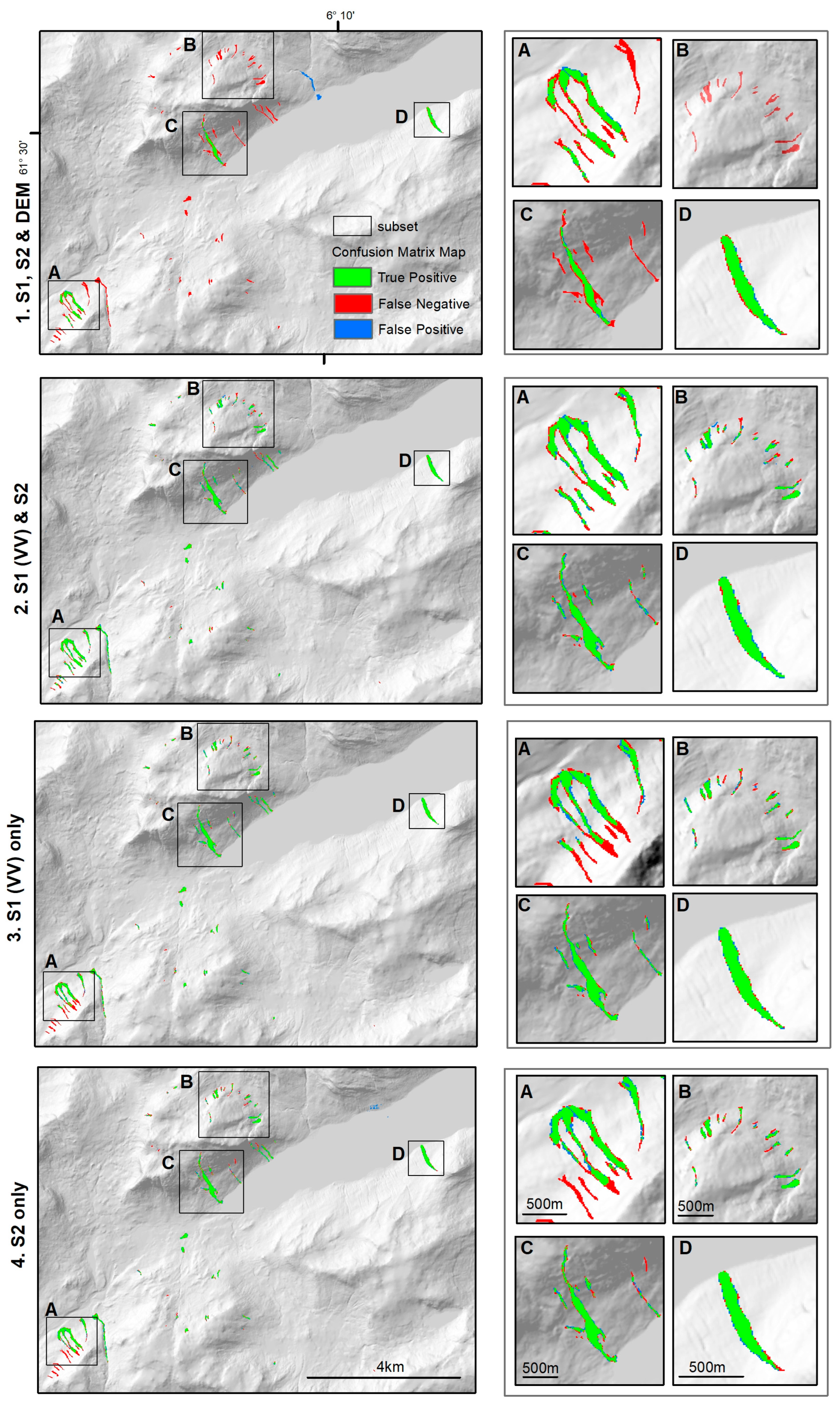
4.2. Locally Trained Models

(iv)

smile.CART machine learning model:

The supervised machine learning model in GEE using the ee.smile.Cart classifier was tested with different layer settings. We observed that some of the input data combinations yielded promising predictions; particularlywith setting 2 (dNDVI, pre-event S1-VV images, post-event S1-VV images), which had an MCC score of 73% (Figure 6,

Table 4. Performance metrics for landslide detection for the locally trained models using four different input data combinations.

MODEL		Setting 1	Setting 2	Setting 3	Setting 4
		S1, S2 & DEM	S1 (VV) & S2	S1 (VV) only	S2 only
(iv) CART	precision %	62	72	6	59
	recall %	73	74	72	72
	F1 %	67	73	11	65
	MCC	63	73	20	65
(v) U-Net CNN	precision %	80	83	85	84
	recall %	33	79	74	73
	F1 %	47	81	79	78
	MCC	51	89	79	78

). The poorest result was obtained by the third combination using only Sentinel-1 VV-polarised SAR images as input. Although, the landslides were detected equally well as with only Sentinel-2 data as input (recall 72%), the overall MCC score was only 20%, due to the abundant false positives from speckle noise.

• (v) U-Net CNN Deep learning model

The final approach, the locally trained deep learning model showed the best overall predictions. The values for the MCC score varied from 51–89%, and the precision results were between 80–85%. Setting 2: (using dNDVI, pre-event S1-VV images, and post-event S1-VV images showed the highest values for MCC score (89%), recall (79%), F1 score (81%) and and the best visual prediction (Table 2, Figure 7). Setting 3 (Sentinel-1 VV-polarised data only) was second best, with an MCC score of 79%. Although, with the use of only Sentinel-1 images in Setting 3, in subplot A. Slåtten, the upper part of the landslides is visibly not predicted. Most of the landslides are predicted correctly however, with some missing pixels around that were not predicted as a landslide (FN). Including the DEM (Setting 1, all 13 bands) introduced significant amounts of mostly false negatives (red) with poor prediction results. None of the small-sized landslides were predicted in this setting.

5. Discussion

5.1. Performance of Globally Pre-Trained Machine learning Models in a Glacial Landscape

Overall, the generalized models tested did not perform very well. Only the largest landslides were detected by these models. In most of the tests, the results appeared to be affected by the slope aspect and over-correction of shadow artifacts on north-facing slopes in the Sentinel-2 Level-2A products.

The CCDC model (i), despite not being designed specifically for landslide detection, showed good potential for applying time-series-based change detection methods for continuous landslide monitoring. The large landslide at Vassenden was outlined quite precisely, within the 30 m resolution of the Landsat data. However, it failed to detect the large landslides on north-facing slopes (i.e., in subsets A. Slåtten, and D. Årnes) and only detected one other landslide clearly. The results were very simple to view using the Google Earth Engine app [15]. Furthermore, by extending the time period visualized, the app allowed the user to quickly identify other landslides outside of the study area which occurred within the past 20 years. Although CCDC is designed for monitoring land cover changes generally [14], some modifications (e.g., running with NDVI, Sentinel-2, and perhaps Sentinel-1 data) could enable it to be used as part of a continuous landslide monitoring service.

Using the Tehrani model (ii), only the large landslide at Vassenden was visible in the segmentation results, although it was not classified as a landslide. This method used the Sentinel-2 Level-1C images as input. From the different runs with the Prakash model, it was observed that the landslides are detected more frequently when using the atmospherically corrected Level-2A products compared to Level-1C, especially for landslides on north-facing slopes. Thus, it can be speculated that the landslide detection on north-facing slopes may have been improved by using the Level-2C product. However, as seen from the results of the Prakash model runs with the Level-2C product, the anomalies caused by terrain over-correction on shadowed areas using the Level-2C product may also have introduced false positive predictions. The Tehrani model was also trained using landslides that were over 1000 km², and the minimum size of pixel clusters was 80. Including more small landslides in the training data set and adjusting the minimum size of pixel clusters may improve the detection of smaller landslides. Adjusting the number of k-means, or perhaps training with different indices, may improve the performance of the random forest classification.

The performance of the Prakash model (iii) was strongly affected by the Sentinel-2 product type, with very limited correct landslide detection with Level-1C (high levels of false negatives), and improved landslide detection with Level-2A, however with the introduction of significant areas of false positives due to the terrain over-correction anomaly. Due to these false positives, the difference between using the single image inputs (run 2), compared to the greenest-pixel cloud composite inputs (run 3), was not clear, even when examining the image at the resolution of the subsets. The landslide predictions were not as precise as in the CCDC and Tehrani models. To better understand the performance of this model using different inputs, it is recommended to wait for the reprocessing of the Sentinel-2 Level 2 images. This model could potentially be improved by retraining the classifier with more Norwegian landslide data and by including a greater range of bands and vegetation indices.

5.2. Comparison of Locally Trained Machine Learning and Deep Learning Models and Input Data Combinations

The U-net deep learning model-(v) outperformed the CART machine learning model-(iv) for three out of four input data combinations. These findings are in agreement with similar machine learning vs. deep learning model comparison studies for landslide detection [52,53]. The best MCC score achieved for our study area was 89%, using the three-band combination of pre-VV and post-VV from Sentinel-1 and dNDVI from Sentinel-2. In both the Sentinel-1-only and Sentinel-2-only input data settings, we found that the model could not recognize the landslide signature in the initiation zones of the landslides at Slåtten (subset A). We did not find any other landslide detection studies in the literature where both Sentinel-1 and -2 data have been used to train a deep learning model. However, our results are in agreement with a similar study on illegal logging detection [27].

For S2-only deep learning, the false negatives appear in the shadowed area. The signature of the landslides is very clear from the dNDVI image only, even where shadows are present (Figure 8). It is possible that the inclusion of RGB bands reduces the performance of the classifier in this area.

We believe, in the case of S1-only, that the false negatives are due to the landslide expression (i.e., the pattern of increase and decrease in backscatter intensity) in this location being different from other areas. When viewed separately in ascending and descending images (Figure 8), landslides in forested areas show both decreased backscatter intensity on the side of the landslide nearest to the sensor as well as a wide parallel band of increased backscatter intensity on the far side [51]. Averaging the ascending and descending images tends to produce a final post-event image that shows mainly increased backscatter intensity in the area of the landslides. Yet here, the landslides are expressed in the input SAR images by strongly decreased backscatter intensity relative to the pre-event image, and the decrease was not ‘averaged out’ in this case. It is also possible that geometric distortions in the descending image and DEM distortions also affect the results, as they produce gaps in the image.

We suspect that the performance of the classifier is strongly affected by the combination of ascending and descending images due to the simplification of the landslide signature and averaging out of most areas with decreased backscatter intensity. This is important to note for others considering following this approach, as local vegetation conditions, landslide type, and geometry, as well as slope orientation relative to the sensor, can affect how landslides are expressed in SAR backscatter intensity data [51]. We did not test the U-net model using separate ascending and descending images as input; however, this would be interesting to compare.

The deep learning model had a significant advantage over the machine learning model for the Sentinel-1 only input data setting, with MCC scores of 73% and 20%, respectively. The machine learning model could detect the changes due to landslides with only Sentinel-1 data; however, there were many false positives due to speckle noise. Setting 2 (preVV, postVV, and dNDVI) performed better than Setting 1 (DEM, Sentinel-1, Sentinel-2), possibly because of overfitting when using all 13 bands or because the resolution of the slope map does not show the steep slopes on small-scale objects. Landslides have deposits in flat areas which makes it possible to detect landslides predicted in both flat and steep areas. In contrast, the deep learning model uses a sliding window approach and is capable of differentiating speckle noise from landslide signatures. This is because the deep learning model makes the decision whether each pixel is a landslide by taking into consideration the pattern of pixels in the patch surrounding the pixel being classified. In this way, whether the pixel is part of a cluster of pixels or is isolated and therefore, more likely to be random noise due to speckle. Mondini et al. [23] noted that while, in principle, SAR data are well suited for identifying landslides, SAR imagery remains underutilized for landslide detection. This is due in part to the reduced clarity of landslide signatures caused by speckle noise, as well as the side-looking sensor angle which also makes the images harder to interpret. The comparison of the conventional machine learning model with the deep learning model in this study shows how one of the main barriers to using SAR imagery for landslide detection can be reduced using a deep learning model.

5.3. Recommendations for an Operational Landslide Detection System and Future Research

Landslide detection and mapping are undertaken for different purposes, including (i) rapid emergency response; and (ii) inventory creation for use in spatial analyses (e.g., for hazard and susceptibility mapping or deriving local thresholds for early warning) or verification and improvement of landslide early warnings. Each of these situations has different priorities for the timeliness and accuracy of landslide data needed. The recommendations based on the findings of this study and relevant literature are organized accordingly.

(i) Rapid emergency response: the priority is to detect landslides as quickly as possible, while accurate delineation and mapping are of lower importance. In this situation, we recommend the use of SAR-only models, as there is no need to wait for cloud-free conditions at the time of writing; no globally trained SAR-based landslide detection models are available. Therefore, a locally trained model is needed. If a local landslide inventory of polygon data is available, then CNN models such as U-net give much higher performance than a conventional machine learning model due to their ability to differentiate speckle noise from landslide signatures. Using the methodology presented in this study, landslide predictions could be produced within three hours of the SAR image becoming available, but it requires computational power and a GPU. Where no local landslide inventory is available, the simple locally trained machine learning approach using Google Earth Engine performed in this study could be repeated for a new area in around 30 min after the image is available in GEE. This method requires only internet access and a free GEE account.

(ii) Inventory creation: the priority is for accurate and complete landslide data (including date, size information), while rapid detection is of lower importance. For automatically delineating landslides, optical or multispectral images combined with terrain-corrected multi-temporal SAR data with the best possible resolution are recommended. The locally trained U-net deep learning approach gave the best performance in a glacial setting. The globally trained models did not perform well in our study area due to shadows. The best performance would be achieved using images from a similar season and could be performed over large areas as an annual systematic survey. For obtaining date information, a time-series approach based on SAR data would be useful, as it is possible to back-date landslide occurrences when the location is known.

A continuous monitoring system for landslide detection requires further research, particularly in terms of the spatial and temporal signatures of landslides in SAR data and how these vary in different environmental settings. Compared to deforestation, the problem of landslide detection is more complex because landslides can occur in a range of different land cover types, and their expression can also vary depending on seasonal conditions. Ongoing developments in data availability and pre-processing of images will provide many more options to explore. These include the NISAR satellites due to be launched in 2023 with L and X band SAR capabilities [54]. Additionally, improvements to the pre-processing of the Sentinel-2 images may result in better predictions in the generalized machine learning models we tested.

In working towards developing a system for continuous detection of landslides over large areas, the GEE platform is very suitable, as multiple datasets (e.g., optical, SAR, soil moisture, precipitation, slope, and land cover type) can be combined and analyzed performed quickly over large areas. Furthermore, there is a possibility to incorporate an external cloud-based TensorFlow model, as used by Prakash et al., within the workflow. The CCDC model is designed for continuous monitoring. Modifying the CCDC model (e.g., using Sentinel data and masking to show only vegetation loss) would be a good start. Training data should also include examples with areas likely to cause false negatives, e.g., with forestry or agricultural activity resulting in vegetation loss.

6. Conclusions

The locally trained models outperformed the globally trained models at detecting landslides in a glacial setting. The best result was achieved using the deep-learning approach with a U-net architecture and input data, including a difference in NDVI (normalized difference vegetation index) from Sentinel-2 and pre- and post-event SAR data (terrain-corrected, mean of multi-temporal ascending descending images in VV polarization) from Sentinel-1.

The generalized globally trained machine-learning-based models did not perform very well for landslide detection in a glacial landscape. The model from Prakash showed good potential to be applied in Norway; however, it would require retraining and further development to perform well in the local conditions. The model performance could be improved by retaining the NIR band, which is more robust in shadow areas.

High rates of false negatives (missed landslides) were the main source of error for the CCDC, Tehrani, and the Prakash model run using Sentinel-2 Level-1C images. In contrast, the Prakash model runs using Sentinel-2 Level 2A images resulted in high rates of false positives, mainly due to over-brightened artifacts on north-facing slopes introduced by a terrain over-correction. The results likely could be improved by (a) rerunning the tests when the reprocessed data are released by Copernicus, (b) including Norwegian training data, and (c) further development of the methods.

For the development of an operational landslide detection system, a SAR-only-based approach using a deep-learning model is recommended for rapid detection as part of an emergency response due to the capability to observe landslides despite the cloud cover. In contrast, for detailed mapping and back-dating of landslides, a combination of SAR and optical data can give improved performance over optical data alone, and the time-series approaches can be used for continuous monitoring or to back-date landslides.

References

1. Guzzetti, F.; Mondini, A.C.; Cardinali, M.; Fiorucci, F.; Santangelo, M.; Chang, K.-T. Landslide inventory maps: New tools for an old problem. Earth Sci. Rev. 2012, 112, 42–66. [Google Scholar] [CrossRef]
2. Tehrani, F.S.; Calvello, M.; Liu, Z.; Zhang, L.; Lacasse, S. Machine learning and landslide studies: Recent advances and applications. Nat. Hazards 2022, 114, 1197–1245. [Google Scholar] [CrossRef]
3. Reiche, J.; Mullissa, A.; Slagter, B.; Gou, Y.; Tsendbazar, N.-E.; Odongo-Braun, C.; Vollrath, A.; Weisse, M.J.; Stolle, F.; Pickens, A.; et al. Forest disturbance alerts for the Congo Basin using Sentinel-1. Environ. Res. Lett. 2021, 16, 24005. [Google Scholar] [CrossRef]
4. Hansen, M.C.; Krylov, A.; Tyukavina, A.; Potapov, P.V.; Turubanova, S.; Zutta, B.; Ifo, S.; Margono, B.; Stolle, F.; Moore, R. Humid tropical forest disturbance alerts using Landsat data. Environ. Res. Lett. 2016, 11, 34008. [Google Scholar] [CrossRef]
5. Vargas, C.; Montalban, J.; Leon, A.A. Early warning tropical forest loss alerts in Peru using Landsat. Environ. Res. Commun. 2019, 1, 121002. [Google Scholar] [CrossRef]
6. Katiyar, V.; Tamkuan, N.; Nagai, M. Near-real-time flood mapping using off-the-shelf models with SAR imagery and deep learning. Remote Sens. 2021, 13, 2334. [Google Scholar] [CrossRef]
7. Ban, Y.; Zhang, P.; Nascetti, A.; Bevington, A.R.; Wulder, M.A. Near real-time wildfire progression monitoring with Sentinel-1 SAR time series and deep learning. Sci. Rep. 2020, 10, 1322. [Google Scholar] [CrossRef]
8. Zhang, P.; Ban, Y.; Nascetti, A. Learning U-Net without forgetting for near real-time wildfire monitoring by the fusion of SAR and optical time series. Remote Sens. Environ. 2021, 261, 112467. [Google Scholar] [CrossRef]
9. Devoli, G.; Bell, R.; Cepeda, J. Susceptibility Map at Catchment Level, to Be Used in Landslide Forecasting; Norwegian Water Resources and Energy Directorate: Oslo, Norway, 2019. [Google Scholar]
10. Zhu, Z.; Woodcock, C.E. Continuous change detection and classification of land cover using all available Landsat data. Remote Sens. Environ. 2014, 144, 152–171. [Google Scholar] [CrossRef]
11. Arévalo, P.; Bullock, E.L.; Woodcock, C.E.; Olofsson, P. A Suite of Tools for Continuous Land Change Monitoring in Google Earth Engine. Front. Clim. 2020, 2, 576740. [Google Scholar] [CrossRef]
12. Prakash, N.; Manconi, A.; Loew, S. A new strategy to map landslides with a generalized convolutional neural network. Sci. Rep. 2021, 11, 9722. [Google Scholar] [CrossRef] [PubMed]
13. Ghorbanzadeh, O.; Gholamnia, K.; Ghamisi, P. The application of ResU-net and OBIA for landslide detection from multi-temporal sentinel-2 images. Big Earth Data 2022, 1–26. [Google Scholar] [CrossRef]
14. Nava, L.; Bhuyan, K.; Meena, S.R.; Monserrat, O.; Catani, F. Assessment of deep learning based landslide detection and mapping performances with backscatter SAR data. In Proceedings of the EGU General Assembly 2022, Vienna, Austria, 23–27 May 2022. [Google Scholar] [CrossRef]
15. Bai, L.; Li, W.; Xu, Q.; Peng, W.; Chen, K.; Duan, Z.; Lu, H. Multispectral U-Net: A Semantic Segmentation Model Using Multispectral Bands Fusion Mechanism for Landslide Detection. In Proceedings of the 2nd Workshop on Complex Data Challenges in Earth Observation, Vienna, Austria, 25 July 2022. [Google Scholar]
16. Dong, Z.; An, S.; Zhang, J.; Yu, J.; Li, J.; Xu, D. L-Unet: A Landslide Extraction Model Using Multi-Scale Feature Fusion and Attention Mechanism. Remote Sens. 2022, 14, 2552. [Google Scholar] [CrossRef]
17. Fang, C.; Fan, X.; Zhong, H.; Lombardo, L.; Tanyas, H.; Wang, X. A Novel historical landslide detection approach based on LiDAR and lightweight attention U-Net. Remote Sens. 2022, 14, 4357. [Google Scholar] [CrossRef]
18. Nava, L.; Monserrat, O.; Catani, F. Improving Landslide Detection on SAR Data through Deep Learning. IEEE Geosci. Remote Sens. Lett. 2022, 19, 1–5. [Google Scholar] [CrossRef]
19. Kamiyama, J.; Noro, T.; Sakagami, M.; Suzuki, Y.; Yoshikawa, K.; Hikosaka, S.; Hirata, I. Detection of Landslide Candidate Interference Fringes in DInSAR Imagery Using Deep Learning. Recall 2018, 90, 94–95. [Google Scholar]
20. Mondini, A.C.; Guzzetti, F.; Chang, K.-T.; Monserrat, O.; Martha, T.R.; Manconi, A. Landslide failures detection and mapping using Synthetic Aperture Radar: Past, present and future. Earth Sci. Rev. 2021, 216, 103574. [Google Scholar] [CrossRef]
21. Bullock, E.L.; Healey, S.P.; Yang, Z.; Houborg, R.; Gorelick, N.; Tang, X.; Andrianirina, C. Timeliness in forest change monitoring: A new assessment framework demonstrated using Sentinel-1 and a continuous change detection algorithm. Remote Sens. Environ. 2022, 276, 113043. [Google Scholar] [CrossRef]
22. Doblas, J.; Reis, M.S.; Belluzzo, A.P.; Quadros, C.B.; Moraes, D.R.V.; Almeida, C.A.; Maurano, L.E.P.; Carvalho, A.F.A.; Sant’Anna, S.J.S.; Shimabukuro, Y.E. DETER-R: An operational near-real time tropical forest disturbance warning system based on Sentinel-1 time series analysis. Remote Sens. 2022, 14, 3658. [Google Scholar] [CrossRef]
23. Shumilo, L.; Kussul, N.; Lavreniuk, M. U-Net Model for Logging Detection Based on the Sentinel-1 and Sentinel-2 Data. In Proceedings of the 2021 IEEE International Geoscience and Remote Sensing Symposium IGARSS, Brussels, Belgium, 11–16 July 2021; pp. 4680–4683. [Google Scholar]
24. Kirschbaum, D.B.; Adler, R.; Hong, Y.; Hill, S.; Lerner-Lam, A. A global landslide catalog for hazard applications: Method, results, and limitations. Nat. Hazards 2010, 52, 561–575. [Google Scholar] [CrossRef] [Green Version]
25. Breiman, L.; Friedman, J.H.; Olshen, R.A.; Stone, C.J. Classification and Regression Trees; Routledge: New York, NY, USA, 2017. [Google Scholar]
26. NGU Landslides. Available online: https://www.ngu.no/en/topic/landslides (accessed on 21 December 2022).
27. Luigi, S.; Guzzetti, F. Earth-Science Reviews Landslides in a changing climate. Earth Sci. Rev. 2016, 162, 227–252. [Google Scholar] [CrossRef]
28. Herrera, G.; Mateos, R.M.; Garcia-Davalillo, J.C.; Grandjean, G.; Poyiadji, E.; Maftei, R.; Filipciuc, T.-C.; Auflič, M.J.; Jež, J.; Podolszki, L.; et al. Landslide databases in the Geological Surveys of Europe. Landslides 2018, 15, 359–379. [Google Scholar] [CrossRef]
29. Jaedicke, C.; Lied, K.; Kronholm, K. Integrated database for rapid mass movements in Norway. Nat. Hazards Earth Syst. Sci. 2009, 9, 469–479. [Google Scholar] [CrossRef]
30. Malamud, B.D.; Heijenk, R.A.; Taylor, F.E.; Wood, J.L. Road Influences on Landslide Inventories. In Proceedings of the EGU General Assembly 2022, Vienna, Austria, 23–27 May 2022. [Google Scholar] [CrossRef]
31. Ruther, D.C.; Hefre, H.; Rubensdotter, L. Extreme precipitation-induced landslide event on 30th 3 July 2019 in Jølster, western Norway. Nor. J. Geol. 2022, 102, 202212. [Google Scholar]
32. Lindsay, E.; Frauenfelder, R.; Rüther, D.; Nava, L.; Rubensdotter, L.; Strout, J.; Nordal, S. Multi-Temporal Satellite Image Composites in Google Earth Engine for Improved Landslide Visibility: A Case Study of a Glacial Landscape. Remote Sens. 2022, 14, 2301. [Google Scholar] [CrossRef]
33. Meteorologisk Institutt. Rapport om Intense Byger med store Konsekvenser i Sogn og Fjordane 30. juli; Meteorologic Institute: Bergen, Norway, 2019; Available online: https://www.met.no/nyhetsarkiv/rapport-om-intense-byger-med-store-konsekvenser-i-sogn-og-fjordane-30.juli (accessed on 22 December 2022).
34. Devoli, G.; Colleuille, H.; Sund, M.; Wasrud, J. Seven Years of Landslide Forecasting in Norway-Strengths and Limitations. In Understanding and Reducing Landslide Disaster Risk: Volume 3 Monitoring and Early Warning; Casagli, N., Tofani, V., Sassa, K., Bobrowsky, P.T., Takara, K., Eds.; Springer International Publishing: Cham, Switzerland, 2021; pp. 257–264. ISBN 978-3-030-60311-3. [Google Scholar]
35. Hanssen-Bauer, I.; Drange, H.; Førland, E.J.; Roald, L.A.; Børsheim, K.Y.; Hisdal, H.; Lawrence, D.; Nesje, A.; Sandven, S.; Sorteberg, A.; et al. Climate in Norway 2100. 2009. Available online: https://www.researchgate.net/profile/Ingjerd-Haddeland/publication/316922280_Climate_in_Norway_2100/links/59194fab4585152e19a24c98/Climate-in-Norway-2100.pdf (accessed on 22 December 2022).
36. Tehrani, F.S.; Santinelli, G.; Herrera, M.H. Multi-Regional landslide detection using combined unsupervised and supervised machine learning. Geomat. Nat. Hazards Risk 2021, 12, 1015–1038. [Google Scholar] [CrossRef]
37. Herrera Herrera, M. Landslide Detection Using Random Forest Classifier; Delft University of Technology: Delft, The Netherlands, 2019. [Google Scholar]
38. Bunting, P.; Gillingham, S. The KEA image file format. Comput. Geosci. 2013, 57, 54–58. [Google Scholar] [CrossRef]
39. Braaten, J. Sentinel-2 Cloud Masking with s2cloudless. Available online: https://developers.google.com/earth-engine/tutorials/community/sentinel-2-s2cloudless (accessed on 22 December 2022).
40. Vollrath, A.; Mullissa, A.; Reiche, J. Angular-Based Radiometric Slope Correction for Sentinel-1 on Google Earth Engine. Remote Sens. 2020, 12, 1867. [Google Scholar] [CrossRef]
41. Levick, S.R. Lab 4-Image Classification-part 1. Remote Sens. 2017, 9, 329. [Google Scholar]
42. Ronneberger, O.; Fischer, P.; Brox, T. U-Net: Convolutional Networks for Biomedical Image Segmentation. In Proceedings of the Medical Image Computing and Computer-Assisted Intervention-MICCAI 2015; Navab, N., Hornegger, J., Wells, W.M., Frangi, A.F., Eds.; Springer International Publishing: Cham, Switzerland, 2015; pp. 234–241. [Google Scholar]
43. Shelhamer, E.; Long, J.; Darrell, T. Fully Convolutional Networks for Semantic Segmentation. IEEE Trans. Pattern Anal. Mach. Intell. 2017, 39, 640–651. [Google Scholar] [CrossRef]
44. Ye, J.; Ni, J.; Yi, Y. Deep Learning Hierarchical Representations for Image Steganalysis. IEEE Trans. Inf. Forensics Secur. 2017, 12, 2545–2557. [Google Scholar] [CrossRef]
45. Huang, S.-C.; Le, T.-H. Introduction to TensorFlow 2. In Principles and Labs for Deep Learning; Elsevier: Amsterdam, The Netherlands, 2021; pp. 1–26. [Google Scholar]
46. Liu, Y.H. Feature Extraction and Image Recognition with Convolutional Neural Networks. J. Phys. Conf. Ser. 2018, 1087, 062032. [Google Scholar] [CrossRef]
47. ArcGIS Pro Export Training Data For Deep Learning (Image Analyst). Available online: https://pro.arcgis.com/en/pro-app/latest/tool-reference/image-analyst/export-training-data-for-deep-learning.htm (accessed on 22 December 2022).
48. Lindsay, E.; Devoli, G.; Reiches, J.; Nordal, S. In Progress: Spatial and Temporal Signatures of Landslides in C-Band SAR Data. 2023. [Google Scholar]
49. Chicco, D.; Jurman, G. The Advantages of the Matthews Correlation Coefficient (MCC) over F1 Score and Accuracy in Binary Classification Evaluation; Springer: Berlin/Heidelberg, Germany, 2020; pp. 1–13. [Google Scholar]
50. Clerc, S. MPC-Team Terrain over-correction on shaded areas. In S2 MPC Level 2A Data Quality Report; ESA: Paris, France, 2022; Volume 45, p. 28. [Google Scholar]
51. Jackson, J. Clarification on Difference between L1C and L2A Data. Available online: https://forum.step.esa.int/t/clarification-on-difference-between-l1c-and-l2a-data/24940/12 (accessed on 22 December 2022).
52. Ghorbanzadeh, O.; Blaschke, T.; Gholamnia, K.; Meena, S.R.; Tiede, D.; Aryal, J. Evaluation of Different Machine Learning Methods and Deep-Learning Convolutional Neural Networks for Landslide Detection. Remote Sens. 2019, 11, 196. [Google Scholar] [CrossRef]
53. Prakash, N.; Manconi, A.; Loew, S. Mapping landslides on EO data: Performance of deep learning models vs. Traditional machine learning models. Remote Sens. 2020, 12, 346. [Google Scholar] [CrossRef] [Green Version]
54. NASA Quick Facts. Available online: https://nisar.jpl.nasa.gov/mission/quick-facts/ (accessed on 22 December 2022).
Figure 1. Registered landslide events in Western Norway have an inherent spatial bias towards roads. The location of the case study area, shown in the following figures, is indicated by the dashed red lines. Data come from www.skredregistering.no (accessed on 16 December 2022), showing registered landslide events from 1992 to 2022.
Remotesensing 15 00895 g001
Figure 2. Case study overview showing four subsets with ground truth landslide outlines in white.
Remotesensing 15 00895 g002
Figure 3. Optical image inputs derived from Sentinel-2 images shown for subset A. Slåtten. The letters a and b indicate areas of agriculture and shadows respectively, where a difference is observable between the four types of input images. (I) Difference image with three bands (brightness, red-over-green, and NDVI derived from Level-2A images) used for the Tehrani model. (II) Sentinel-2 Level 1A Top of Atmosphere (TOA). (III) Sentinel- Level 2A, with atmospheric correction applied to the Level-1C TOA image. Note that the shadowed areas at point b have been brightened. (IV) Cloud-filtered, greenest-pixel composite produced from Sentinel-2 Level2A images. Images (IIIV) were used as inputs in the Prakash model, while the locally trained model based on U-net architecture used only image (IV), along with Sentinel-1 images.
Remotesensing 15 00895 g003
Figure 4. Results of CCDC and Tehrani models. (Left): CCDC results: NDVI band change detection between 1 July and 31 August 2019. CCDC results included with permission (Arévalo, P.; pers. comm. 2022). Background: Google. (Right): Output results of k-means segmentation. White polygon outlines show the manually mapped landslides used for verification.
Remotesensing 15 00895 g004
Figure 5. Performance results from the Prakash CNN deep learning as a confusion image, from the three different layer settings: (1) Level 1C, (2) Level 2A, and (3) a cloud-free greenest-pixel composite.
Remotesensing 15 00895 g005
Figure 6. Perfomance results from the locally trained smile.CART machine learning model as a confusion image, from four different input data combinations. Setting: (1) full version (all 13 bands) (2) dNDVI, preVV, postVV (3) preVV, postVV (4) post-R, post-G, post-B, post-NIR, and dNDVI.
Remotesensing 15 00895 g006
Figure 7. Performance results from the locally trained U-Net CNN deep learning model, as a confusion image from four different input data combinations. Setting: (1) full version (all 13 bands) (2) dNDVI, preVV, postVV (3) preVV, postVV (4) post-R, post-G, post-B, post-NIR, and dNDVI.
Remotesensing 15 00895 g007
Figure 8. Landslides at Slåtten (subset A) in multi-temporal VV-polarized SAR backscatter intensity change images (ascending, descending, and mean) change in NDVI (bottom right). Green indicates a backscatter intensity increase; purple indicates a decrease. White outlines were mapped from the Sentinel-2 dNDVI image.
Remotesensing 15 00895 g008