Abstract
Landslide susceptibility mapping (LSM) characterizes landslide potential, which is essential for assessing landslide risk and developing mitigation strategies. Despite the significant progress in LSM research over the past two decades, several long-standing issues, such as uncertainties related to training samples and model selection, remain inadequately addressed in the literature. In this study, we employed a physically based susceptibility model, PISA-m, to generate four different non-landslide data scenarios and combine them with mapped landslides from Magoffin County, Kentucky, for model training. We utilized two Bayesian network model structures, Naïve Bayes (NB) and Tree-Augmented Naïve Bayes (TAN), to produce LSMs based on regional geomorphic conditions. After internal validation, we evaluated the robustness and reliability of the models using an independent landslide inventory from Owsley County, Kentucky. The results revealed considerable differences between the most effective model in internal validation (AUC = 0.969), which used non-landslide samples extracted exclusively from low susceptibility areas predicted by PISA-m, and the models’ unsatisfactory performance in external validation, as manifested by the identification of only 79.1% of landslide initiation points as high susceptibility areas. The obtained results from both internal and external validation highlighted the potential overfitting problem, which has largely been overlooked by previous studies. Additionally, our findings also indicate that TAN models consistently outperformed NB models when training datasets were the same due to the ability to account for variables’ dependencies by the former.
1. Introduction
Landslides are caused by the instability of slopes due to human (ground modification and construction) or natural (topography, geology, geophysics, and hydrology) disturbances [,]. When the shear strength of a slope cannot withstand the shear stress, the slope stability collapses. In eastern Kentucky, USA, landslides frequently occur, costing the state approximately $10 to $20 million, excluding indirect costs such as road closures, decreased property values, and utility interruptions, along with other social, economic, and environmental consequences [,]. Understanding landslide failure mechanisms, potential impact areas, and elements at risk is essential to propose knowledge-based risk mitigation strategies for land-use planning, improving the public recognition of landslide risk, and emergency plans.
Defining the landslide risk baseline first requires identifying the landslide prone areas, a process that is often conducted using landslide susceptibility mapping (LSM) to assess the spatial probability of landslide occurrence within a given area of interest []. In the last two decades, there has been a rapid proliferation of LSM methods proposed, which can be broadly classified into physically based and statistically based approaches. Physically based approaches require an in-depth understanding of geotechnical properties at a regional scale [,]. These properties, including soil strength, pore water pressures, and bulk density, among others, are used to establish the limit equilibrium models to assess a slope’s stability [,]. Physically based models are effective for susceptibility assessment at the site scale; applying these models at regional or larger scales is challenging. First, collecting and processing the required geotechnical properties at a large scale is time and resource consuming. Moreover, constitutive models are commonly unable to account for complex non-linear relationships among non-engineering elements, such as atmospheric, biologic, hydrological, biota, and human factors, on the occurrence of landslide events [,].
The statistically based methods, on the other hand, do not depend on constitutive laws but instead oftentimes rely on landslide inventory to identify areas prone to landslides. The methodology assumes that similar geo-environmental conditions that led to landslides in the past are also likely to cause landslides in the future []. Therefore, the methodology is proposed to establish the susceptibility model by associating the known landslide events with the relevant geo-environmental variables via statistical correlation or machine-learning-based techniques. This method has become increasingly popular in the landslide research community, particularly with the aid of geographic information systems (GIS) and data mining techniques. Based on the review paper by Reichenbach, P. et al. [], the number of relevant articles exponentially increased from January 1983 to June 2016. Various methods have been used, including logistic regression analysis (18.5 percent of all occurrences), data overlay (10.7 percent), artificial neural networks (8.3 percent), and index-based models (8.2 percent), among others. Additionally, Merghadi et al. [] performed a comparative analysis of different ML techniques using a case study in Algeria. The results presented that a random forest algorithm provided robust LSM. In more recent studies, Zhou, X. et al. [] combined a novel interpretable model based on Shapley additive explanation (SHAP) and extreme gradient boosting (XGBoost) to reduce the overfitting of machine learning and explicitly identify the dominant factors. Sahana, M. et al. [] developed a hybrid model that combined a multi-layer perceptron neural network classifier (MLPC) and a bagging technique to generate LSM with higher accuracy compared to a single landslide classifier.
Despite this increasing trend of data-driven landslide susceptibility assessment, few studies have assessed the uncertainty associated with statistically based model predictions [,,], including the aleatoric uncertainty inherent in the susceptibility models or the epistemic uncertainty introduced by sampling datasets. To partially address this knowledge gap, this work focuses on the uncertainty associated with non-landslide areas in the landslide susceptibility models, that is, the negative sample points used for training the binary landslide classifiers. In most supervised classifications, negative samples are non-negligible and of equivalent importance to positive samples for model training. If not sufficiently representative, the negative samples can weaken the model performance in terms of accuracy, validity, and reliability []. For some classification tasks, the negative samples are distinct and articulated (e.g., image classification between cat and bike or text classification between “give” and “receive”). However, obtaining explicit negative examples for natural geomorphic processes such as landslides is difficult. Indeed, most previous works sampled non-landslide points randomly from the complement set of mapped landslide areas. This heuristic random negative sampling (RNS) can over-simplify the labeling process based on two facts: (1) no landslide inventory can exhaustively label all landslide events, and, thus, there is a possible contamination of data in the RNS results; (2) the non-landslide point/areas could be accurate only in a temporary sense where a potential landslide constantly undergoes change and development.
To constrain the sampling range and improve the quality of negative samples, several studies have proposed different sampling strategies. For example, Peng, L. et al. [] sampled negative points from buffer zones at the peripheral boundary of occurred landslides. Kavzoglu, T. et al. [] sampled the points in the river channel areas with low slopes. The specific zones used for negative sampling in these works are less likely to be associated with the occurrence of landslides. However, such sampling methods may introduce bias to the model performance. For example, negative predictions could be concentrated in the areas that have geologic characteristics similar to the specific zones, while other non-landslide scenarios are disregarded. In a recent work by Hu, Q. et al. [], the authors evaluated the model performance with respect to three non-landslide samples populated based on three different criteria: low slope area, landslide-free area, and very low susceptibility area based on fractal theory. The results show that the model training was sensitive to different sample scenarios, and the best model prediction was achieved when negative samples were generated from the last data scenario. Huang et al. [] proposed a semi-supervised multi-layer perceptron to select the non-landslide samples from very low susceptibility areas from the model’s initial LSM result.
Given that numerous machine-learning-based landslide characterizations have been proposed in the past, many of which achieved model prediction accuracies exceeding 90% [,], the primary objective of the current work is not to provide a superior model or introduce a novel approach for generating more accurate and precise landslide susceptibility maps. Instead, our aim is to investigate the uncertainties related to negative sample scenarios, model structures, and the robustness of model performance when exposed to independent landslide inventory datasets. This research perspective, although not thoroughly investigated in the past, is crucial for both researchers and practitioners in the natural hazard community as it pertains directly to the following relevant questions: What are the variations in model performance under different geo-environmental contexts? Can we improve our understanding of physical processes of interest from modeling results? How can we achieve a balanced representation of data scenarios for both landslide and non-landslide cases?
To address these scientific questions, we propose new research to quantify the uncertainty associated with the negative samples by systematically assimilating knowledge derived from physically and statistically modeled predictions. Our working hypothesis is that the physical, constitutive models can generate more robust estimations of non-landslide areas compared to subjective judgements or simple slope-based sampling methods, which allows for a reliable approach to populate different negative sampling scenarios for the model training. Moreover, we also suggest that non-landslide areas cannot be sufficiently represented by simple flat surfaces or very low susceptibility areas but should also include moderate slopes or other seemingly landslide-prone scenarios that did not result in landslides. This requires sensitivity testing on the contrasting of negative samples and validation of both internal (e.g., cross-validation) and external (e.g., tests on independent data inventories) types. To address these hypotheses, we used PISA-m, a probabilistic program that evaluates landslide probability based on infinite slope assumption, to generate a physically based landslide probability map from which four different contrastive negative samples were populated. These samples, together with a landslide inventory of 990 mapped landslides in Magoffin County, Kentucky, are used to train two Bayesian network models—the Naïve Bayes (NB) and Tree Augmented Naïve (TAN) Bayes models. The trained models are evaluated using both cross-validation (internally) and an independent landslide dataset (externally) in Owsley County to examine their robustness. The effectiveness of Bayesian network models and the sensitivity of negative samples on LSM were consequently investigated in this study.
2. Study Area
Kentucky is located in the southeast USA and contains several physiographic regions that are closely connected to bedrock geology. The landscape is influenced by the effects of weathering and the erosion of the bedrock in all regions. The easternmost region is the Eastern Kentucky Coalfield, part of the larger Appalachian Plateau, which extends from Alabama northwest to Pennsylvania. The coal field is approximately 25,000 km2, with a relief of approximately 1094 m. This landscape is highly dissected by dendritic stream networks with narrow ridges and sinuous V-shaped valleys of variable width. Smaller order stream drainages and associated hillslope morphologies range from long and narrow to bowl-shaped tributary valleys. Bedrock geology is mostly flat-lying sedimentary rocks including sandstones, siltstones, shales, coals, and underclays of Carboniferous (Pennsylvanian) age []. Overlying the bedrock are variable depths of hillslope colluvium, mine spoil, or artificial fill. Shale, coals, and underclays weather easily and are known to be associated with high landslide occurrence [,]. Historically, severe storms with high-intensity and/or long duration rainfall have triggered shallow, rapidly moving landslides or remobilized existing slow-moving landslides, resulting in property damage in many parts of eastern Kentucky [].
The landslide inventories in Magoffin and Owsley counties used in this study lie within the Eastern Kentucky Coalfield (Figure 1). The mean slope angles are 24.5 and 20.7 degrees for Magoffin and Owsley, respectively. The inventory mapping protocol follows a modified version of Burns, W. and Madin, I. []. Landslide extents were primarily mapped by the visual inspection of a multidirectional hillshade derived from a 1.5 m LiDAR DEM. Secondary maps of slope, roughness, curvature, plan curvature, and contour, as well as aerial photography, were used to help identify landslide features and constrain confidence in mapping landslide extents (polygons). Documented landslide types in the region include translational landslides, slumps, creep, earthflows, debris flows, rockslides, and rockfalls (the landslide type is currently not available in the online map services).
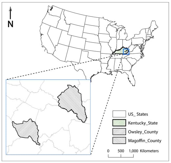
Figure 1.
Index maps showing the location of Kentucky and, within Kentucky, the locations of Magoffin and Owsley Counties.
3. Methodology
3.1. Methodological Framework
The methodology consists of two main steps: data preprocessing and model training and validation (Figure 2). In the data preprocessing step, we initially generated the training database by combining mapped landslides as positive samples and sampled four non-landslide acquisition scenarios (i.e., negative samples) from the PISA-m calculation results to evaluate the effect of negative samples on the training results. PISA-m is a physically based program that assesses slope stability by utilizing the first-order second-moment (FOSM) method based on the infinite slope assumption [,]. We provide a mathematical introduction of PISA-m in Section 3.3. For the selection of geomorphological variables as model features, we employed the Pearson correlation coefficient to assess the multicollinearity of the initially proposed variables. Ten model feature inputs, including elevation, slope, plan curvature, profile curvature, relief, distance to river, geological texture, percentage of clay, distance to road, and annual rainfall, were selected and categorized using the Jenks natural break partitioning method.
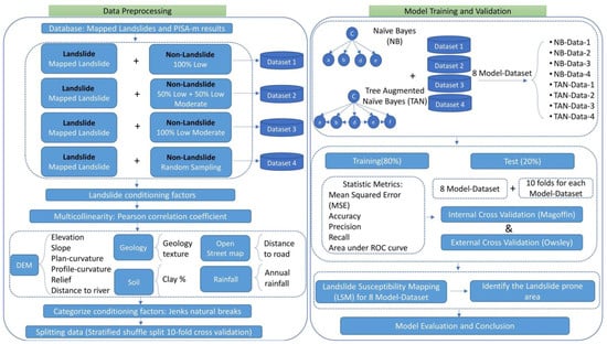
Figure 2.
Methodological flow chart of the study.
In the model training and validation step (Figure 2), we used two Bayesian network structures, namely, Naïve Bayes and Tree-augmented Naïve Bayes, to train the model based on four curated data scenarios as described in the data preprocessing step. In the assessment of model performance, we performed both internal validations based on historical landslide data in Magoffin County and external validation based on an independent inventory dataset in Owsley County. We assessed model performance using five selected statistical metrics: mean squared error (MSE), accuracy, precision, recall, and area under the receiver operating characteristic (ROC) curve. We generated LSM based on predictions from different model–data combinations and provided conclusions and discussions based on the results of model evaluation.
3.2. Landslide Mapping and Initiation Points
Landslide extents were primarily mapped by visual analysis of a multidirectional hillshade derived from a 1.5 m lidar DEM. Secondary maps, such as those showing slope, roughness, curvature, plan curvature, contour, and traditional hillshade, along with aerial photography, were employed to assist in recognizing landslide features and confirming the outlining of the extent of the deposits. The GIS polygons we digitized captured landslide extents including headscarps, flanks, toe slopes, and hummocky topography. In order to consistently capture each landslide, the polygons included headscarps, flanks, and toe slopes. For instance, the upper limit of a landslide polygon followed the slide’s crest, slightly exceeding the vertical displacement of the headscarp. While the size and shapes of smaller to moderate-sized landslides could suggest landslide types, we did not determine their age or possible behavior. Considering that over 1000 landslides were identified, conducting additional investigations that incorporate factors such as age, landslide behavior, and runout potential would be time-consuming.
We used a confidence rating system developed by the Oregon Department of Geology and Mineral Industries to interpret landslide occurrence based on the clarity of features visible in remote sensing data. A total of 1054 landslides were initially mapped in Magoffin County; this data is publicly available at https://kgs.uky.edu/kgsmap/helpfiles/landslide_help.shtm (accessed on 3 May 2023). Of these, 1.3% were deemed low confidence (≤10), 44.2% as moderate confidence (11–29), and 54.4% as high confidence (≥30). The selected landslides mean area is c. 6397 m2, with most of the landslides covering less than 25,000 m2. We removed 64 entries related to small slope slides (area ≤ 3000 m2), leaving us with 990 mapped landslides for this study.
We used PISA-m, a physically based landslide slope stability program, to assist in the identification of the initiation point (Figure 3), from which the terrain attributes were extracted for the model training. The results from PISA-m typically show that slopes have higher susceptibility values near the bottoms and then alternate between lower values and higher values as the elevation increases and the slope angle fluctuates. Landslide deposits generally did not fall into the higher probabilities of failure, which is demonstrated by the fact that the mean susceptibility by PISA-m characterization for all mapped landslide deposits is 0.05. This is because PISA-m does not attempt to discern failed slopes, which are generally less steep. On slides where steep headscarps remain, a higher probability is assigned; however, some existing slide extents are often classified as low susceptibility. In these cases, we selected the initiation points considering additional slope, roughness, curvature, and plan curvature conditions.
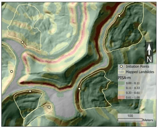
Figure 3.
Six mapped landslides and selected initiation points. Contours are PISA-m classified areas of landslide susceptibility, overlaying the hillshade of Magoffin County, Kentucky.
3.3. PISA-m Classification
PISA-m is a physically based program that assesses slope stability by utilizing the first-order second-moment (FOSM) method based on the infinite slope assumption [,]. The program uses the constitutive relationship, described by Equation (1), to calculate the factor of safety for a forested infinite slope against sliding []:
where is cohesive strength from tree roots (kPa), is cohesive strength of soil (kPa), is uniform surcharge due to vegetation (kPa), is unit weight of moist soil above phreatic surface (N/m3), is unite weight of saturated soil below phreatic surface (N/m3), is unit weight of water (9.810 N/m3), D is thickness of soil above slip surface (m), is relative height of phreatic surface above slip surface (dimensionless), is slope angle (degrees), and is angle of internal friction (degrees).
The PISA-m program requires three geospatial ASCII files that specify soil units, land cover, and digital elevation models (DEMs), along with a parameter file defining geotechnical parameters, as input. DEM, forest, and soil/geology data were generated separately for PISA-m preparation. To identify geotechnical parameters, we obtained the results of geotechnical investigations conducted by the Kentucky Transportation Cabinet and the Kentucky Geological Survey. A total of 121 geotechnical reports were collected from 1970 to 2019 for Magoffin County. As a probabilistic approach, PISA-m calculates the reliability index or probability of failure of the factor of safety being less than 1 (P[FS 1]) for the evaluation of landslide susceptibility. We used Jenks natural break method, which minimizes within-group variance and maximizes between-group variance to produce distinct clusters, to classify PISA-m results into four classes: low (0–13.5%), low-moderate (13.5–32.4%), moderate-high (32.4–58.8%), and high (58.8–100%). The PISA-m susceptibility map and its probability density function are shown in Figure 4.
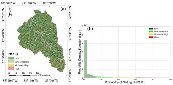
Figure 4.
(a) Magoffin PISA-m susceptibility map; (b) probability density function (pdf) of probability of sliding.
One of the objectives of the present study is to investigate the impact of negative samples on the landslide susceptibility model training. To evaluate this, we sampled four different non-landslide data scenarios from PISA-m classification results, including 100% sampled from low susceptibility areas (Data-1); 50% sampled from low susceptibility areas and 50% sampled from low-moderate susceptibility areas (Data-2); 100% sampled from low-moderate susceptibility area (Data-3); and random sampling from all susceptibility classes (Data-4). These negative samples were combined with mapped landside initiation points, as described in Section 3.2, to form the database for model training and validation (Figure 5).
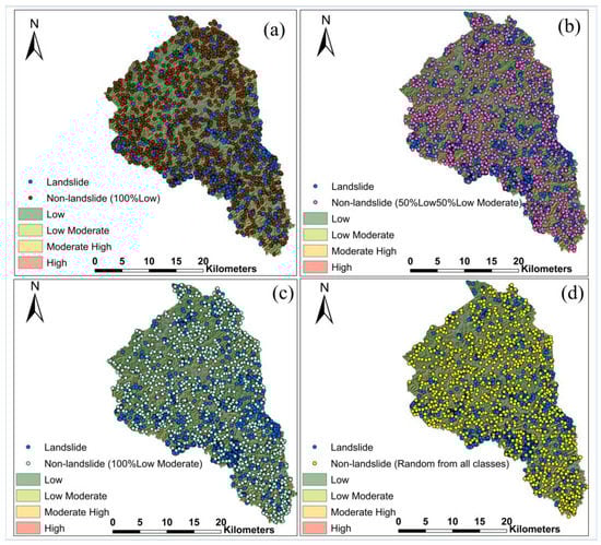
Figure 5.
Landslide inventory dataset combined with different negative sample scenarios for Magoffin County: (a) Data-1; (b) Data-2; (c) Data-3; (d) Data-4.
3.4. Geomorphic Variables
In Van Westen et al., (2008) [], the authors provided an overview of environmental factors and their relevance for landslide susceptibility and hazard assessment across various scales of analysis. At the regional scale, the topographic, geologic, hydrological, and land-use variables were generally considered highly applicable for landslide susceptibility assessment. Taking these review results into consideration, along with feature importance analyses from several previous studies [,,,], we initially considered 11 variables as inputs for the landslide susceptibility model, including elevation, slope, relief, curvature, profile curvature, plan curvature, annual rainfall, distance to river, distance to road, bedrock geology, and percentage of clay in unit soil profile. The 1.5 m resolution DEM, which was derived from airborne lidar dataset available at the KyFromAbove website (https://kyfromabove.ky.gov/, accessed on 3 May 2023), was used as the elevation factor and to derive six additional factors, including slope, curvature, plan curvature, profile curvature, relief, and distance to river. Annual rainfall data were collected from Climatic Research Unit (CRU) TS version 4.06, while distance to road data were obtained using the OpenStreetmap add-on in ArcGIS Pro. The geology data was collected from Kentucky Geological Map Service (https://kgs.uky.edu/kygeode/geomap/, accessed on 3 May 2023), and percentage of clay in unit soil profile was obtained from (https://kygeonet.ky.gov/kysoils/, accessed on 3 May 2023). The variables and their corresponding categorizations using Jenks natural break method are presented in Figure 6. It is important to note that not all geo-morphological variables have an equal impact on the model performance, and some variables, such as curvature, plan curvature, and profile curvature, are correlated with each other. Consequently, we performed multicollinearity analysis using Pearson correlation coefficient to assess correlation among independent variables and the potential overfitting problems. We did not conduct the conventional feature selection analysis by mutual information, information gain methods, etc., as the feature dimension is relatively small in this study. Moreover, structure learning in Bayesian network analysis implicitly considers the dependencies among features by searching for a maximum weighted spanning tree that maximizes the likelihood of the training data. Further details of feature analysis are presented in the Results (Section 4.1).
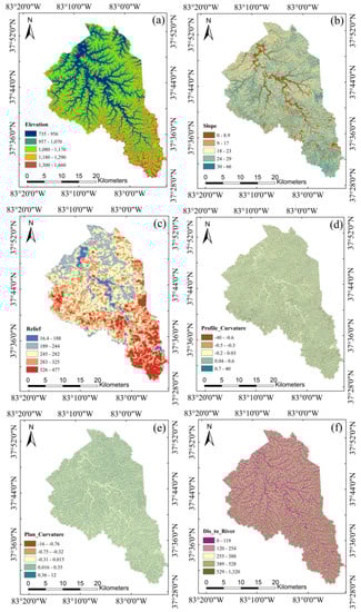
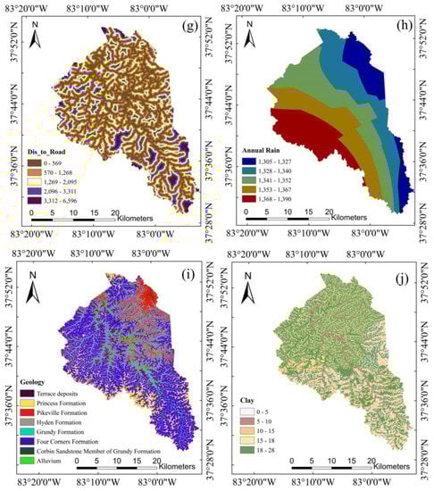
Figure 6.
The geomorphic variables used in model training: (a) elevation, (b) slope, (c) relief, (d) profile curvature, (e) plan curvature, (f) distance to river, (g) distance to road, (h) annual rainfall, (i) geology, and (j) percentage of clay in unit soil profile.
3.5. Bayesian Network Models
A Bayesian network (BN), also known as a belief network, is a graphical model that represents a probabilistic relationship between a set of random variables . It consists of a directed acyclic graph (DAG) in which every node in a Bayesian network represents a random variable . The edges in the network represent the probabilistic dependencies between the random variables, indicating that the child node is conditionally dependent on the parent node(s) . The conditional dependencies between the random variables are specified using conditional probability tables (CPTs), which specify the probability of each possible value of the child node given the values of its parent node(s) . The CPTs are used to calculate the joint probability distribution over all of the random variables in the network, which can be used to make predictions or to perform inferences about the model output(s). By explicitly modeling the dependencies among variables, Bayesian networks can provide a better understanding of the underlying causal relationships and the uncertainty associated with the model predictions. This makes them a powerful tool for natural hazard research and risk management.
We used two Bayesian network classifiers, Naïve Bayes (NB) and Tree Augmented Naïve (TAN), to produce the LSM based on the database as described in Figure 1. The construction of Bayesian networks typically involves two stages: structure learning and parameter learning. For the NB structure, no structure learning is required as it assumes all nodes are independent of each other and have landslide occurrence as their parent node. For the TAN structure, we used a score-based method based on Bayesian Dirichlet equivalent uniform (BDeu) []. The BDeu score computes the goodness-of-fit of a given network structure by considering the likelihood of the data given the network structure and the chosen prior distribution. It prefers network structures that provide a good trade-off between the complexity of the network (i.e., the number of edges or dependencies) and its ability to fit the data [].
For the parameter learning that evaluates the values of the CPTs, we used Bayesian estimation, which updates the prior knowledge using observed data within the Bayesian statistical framework. The key idea behind Bayesian estimation is to combine prior beliefs about the parameters with the observed data to obtain a posterior distribution, which represents the updated beliefs about the parameters after taking the data into account. In this study, we used Dirichlet prior, which is the conjugate prior for multinomial likelihood, resulting in Dirichlet posteriors for mathematical convenience. The details of parameter learning are presented in the following section, Section 3.5.1.
3.5.1. Naïve Bayes
Naïve Bayes (NB) is a simple and efficient classifier that assumes that the input variables are conditionally independent given the class label. This means that no structure learning is required and that the presence or absence of one input variable does not affect the probability of the other input variables. Despite its simple model structure and the independent assumption, NB can still perform well in many landslide susceptibility modeling studies [,,].
The NB structure yields a unique joint probability [], as shown in Equation (2):
where C is the class node, and are attribute nodes.
To compute the CPTs, we need to determine the prior and likelihood function to perform Bayesian estimation. In this study, we used Dirichlet prior, which is the conjugate prior for multinomial likelihood. The prior and the likelihood function is shown in Equations (3) and (5), respectively. The posterior distribution can be calculated as Equation (6) []:
where , are the Dirichlet hyperparameters. A higher shows a Dirichlet distribution with higher density. Dirichlet hyperparameters are often called pseudo-counts, which can be understood as the number of occurrences of different outcomes before counting from the present experiment. In multinomial sampling, the observed variable is discrete, having possible states, and . is a distribution describing the mean prediction of our prior and can be defined as Equation (4):
where
where . denotes the number of samples in which the variable adopts the value and the parent nodes adopt the configuration state . is the sum of for the whole dataset. is BDeu score where is the user-determined equivalent sample size, is the number of possible values and is the number of configuration. is the sum of for the whole dataset.
3.5.2. Tree Augmented Naïve Bayes
The Tree Augmented Naive Bayes (TAN) model is a variant of the Naive Bayes algorithm, which allows for dependencies between input variables []. Each variable node can have at most one parent node from other variables with the exception of the class variable (Equation (7)):
For TAN structure, the search algorithm is based on Tree search and, in this study, uses mutual information score to find the most significant dependency between each pair of attributes. The conditional mutual information is defined as follows [] (Equation (8)):
Assuming a set of as four attribute nodes, if corresponds to maximum mutual information, the arc between and is added to the structure of TAN. This process is followed by finding the second most significant dependence where is the parent and is the child of . At this stage, the parent and child nodes are restricted in a way that and . The process is iterated until all the variables have one dependence relationship between any variables. At the end, a root node is selected, and all the edges go outward from it, and the class node is going toward all the attribute variables as the parent of all nodes.
3.6. Internal and External Validation
For model validation, each of the four datasets generated in this study, as illustrated in Figure 1, was split into training (80%) and testing (20%) subsets. K-fold cross-validation was used to partition each dataset into K folds, with K-1 folds used to create estimators and the remaining fold used for testing []. The model used a different fold as the test set each time and was tested K times to reduce the possibility of overfitting and sampling bias.
We used five evaluation metrics, including mean squared error (MSE), accuracy, precision, recall, and area under the curve (AUC), to assess the performance of each model–data combination as shown in Figure 1. Equations (9)–(13) present the expressions for each metric. In Equations (10)–(12), function terms are derived from conventional confusion matrix and are as follows: TP represents true positives, TN represents true negatives, FP represents false positives, and FN represents false negatives. The AUC value is associated with the receiver operating characteristic (ROC) curve, where the latter is a graphical representation that plots the true positive (sensitivity) against the false positive (1-specificity) for different threshold values. An AUC score of 1 indicates perfect classification, while a score of 0.5 represents random performance. According to [], the AUC value can be classified into four levels: poor (0.5–0.6), moderate (0.6–0.7), good (0.7–0.8), and excellent (0.9–1).
4. Results and Analysis
4.1. Multicollinearity Analysis
In this study, we performed the multicollinearity analysis by computing the Pearson correlation coefficient on the initial 11 variables and their correlations to the landslide occurrence to acquire an understanding of the correlation nature of the variables. The results shown in Figure 7 present the correlation matrices for four datasets, with matrix values ranging from −1 to +1 where zero indicates no correlation and ±1 indicates perfect positive or negative linear correlation. The plot shows that the variables curvature, plan curvature, and profile curvature are highly correlated with each other in all data scenarios, which is as anticipated due to their close physical definitions. Moreover, the curvature has the lowest correlation with landslide occurrence among all variables; therefore. we removed it in the model training process.
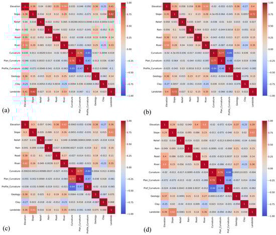
Figure 7.
Correlation matrices for multicollinearity analysis of datasets: (a) Data-1; (b) Data-2; (c) Data-3; (d) Data-4.
4.2. Model Performance and Validation
We used five different validation metrics (i.e., AUC, ACC, precision, recall, and MSE) to evaluate the model performance for eight different model–dataset combinations (i.e., NB-Data-1, NB-Data-2, NB-Data-3, NB-Data-4, TAN-Data-1, TAN-Data-2, TAN-Data-3, and TAN-Data-4). A ten-fold cross validation as introduced in Section 3.6 was conducted to assess the model performance based on the selected metrics. Table 1 summarizes the range and median values of the validation metrics computed from the cross-validations results, demonstrating acceptable model performance for all model–dataset scenarios, with metric ranges of 0.79 < Accuracy < 0.94, 0.78 < Precision < 0.97, 0.82 < Recall < 0.94, 0.06 < MSE < 0.20, and 0.88 < AUC < 0.98.

Table 1.
Range and median values of validation metrics computed from cross-validation results of eight different model–dataset combinations.
Figure 8 presents the violin plots for five evaluation metrics, which includes the box plots, along with rotated kernel density plots on each side. The probability distributions indicate that the trained TAN-Data-1 model exhibited the best performance, as evidenced by the lower MSE and higher AUC, accuracy, recall, and precision values. For the Bayesian network structure comparison, TAN outperformed the NB structure in both means and variations for all data scenarios. Conversely, when the model structure is the same, dataset-1, which sampled all non-landslides from PISA-m low susceptibility areas, demonstrated the best modeling result for internal validation. With the inclusion of more negative samples extracted from PISA-m low-moderate susceptibility areas, corresponding to data scenarios moved from Data-1 to Data-3, the training outcomes declined in all metric evaluations, for both TAN or NB model structures. This suggests that high contrast training data would result in better landslide classification for internal validation. However, we further examined this conclusion by conducting external validation using an independent landslide repository for Owsley counties, Kentucky, as introduced in Section 4.4.
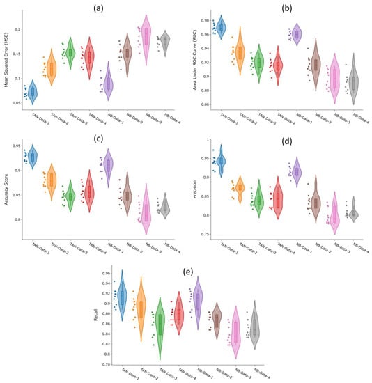
Figure 8.
Results of validation metrics for eight model–dataset combinations: (a) mean squared error (MSE); (b) area under ROC curve (AUC); (c) accuracy score; (d) precision; (e) recall.
Figure 8 presents the mean ROC curves, calculated by averaging the ten-fold cross-validation results, based on eight different model–dataset combinations. Each of the ROC curves was constructed using false positive rates versus true positive rates at ten different thresholds (i.e., 10%, 20%, 30%, 40%, 50%, 60%, 70%, 80%, 90%, and 100%). According to Figure 8, both models and datasets influence the classification outcomes. The use of Data-1, which sampled negative samples exclusively from PISA-m low susceptibility areas, produced the best model performance for both the TAN or NB structures. This corroborates our hypothesis that landslide classification is greatly sensitive to the selection of negative samples. From Figure 9, we also observed that the TAN model consistently outperformed the NB model when the dataset was the same, and model performance declined from Data-1 to Data-4. This trend aligns with the violin plots of validation metrics presented in Figure 8. The modeling differences between TAN and NB models are consistent with findings from Lee, S. et al. [] and Pham, B. et al. [], which show that considering feature dependencies by the Bayesian network assumption can lead to better model performance compared to the independent assumption among model features by the NB structure.
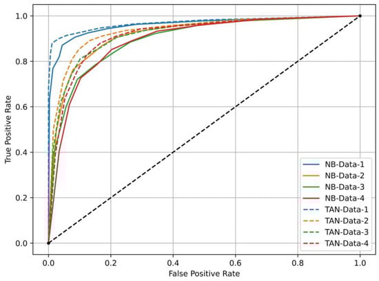
Figure 9.
Mean of ROC curves for eight model–dataset combinations.
4.3. Landslide Susceptibility Maps
After internal validation, we produced the LSM based on each trained model’s predictions. Figure 10 presents the LSM generated by four trained models—NB-data-1, NB-data-3, TAN-data-1, and TAN-data-3—along with local zoomed-in susceptibility maps showing the estimations of landslide occurrence as exposed to different topographic conditions, including mountain tops, steep slopes, valley bottoms, etc. The results show that, for flat mountain tops, predictions based on the NB model classify the majority of areas as high susceptibility (Figure 10a,e), whereas the same areas are mainly classified as moderate by the TAN model classification. This suggests that elevation may play an important role in NB model predictions, regardless of slope conditions. Figure 10b,f,j,n show landforms characterized by steep ridgetops and concave slopes. In NB classifications (Figure 10b,f), steep slopes just below ridgetops are characterized as high or moderate-high susceptibility, while flank, toe, and flow channels are mostly characterized as low susceptibility. On the other hand, the TAN models characterize a significant number of concave slopes as moderate-high or high susceptibility areas (Figure 10j,n), particularly slopes below main headscarps. Figure 10d,h,l,p show areas with steep ridgetops and planar or convex slopes. According to BN model predictions, ridgetops and steep slopes close to mountain ridges and heads of catchments are related to high landslide susceptibility. This classification aligns well with the results reported by He et al., (2019) [] and Lee et al., (2020) [], in which the NB models identified many ridgetops and the corresponding flanks as high susceptibility areas. The TAN model classification is similar to that of the NB model in this case as indicated by the comparison between Figure 10d,l, except that the ridgetop is largely excluded by the TAN model classifications. This fits the empirical understanding of landslide occurrences starting below the crown of the slope. The overall results comparison suggests that the predictions by the TAN models produced more realistic LSMs compared to those of NB models, with the former highlighting the high susceptibility areas associated with varying slopes and hummocky topography.
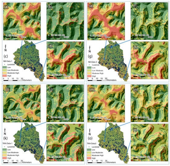
Figure 10.
Magoffin landslide susceptibility mapping (LSM) based on predictions from four trained models. (c) shows the LSM based on trained model NB-Data-1, with (a,b,d) as zoomed-in views of local areas. (g) shows the LSM based on trained model NB-Data-3, with (e,f,h) as zoomed-in views of local areas. (k) shows the LSM based on trained model TAN-Data-1, with (i,j,l) as zoomed-in views of local areas. (o) shows the LSM based on trained model TAN-Data-3, with (m,n,p) as zoomed-in views of local areas.
Figure 11 presents the probability density function (PDF) calculated from eight susceptibility maps, along with the classification obtained by averaging Jenks natural break partitioning for each produced LSM. All PDFs follow a decaying trend with high probability associated with low susceptibility areas and low probability associated with high susceptibility areas, suggesting that most districts in Magoffin County are not considered as landslide-prone areas. Figure 11 also demonstrates the impact of training datasets on overall susceptibility classification—more areas are classified as moderate susceptibility rather than low susceptibility if there is less restriction on negative samples being selected from the low susceptibility class in PISA-m classification, as reflected from dataset scenarios moved from Data-1 to Data-3. Note that the positive samples derived from the landslide inventory are the same for all training models; therefore, the results indicate that less contrastive training datasets yield less polarized predictions.
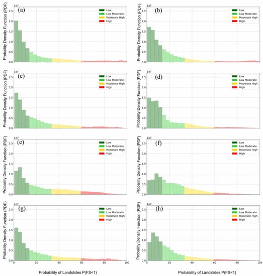
Figure 11.
Probability density function of Magoffin LSM calculated from (a) NB-Data-1; (b) TAN-Data-1; (c) NB-Data-2; (d) TAN-Data-2; (e) NB-Data-3; (f) TAN-Data-3; (g) NB-Data-4; (h) TAN-Data-4.
Figure 12 presents the summarized probability of each susceptibility class for the eight trained models. The results corroborate the similar trend shown in Figure 11, indicating that more contrastive positive–negative training samples produce more polarized predictions, as evidenced by the data comparison from Data-1 to Data-3 for both NB and TAN cases. Figure 12 also demonstrates the impacts of model structures, with the NB model estimating more areas as moderate-high or high susceptibility compared to the TAN model. This may be due to elevation being considered as a significant influencing factor in NB model predictions, as illustrated in the susceptibility maps (Figure 10).
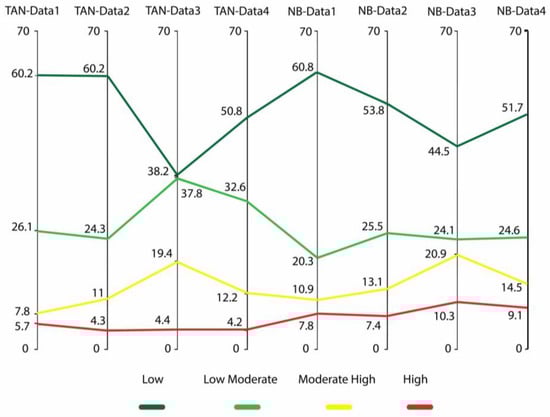
Figure 12.
Summarized probability of each susceptibility class from eight trained models.
4.4. External Validation
To evaluate the reliability of the eight trained models mentioned earlier, we conducted further external validation using an independent landslide inventory covering Owsley County, which does not share a common border but is situated in close vicinity to Magoffin County (Figure 1). The original inventory contains 1344 mapped landslides, from which we adopted 636 landslides (Figure 13). Each adopted landslide has at least an overall moderate confidence ranking (≥11), as introduced in Section 3.2. The same types of geomorphic variables (elevation, slope, relief, profile curvature, plan curvature, distance to river, distance to road, annual rainfall, geology texture, and percentage of clay) were pre-processed and used as model input for the eight trained models for the Owsley case study (Figure 14).
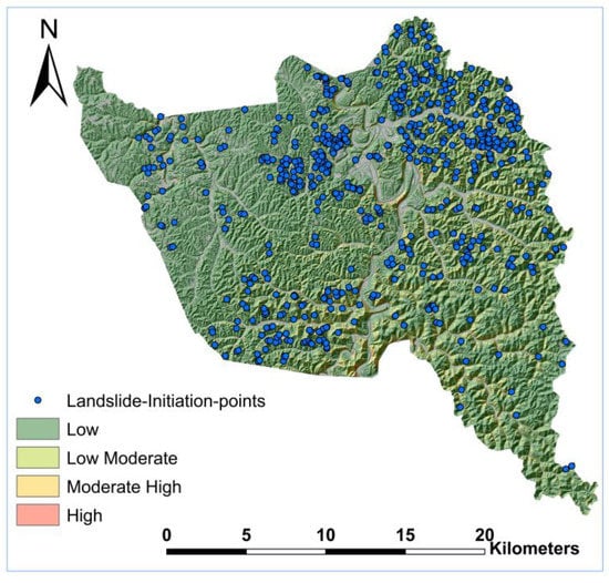
Figure 13.
Landslide inventory dataset of Owsley County, KY, USA.
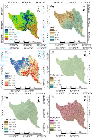
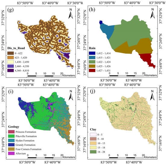
Figure 14.
The geomorphic variables used in model training for Owsley County, KY, USA: (a) elevation, (b) slope, (c) relief, (d) profile curvature, (e) plan curvature, (f) distance to river, (g) distance to road, (h) annual rainfall, (i) geology, and (j) percentage of clay in unit soil profile.
After calculating LSMs, we determined the classification thresholds by averaging the eight computed thresholds from participating LSMs. The resulting susceptibility classes are as follows: low (0–14.8%), low-moderate (14.8–30.4%), moderate-high (30.4–50.7%), and high (50.7–100%). Figure 15 presents the classification outcomes for mapped landslide initiation points and the total area of Owsley County, based on each model’s predictions. The model comparison again corroborated that the TAN model always outperformed the NB model when the training dataset was the same, as shown by the high percentage of landslide points characterized in moderate-high and high classes by the former. It was observed that NB models produced an approximately uniform estimation across four landslide susceptibility classes for landslide initiation points (between 20% and 30%), which was demonstrated as not practically useful for LSM analysis. In contrast, TAN models generally produced satisfying results, with combined moderate-high and high susceptibility equal to 71.22%, 95.91%, 86.01%, and 74.06% for models TAN-Data-1 to TAN-Data-4.
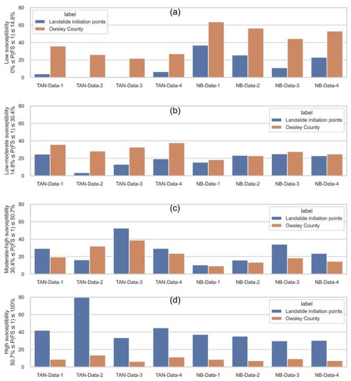
Figure 15.
Susceptibility classifications for Owsley County computed using eight trained models: (a) percentages of mapped landslide initiation points and total county area classified as low susceptibility; (b) percentages of mapped landslide initiation points and total county area classified as low-moderate susceptibility; (c) percentages of mapped landslide initiation points and total county area classified as moderate-high susceptibility; (d) percentages of mapped landslide initiation points and total county area classified as high susceptibility.
However, the former most effective model, TAN-Data-1, yielded the least effective modeling results in external validation, while the TAN-Data-2 model, which comprised its negative training sample with a mixture of 50% low and 50% low-moderate susceptibilities from PISA-m predictions, represented the top-performing model in current analysis. This implies that the conventional method of sampling non-landslide areas exclusively from very flat surfaces or low susceptibility areas can result in overfitting models, which performed no better than a random selection of negative samples (TAN-Data-4), as shown in the present study. The results of the present study suggest that employing a prior physical model estimation and selecting a balanced negative sample to represent non-landslide scenarios can improve the robustness of model performance and should be considered for future similar studies.
Figure 16 shows the local susceptibility maps generated by TAN-Data-1 and TAN-Data-2 models. By comparing the subplots shown in Figure 16a,b, it is evident that TAN-Data-1 produced more binary predictions of either high or low susceptibilities. In contrast, TAN-Data-2 generated more gradual results following the strike of the slope. This trend is also visible when comparing the subplots shown in Figure 16c,d, where TAN-Data-1 classifies flat mountain tops as high susceptibility areas, while TAN-Data-2 assigns them moderate-high susceptibility, with a more gradual transition between high and low susceptibility zones. These observations indicate that the more balanced samples used for training the TAN-Data-2 model result in a more nuanced and realistic representation of landslide susceptibility observed across Owsley County.
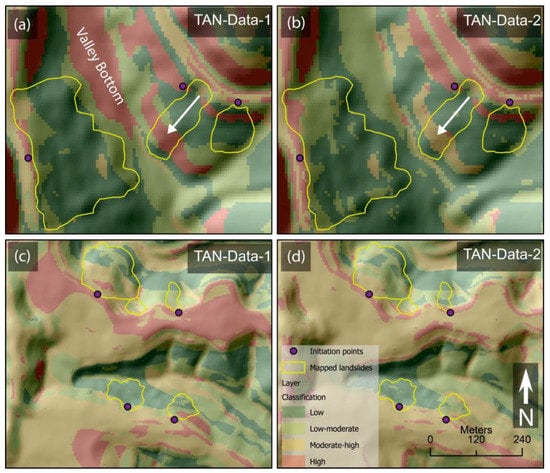
Figure 16.
Local susceptibility classifications for Owsley County computed using TAN-Data1 and TAN-Data2 models. Subplots (a,b) represent the same area with different susceptibility characterizations based on predictions from the TAN-Data-1 and TAN-Data-2 models, respectively. Similarly, subplots (c,d) display another comparative analysis of the same area, showing susceptibility predictions from the TAN-Data-1 and TAN-Data-2 models.
5. Discussion
The application of machine learning coupled with remote sensing data in landslide susceptibility assessment has rapidly proliferated over the past two decades. Remote sensing data, which are typically high-resolution and cover wide areas, can provide valuable geospatial information that is crucial for identifying and delineating landslide-prone areas. Meanwhile, the machine learning technique can effectively manage the large volume and diverse datasets, incorporating topological, hydrological, geological, vegetation, and even human factors into modeling considerations. This integration would be challenging in a constitutive model, in which describing and maintaining such relationships can be difficult.
Given this increasing trend of machine-learning-based landslide characterization, however, there are some long-standing issues, which directly impact the reliability and robustness of previously proposed models and remain unresolved or inadequately considered in the literature, including uncertainties associated with training samples, model structures, and mode validations. To the best of the authors’ knowledge, few studies have considered the impact of negative samples in natural hazard model training. This could be due to the complexity of defining non-hazard scenarios during the sampling process. As discussed in the previous sections, a “non-landslide” point can only be accurate temporarily, as potential landslides are subject to constant change and development. Relying on the assumption that “the past and the present are keys to the future” [] in landslide characterization may prove insufficient for both positive and negative aspects of training samples. Furthermore, the practice of selecting negative samples from very flat surfaces or low susceptibility areas, as adopted in some previous research [,], has been shown to be ineffective in external validation in the present study.
The impact of model types and structures is also relevant in landslide characterization. Various machine learning methods, including logistic regression, support vector machines, random forest, and artificial neural networks, among others, have been applied in related research. In this study, we used BN models and assessed two model structures to estimate landslide susceptibility. As a probabilistic graphical approach, BN models offer several advantages that are crucial for predicting natural hazards like landslides. First, BN models provide a visual representation of the relationships between variables, making it easier for decision-makers and stakeholders to understand the underlying assumptions and dependencies in the model. This transparency can improve communication and trust in predictions, which is not available in black-box models. Additionally, BN models can represent and quantify uncertainties in the relationships between variables, which is particularly useful in predicting natural hazards like landslides, where complete knowledge of the underlying processes is often lacking. This essential data-mining process is valuable for identifying the most critical factors influencing landslide risk and supporting targeted interventions or data collection efforts, which are of future research interest for the authors.
In regard to the model comparison between the NB and TAN structures, the results consistently showed that the latter produced better predictions in terms of evaluation metrics including MSE, accuracy, precision, recall, and AUC. This finding aligns well with several previous studies that compared NB and Bayesian network modeling outcomes using different landslide inventory datasets [,,]. We noticed that the susceptibility predictions generated by NB models tend to be polarized, as illustrated by the classification of most areas into either very high or very low landslide susceptibility categories in LSM. This classification pattern, also reported by Lee et al. [], may be due to the assumption of independence between model features inherent to the NB model structure, which in turn could reduce the flexibility of model predictions leading to dramatic but potentially less realistic susceptibility classifications.
Lastly, we also emphasized the importance of robustness validation for machine learning models in natural hazard characterizations, such as landslides. We observed considerable differences between the most effective models in internal validation and those that performed unsatisfactorily in external validation, which demonstrated the potential overfitting problem. This issue has been long-standing, yet it has not been seriously considered in many previous studies. However, we do not intend to provide an optimal solution to this problem in the present study as that would require a comprehensive database that includes more morphological illustrations of landslides under various scenarios and a rigorous grid search for balanced training datasets. We recognize that the present study may raise more questions than solutions, but this can ultimately lead to improved landslide hazard characterization and more effective risk mitigation strategies.
6. Conclusions
In this study, we assessed the impact of negative samples and Bayesian network structures on landslide susceptibility characterization using two landslide inventories from Kentucky, USA. By utilizing a physically based susceptibility evaluation, we generated four non-landslide data scenarios that were combined with mapped landslides to produce landslide susceptibility maps using two Bayesian network model structures.
In model training and internal validation, we used five different validation metrics (i.e., AUC, ACC, precision, recall, and MSE) to evaluate the model performance for eight different model–dataset combinations (i.e., NB-Data-1, NB-Data-2, NB-Data-3, NB-Data-4, TAN-Data-1, TAN-Data-2, TAN-Data-3, and TAN-Data-4). For the Bayesian network structure comparison, TAN outperformed the NB structure in both means and variations of validation metrics for all data scenarios. Conversely, when the model structure remained consistent, dataset-1, which selected all non-landslides from PISA-m low susceptibility areas, yielded the best results for internal validation. Furthermore, we produced the LSMs based on each trained model’s predictions. For NB classifications, the steep slopes located just below the ridgetops were largely classified as high or moderate-high susceptibility, while the flanks, toes, and flow channels were mainly characterized as low susceptibility. In contrast, the TAN model classified a significant number of concave slopes as moderate-high or high susceptibility areas, which fits the empirical understanding of landslide occurrence typically initiating below the slope’s crown.
To evaluate the reliability of the eight trained models, we conducted further external validation using an independent landslide inventory covering Owsley County, Kentucky, USA. The model comparison again suggested that the TAN model always outperformed the NB model when the training dataset was the same, as indicated by the high percentage of landslide points characterized in moderate-high and high classes by the former. However, the previously leading model TAN-Data-1 yielded the least effective modeling results in external validation, while the TAN-Data-2 model, which comprised its negative training sample with a mixture of 50% low and 50% low-moderate susceptibilities from PISA-m predictions, represented the top-performing model in external validation. This implies that the conventional method of sampling non-landslide areas exclusively from very flat surfaces or low susceptibility areas can result in overfitting models, which performed no better than the random selection of negative samples (TAN-Data-4), as shown in the present work.
Our results suggest employing a prior physical model estimation and selecting a balanced negative sample to represent non-landslide scenarios and enhance the model’s robustness. Building on these insights, our future research aims to explore more effective probabilistic modeling structures and optimize the integration of physical knowledge into landslide susceptibility modeling.
Author Contributions
Conceptualization, Y.Z. and W.C.H.; methodology, Y.Z. and S.K.; validation, S.K. and Y.Z.; formal analysis, S.K.; investigation, S.K., Y.Z., and M.M.C.; resources, Y.Z.; data curation, Y.Z., M.M.C., and H.J.K.; writing—original draft preparation, S.K.; writing—review and editing, Y.Z. and M.M.C.; visualization, S.K. and Y.Z.; supervision, Y.Z. and W.C.H.; project administration, Y.Z.; funding acquisition, Y.Z. All authors have read and agreed to the published version of the manuscript.
Funding
This research was funded by startup funding provided by Temple University, grant number 143487-23030-02.
Data Availability Statement
The landslide inventory for Magoffin County, Kentucky, is publicly available at https://kgs.uky.edu/kgsmap/helpfiles/landslide_help.shtm (accessed on 3 May 2023). The 1.5 m resolution DEM, which was derived from an airborne lidar dataset, is available at the KyFromAbove website: https://kyfromabove.ky.gov/ (accessed on 3 May 2023). The geology data in this research was collected from the Kentucky Geological Map Service: https://kgs.uky.edu/kygeode/geomap/ (accessed on 3 May 2023). The soil data was obtained from https://kygeonet.ky.gov/kysoils/ (accessed on 3 May 2023).
Acknowledgments
We would like to thank Joseph Thomas Coe, Heyang (Harry) Yuan, and Mehdi Khanzadeh Moradllo from Temple University for their project reviews. The authors also appreciate the editorial assistance of Rachel Noble-Varney at Kentucky Geological Survey.
Conflicts of Interest
The authors declare they have no competing financial interests or personal relationships that could be conflict of interest.
References
- Farrokhnia, A.; Pirasteh, S.; Pradhan, B.; Pourkermani, M.; Arian, M. A Recent Scenario of Mass Wasting and Its Impact on the Transportation in Alborz Mountains, Iran Using Geo-Information Technology. Arab. J. Geosci. 2011, 4, 1337–1349. [Google Scholar] [CrossRef]
- Froude, M.J.; Petley, D.N. Global Fatal Landslide Occurrence from 2004 to 2016. Nat. Hazards Earth Syst. Sci. 2018, 18, 2161–2181. [Google Scholar] [CrossRef]
- Crawford, M.M. Kentucky Geological Survey Landslide Inventory: From Design to Application. In Kentucky Geological Survey Information Circular; University of Kentucky: Lexington, KY, USA, 2014; Volume 21. [Google Scholar] [CrossRef]
- Crawford, M.M.; Bryson, L.S. Assessment of Active Landslides Using Field Electrical Measurements. Eng. Geol. 2017, 233, 146–159. [Google Scholar] [CrossRef]
- Guzzetti, F.; Reichenbach, P.; Cardinali, M.; Galli, M.; Ardizzone, F. Probabilistic Landslide Hazard Assessment at the Basin Scale. Geomorphology 2005, 72, 272–299. [Google Scholar] [CrossRef]
- Crawford, M.M.; Dortch, J.M.; Koch, H.J.; Killen, A.A.; Zhu, J.; Zhu, Y.; Bryson, L.S.; Haneberg, W.C. Using Landslide-Inventory Mapping for a Combined Bagged-Trees and Logistic-Regression Approach to Determining Landslide Susceptibility in Eastern Kentucky, USA. Q. J. Eng. Geol. Hydrogeol. 2021, 54, qjegh2020-177. [Google Scholar] [CrossRef]
- Bui, D.T.; Tuan, T.A.; Klempe, H.; Pradhan, B.; Revhaug, I. Spatial Prediction Models for Shallow Landslide Hazards: A Comparative Assessment of the Efficacy of Support Vector Machines, Artificial Neural Networks, Kernel Logistic Regression, and Logistic Model Tree. Landslides 2016, 13, 361–378. [Google Scholar]
- Anagnostopoulos, G.G.; Fatichi, S.; Burlando, P. An Advanced Process-Based Distributed Model for the Investigation of Rainfall-Induced Landslides: The Effect of Process Representation and Boundary Conditions. Water Resour. Res. 2015, 51, 7501–7523. [Google Scholar] [CrossRef]
- Alvioli, M.; Baum, R.L. Parallelization of the TRIGRS Model for Rainfall-Induced Landslides Using the Message Passing Interface. Environ. Model. Softw. 2016, 81, 122–135. [Google Scholar] [CrossRef]
- Van Westen, C.; Terlien, M.J.T. An Approach towards Deterministic Landslide Hazard Analysis in GIS. A Case Study from Manizales (Colombia). Earth Surf. Process. Landf. 1996, 21, 853–868. [Google Scholar] [CrossRef]
- Reichenbach, P.; Rossi, M.; Malamud, B.D.; Mihir, M.; Guzzetti, F. A Review of Statistically-Based Landslide Susceptibility Models. Earth Sci. Rev. 2018, 180, 60–91. [Google Scholar] [CrossRef]
- Merghadi, A.; Yunus, A.P.; Dou, J.; Whiteley, J.; ThaiPham, B.; Bui, D.T.; Avtar, R.; Abderrahmane, B. Machine Learning Methods for Landslide Susceptibility Studies: A Comparative Overview of Algorithm Performance. Earth Sci. Rev. 2020, 207, 103225. [Google Scholar] [CrossRef]
- Zhou, X.; Wen, H.; Li, Z.; Zhang, H.; Zhang, W. An Interpretable Model for the Susceptibility of Rainfall-Induced Shallow Landslides Based on SHAP and XGBoost. Geocarto Int. 2022, 37, 13419–23450. [Google Scholar] [CrossRef]
- Sahana, M.; Pham, B.T.; Shukla, M.; Costache, R.; Thu, D.X.; Chakrabortty, R.; Satyam, N.; Nguyen, H.D.; Van Phong, T.; Van Le, H.; et al. Rainfall Induced Landslide Susceptibility Mapping Using Novel Hybrid Soft Computing Methods Based on Multi-Layer Perceptron Neural Network Classifier. Geocarto Int. 2022, 37, 2747–2771. [Google Scholar] [CrossRef]
- Guzzetti, F.; Reichenbach, P.; Ardizzone, F.; Cardinali, M.; Galli, M. Estimating the Quality of Landslide Susceptibility Models. Geomorphology 2006, 81, 166–184. [Google Scholar] [CrossRef]
- Petschko, H.; Brenning, A.; Bell, R.; Goetz, J.; Glade, T. Assessing the Quality of Landslide Susceptibility Maps—Case Study Lower Austria. Nat. Hazards Earth Syst. Sci. 2014, 14, 95–118. [Google Scholar] [CrossRef]
- Tsangaratos, P.; Ilia, I. Comparison of a Logistic Regression and Naïve Bayes Classifier in Landslide Susceptibility Assessments: The Influence of Models Complexity and Training Dataset Size. Catena 2016, 145, 164–179. [Google Scholar] [CrossRef]
- Peng, L.; Niu, R.; Huang, B.; Wu, X.; Zhao, Y.; Ye, R. Landslide Susceptibility Mapping Based on Rough Set Theory and Support Vector Machines: A Case of the Three Gorges Area, China. Geomorphology 2014, 204, 287–301. [Google Scholar] [CrossRef]
- Kavzoglu, T.; Sahin, E.K.; Colkesen, I. Landslide Susceptibility Mapping Using GIS-Based Multi-Criteria Decision Analysis, Support Vector Machines, and Logistic Regression. Landslides 2014, 11, 425–439. [Google Scholar] [CrossRef]
- Hu, Q.; Zhou, Y.; Wang, S.; Wang, F. Machine Learning and Fractal Theory Models for Landslide Susceptibility Mapping: Case Study from the Jinsha River Basin. Geomorphology 2020, 351, 106975. [Google Scholar] [CrossRef]
- Huang, F.; Cao, Z.; Jiang, S.-H.; Zhou, C.; Huang, J.; Guo, Z. Landslide Susceptibility Prediction Based on a Semi-Supervised Multiple-Layer Perceptron Model. Landslides 2020, 17, 2919–2930. [Google Scholar] [CrossRef]
- Dou, J.; Yunus, A.P.; Bui, D.T.; Merghadi, A.; Sahana, M.; Zhu, Z.; Chen, C.-W.; Khosravi, K.; Yang, Y.; Pham, B.T. Assessment of Advanced Random Forest and Decision Tree Algorithms for Modeling Rainfall-Induced Landslide Susceptibility in the Izu-Oshima Volcanic Island, Japan. Sci. Total Environ. 2019, 662, 332–346. [Google Scholar] [CrossRef] [PubMed]
- McDowell, R.C. The Geology of Kentucky: A Text to Accompany the Geologic Map of Kentucky; Professional Paper 1151-H; US Geological Survey: Reston, VA, USA, 1986. [Google Scholar]
- Chapella, H.; Haneberg, W.; Crawford, M.; Shakoor, A. Landslide Inventory and Susceptibility Models, Prestonsburg 7.5-Min Quadrangle, Kentucky, USA. In Proceedings of the IAEG/AEG Annual Meeting Proceedings, San Francisco, CA, USA, 17–21 September 2018; Springer: Cham, Switzerland, 2019; Volume 1, pp. 217–226. [Google Scholar]
- Crawford, M.M.; Dortch, J.M.; Koch, H.J.; Zhu, Y.; Haneberg, W.C.; Wang, Z.; Bryson, L.S. Landslide Risk Assessment in Eastern Kentucky, USA: Developing a Regional Scale, Limited Resource Approach. Remote Sens. 2022, 14, 6246. [Google Scholar] [CrossRef]
- Burns, W.J.; Madin, I.P. Protocol for Inventory Mapping of Landslide Deposits from Light Detection and Ranging (Lidar) Imagery; DOGAMI Special Paper; Oregon Department of Geology and Mineral Industries: Lake County, OR, USA, 2009; Volume 42. [Google Scholar]
- Haneberg, W.C. A Rational Probabilistic Method for Spatially Distributed Landslide Hazard Assessment. Environ. Eng. Geosci. 2004, 10, 27–43. [Google Scholar] [CrossRef]
- Haneberg, W.C. Deterministic and Probabilistic Approaches to Geologic Hazard Assessment. Environ. Eng. Geosci. 2000, 6, 209–226. [Google Scholar] [CrossRef]
- Hammond, C. Level I Stability Analysis (LISA) Documentation for Version 2.0; US Department of Agriculture, Forest Service, Intermountain Research Station: Ogden, UT, USA, 1992; Volume 285. [Google Scholar]
- Van Westen, C.J.; Castellanos, E.; Kuriakose, S.L. Spatial Data for Landslide Susceptibility, Hazard, and Vulnerability Assessment: An Overview. Eng. Geol. 2008, 102, 112–131. [Google Scholar] [CrossRef]
- Tien Bui, D.; Pradhan, B.; Lofman, O.; Revhaug, I. Landslide Susceptibility Assessment in Vietnam Using Support Vector Machines, Decision Tree, and Naive Bayes Models. Math. Probl. Eng. 2012, 2012, 974638. [Google Scholar] [CrossRef]
- Pham, B.T.; Pradhan, B.; Bui, D.T.; Prakash, I.; Dholakia, M.B. A Comparative Study of Different Machine Learning Methods for Landslide Susceptibility Assessment: A Case Study of Uttarakhand Area (India). Environ. Model. Softw. 2016, 84, 240–250. [Google Scholar] [CrossRef]
- Pham, B.T.; Tien Bui, D.; Indra, P.; Dholakia, M. Landslide Susceptibility Assessment at a Part of Uttarakhand Himalaya, India Using GIS–Based Statistical Approach of Frequency Ratio Method. Int. J. Eng. Res. Technol. 2015, 4, 338–344. [Google Scholar]
- Koller, D.; Friedman, N. Probabilistic Graphical Models: Principles and Techniques; MIT Press: Cambridge, MA, USA, 2009. [Google Scholar]
- Cooper, G.F.; Herskovits, E. A Bayesian Method for the Induction of Probabilistic Networks from Data. Mach. Learn. 1992, 9, 309–347. [Google Scholar] [CrossRef]
- Nhu, V.H.; Shirzadi, A.; Shahabi, H.; Singh, S.K.; Al-Ansari, N.; Clague, J.J.; Jaafari, A.; Chen, W.; Miraki, S.; Dou, J.; et al. Shallow Landslide Susceptibility Mapping: A Comparison between Logistic Model Tree, Logistic Regression, Naïve Bayes Tree, Artificial Neural Network, and Support Vector Machine Algorithms. Int. J. Environ. Res. Public Health 2020, 17, 2749. [Google Scholar] [CrossRef]
- Sajadi, P.; Sang, Y.F.; Gholamnia, M.; Bonafoni, S.; Mukherjee, S. Evaluation of the Landslide Susceptibility and Its Spatial Difference in the Whole Qinghai-Tibetan Plateau Region by Five Learning Algorithms. Geosci. Lett. 2022, 9, 9. [Google Scholar] [CrossRef]
- Dey, L.; Chakraborty, S.; Biswas, A.; Bose, B.; Tiwari, S. Sentiment Analysis of Review Datasets Using Naive Bayes and K-NN Classifier. Int. J. Inf. Eng. Electron. Bus. 2016, 8, 54–62. [Google Scholar] [CrossRef]
- Heckerman, D. A Tutorial on Learning with Bayesian Networks; Springer: Dordrecht, The Netherlands, 1998; Volume 89. [Google Scholar]
- Friedman, N.; Geiger, D.; Goldszmidt, M. Bayesian Network Classifiers. Mach. Learn. 1997, 29, 131–163. [Google Scholar] [CrossRef]
- Picard, R.R.; Cook, R.D. Cross-Validation of Regression Models. J. Am. Stat. Assoc. 1984, 79, 575–583. [Google Scholar] [CrossRef]
- Wu, Y.; Ke, Y.; Chen, Z.; Liang, S.; Zhao, H.; Hong, H. Application of Alternating Decision Tree with AdaBoost and Bagging Ensembles for Landslide Susceptibility Mapping. Catena 2020, 187, 104396. [Google Scholar] [CrossRef]
- Lee, S.; Lee, M.-J.; Jung, H.-S.; Lee, S. Landslide Susceptibility Mapping Using Naïve Bayes and Bayesian Network Models in Umyeonsan, Korea. Geocarto Int. 2020, 35, 1665–1679. [Google Scholar] [CrossRef]
- He, Q.; Shahabi, H.; Shirzadi, A.; Li, S.; Chen, W.; Wang, N.; Chai, H.; Bian, H.; Ma, J.; Chen, Y.; et al. Landslide Spatial Modelling Using Novel Bivariate Statistical Based Naïve Bayes, RBF Classifier, and RBF Network Machine Learning Algorithms. Sci. Total Environ. 2019, 663, 1–15. [Google Scholar] [CrossRef]
- Orme, J. Social Work: Gender, Care and Justice. Br. J. Soc. Work. 2002, 32, 799–814. [Google Scholar] [CrossRef]
Disclaimer/Publisher’s Note: The statements, opinions and data contained in all publications are solely those of the individual author(s) and contributor(s) and not of MDPI and/or the editor(s). MDPI and/or the editor(s) disclaim responsibility for any injury to people or property resulting from any ideas, methods, instructions or products referred to in the content. |
© 2023 by the authors. Licensee MDPI, Basel, Switzerland. This article is an open access article distributed under the terms and conditions of the Creative Commons Attribution (CC BY) license (https://creativecommons.org/licenses/by/4.0/).