
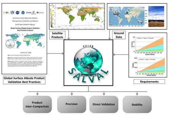
Surface ALbedo VALidation (SALVAL) Platform: Towards CEOS LPV Validation Stage 4—Application to Three Global Albedo Climate Data Records

 ,
, 

 ,
, 
Abstract
1. Introduction
2. Methods and Datasets: The SALVAL Tool
2.1. Validation Methodology
2.2. Satellite Datasets
2.2.1. NASA MCD43A3 C6.1
2.2.2. C3S Multi-Sensor V2
2.2.3. BNU GLASS V4
2.2.4. Summary and Quality Flags
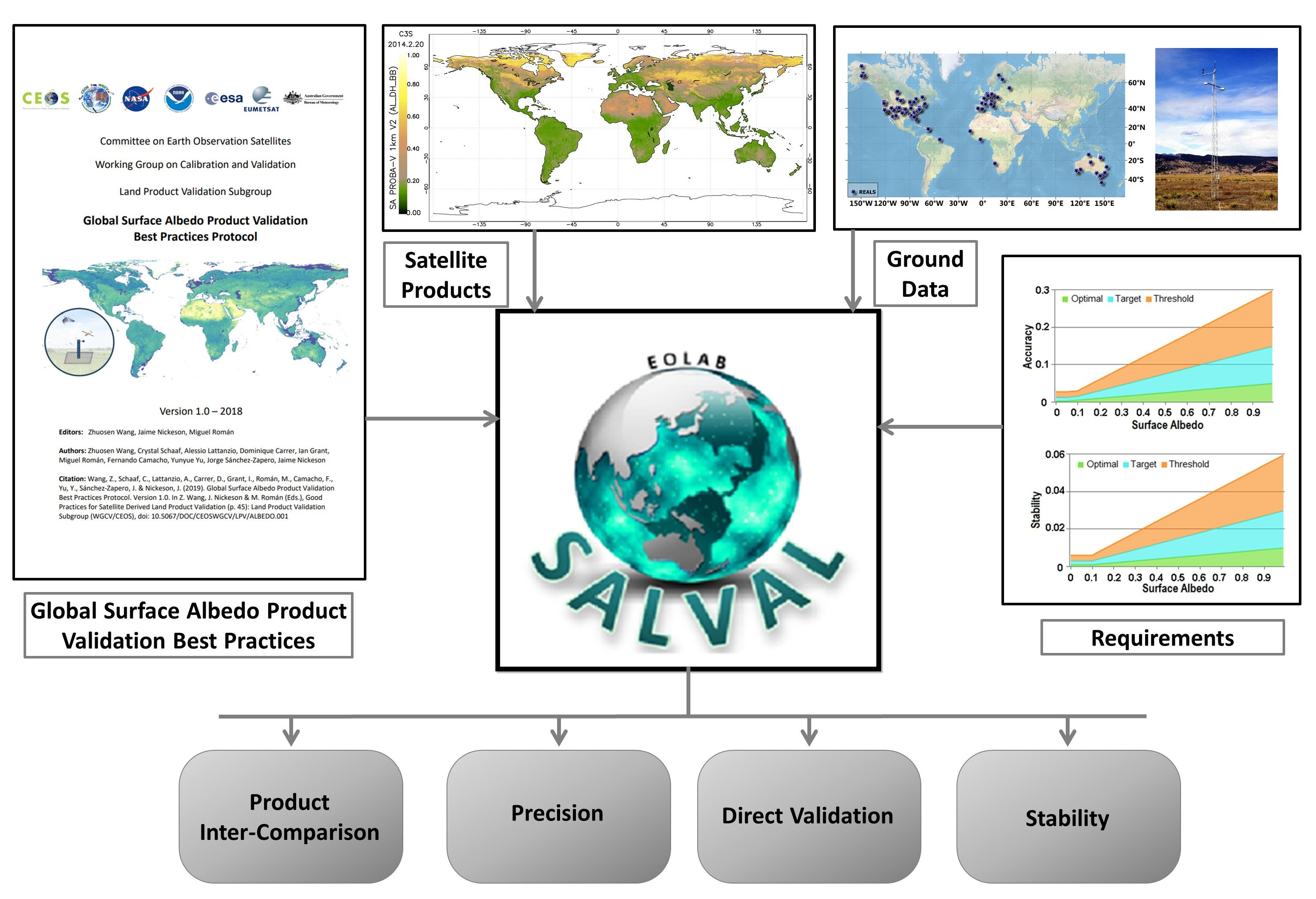
2.3. Representativeness-Evaluated ALbedo Stations (REALS) Dataset
2.4. SALVAL Functionalities and Configuration
3. Results
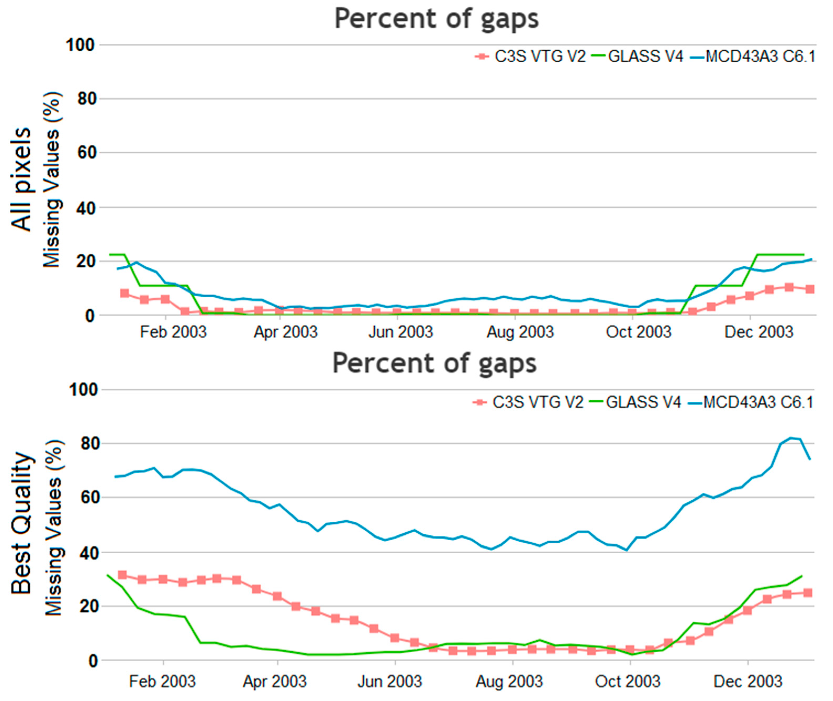
3.1. Product Completeness
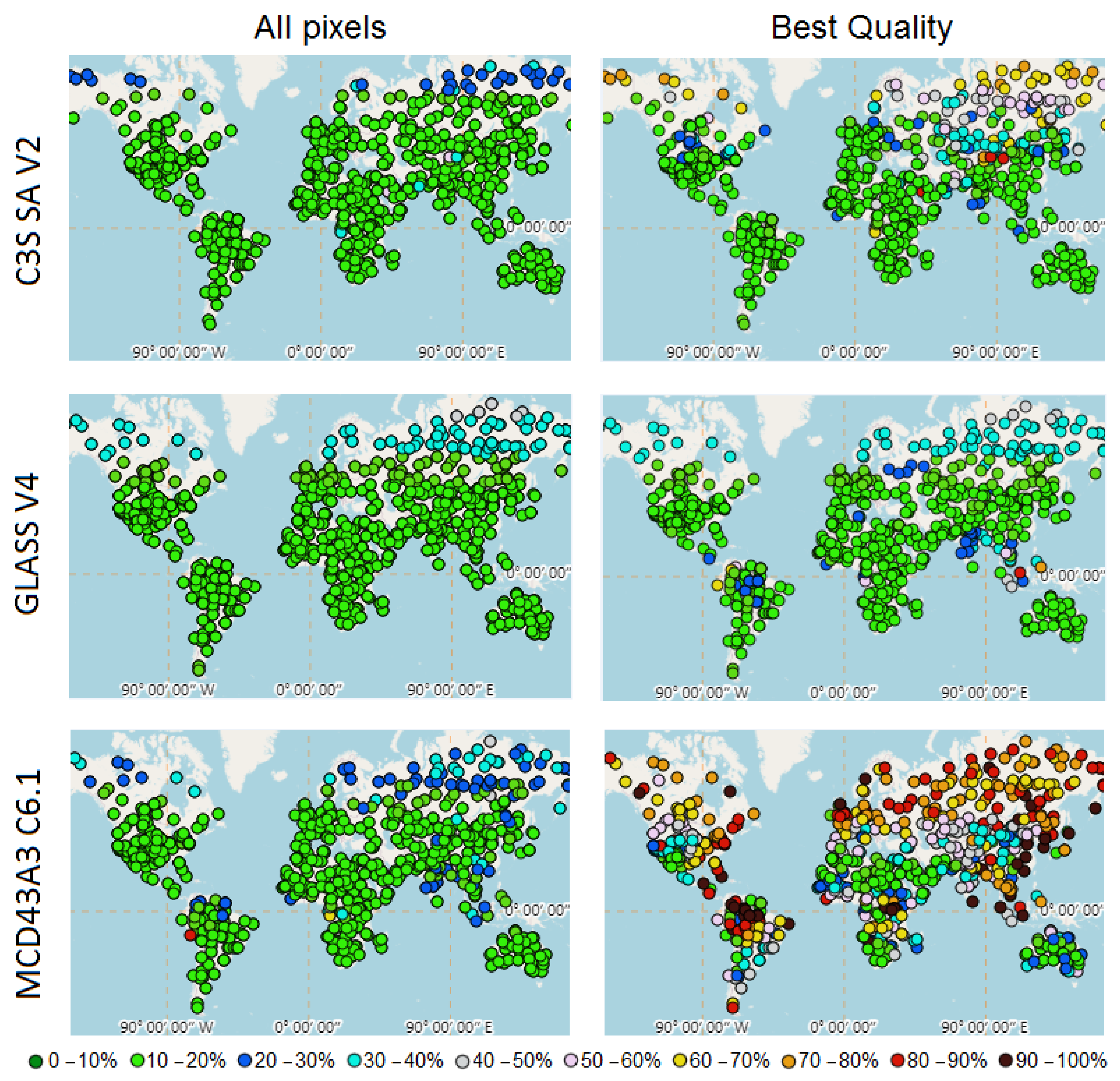
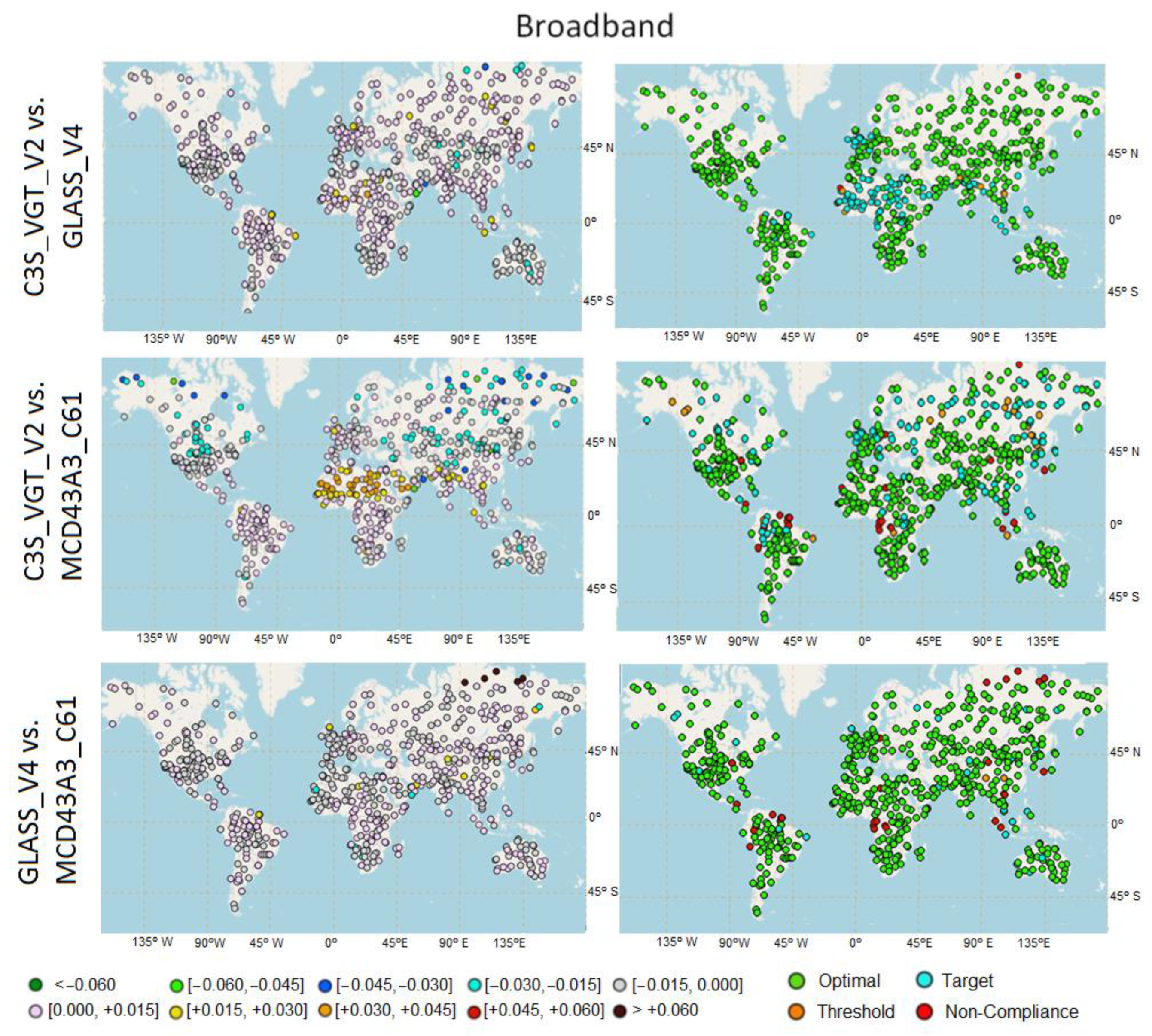
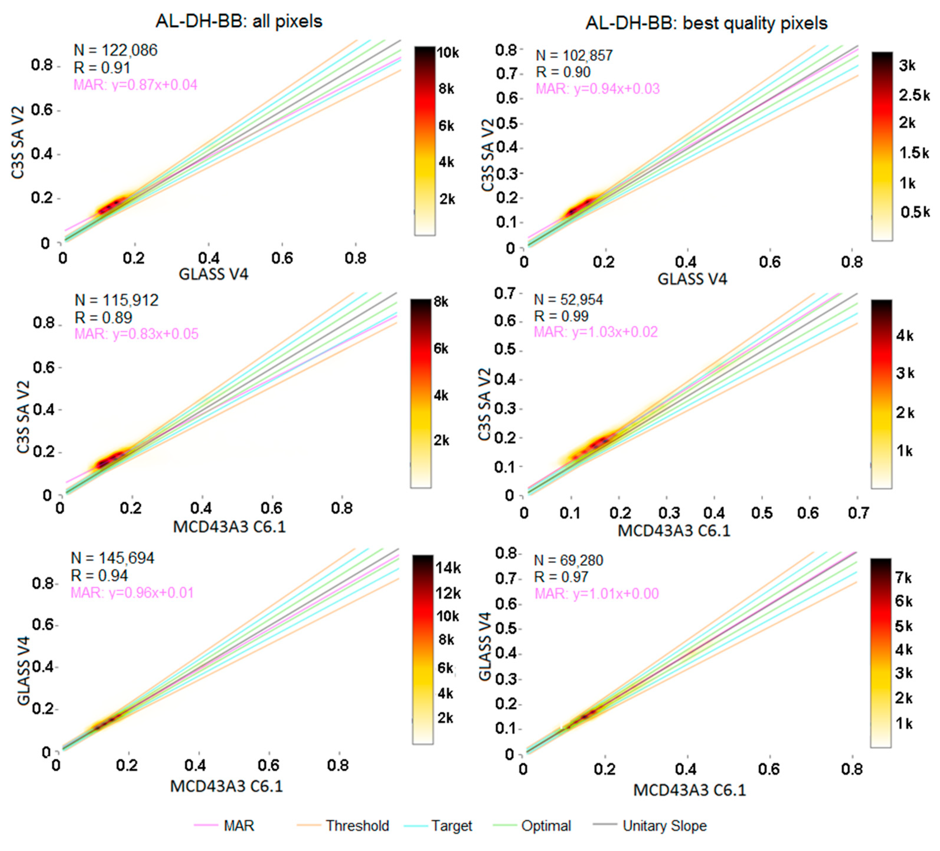
3.2. Spatial Consistency
3.3. Temporal Consistency
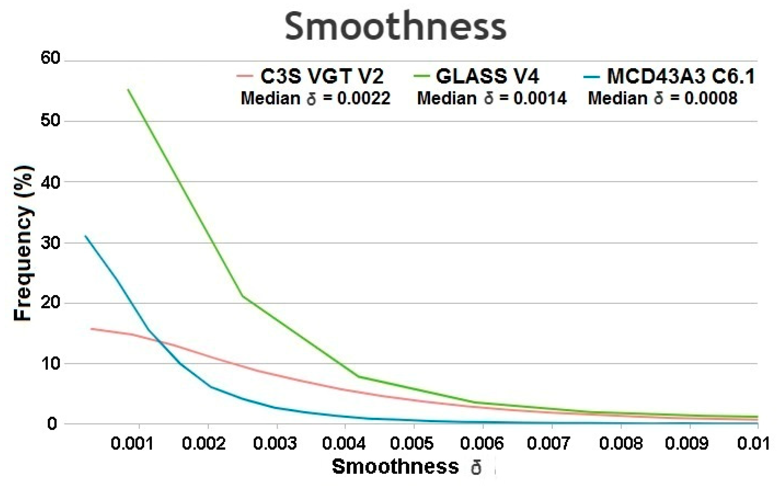
3.4. Intra-Annual Precision
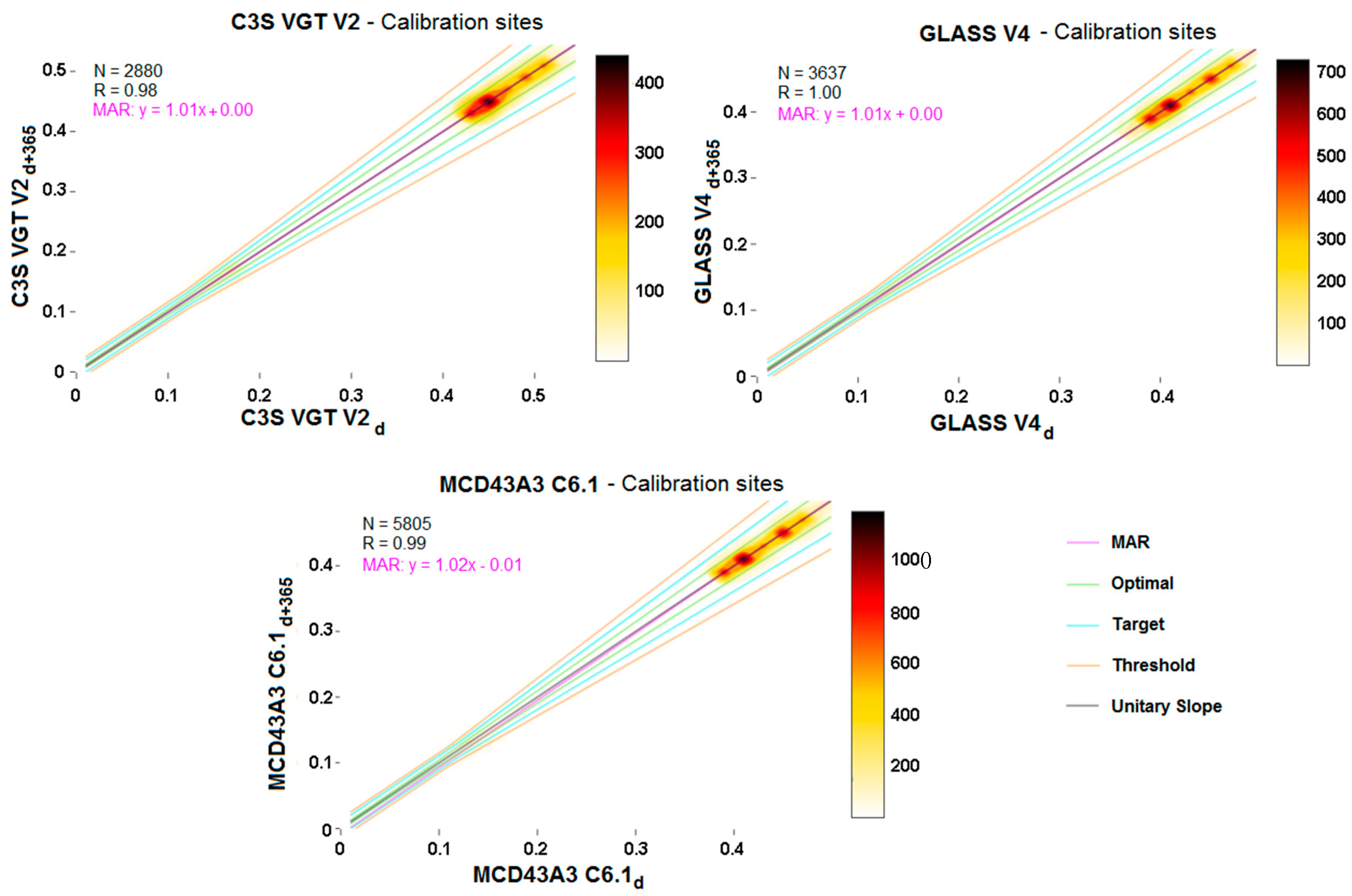
3.5. Inter-Annual Precision
3.6. Overall Spatio-Temporal Consistency
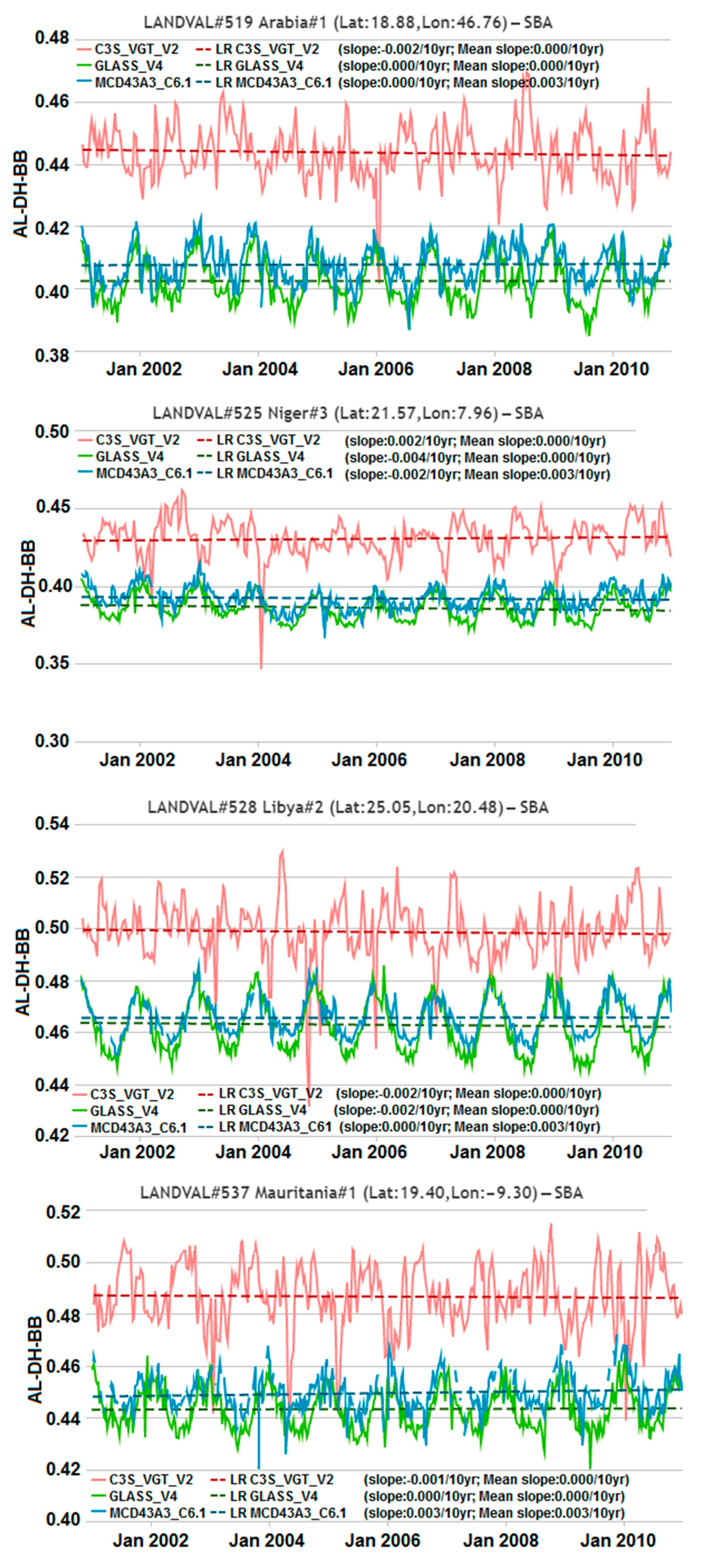
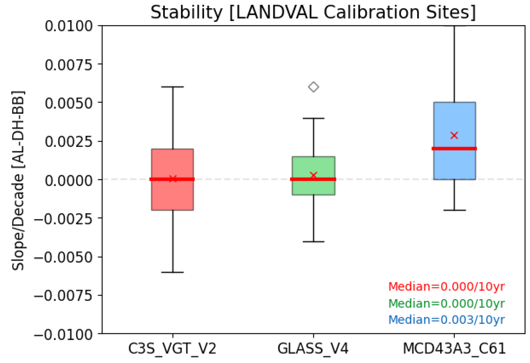
3.7. Stability
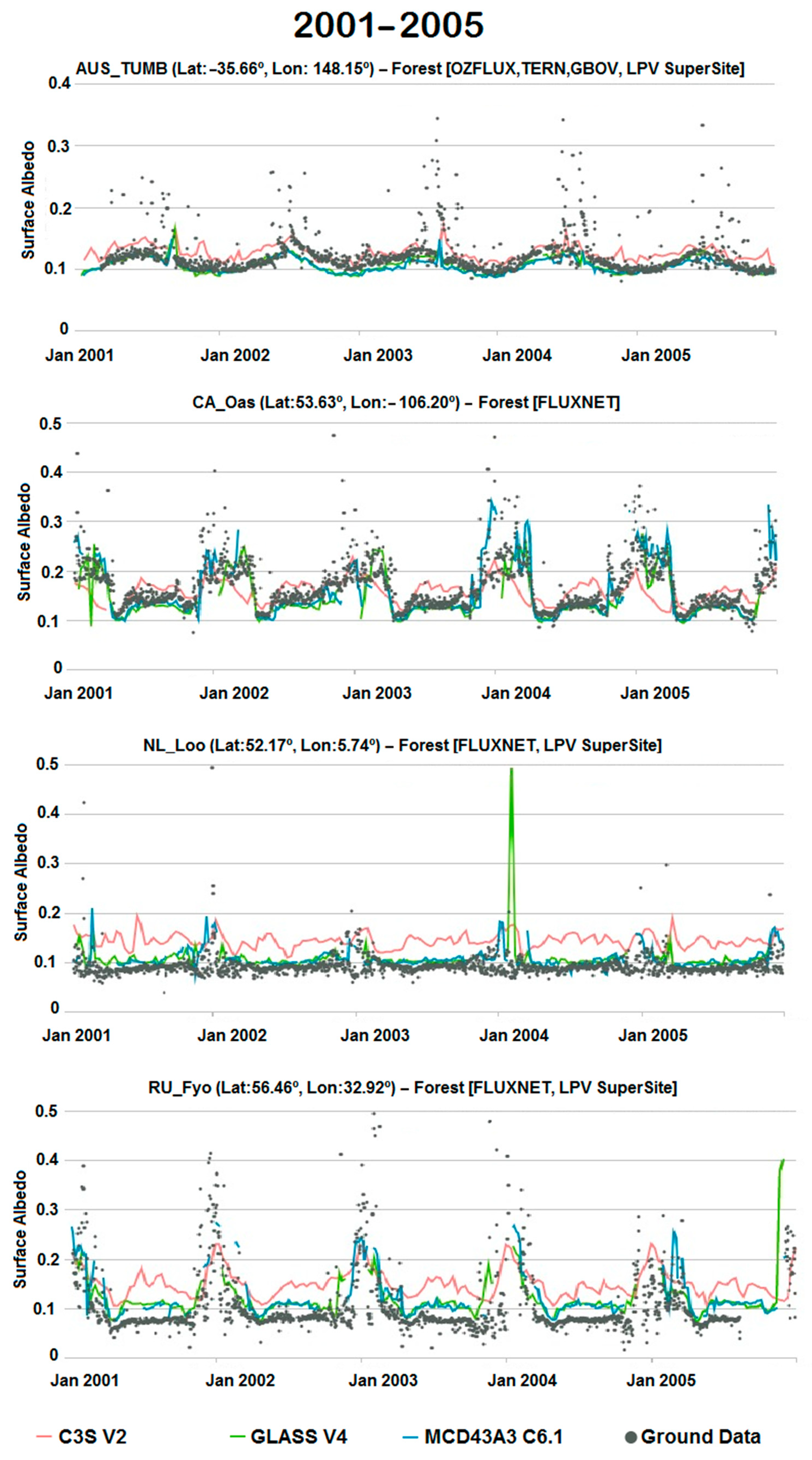
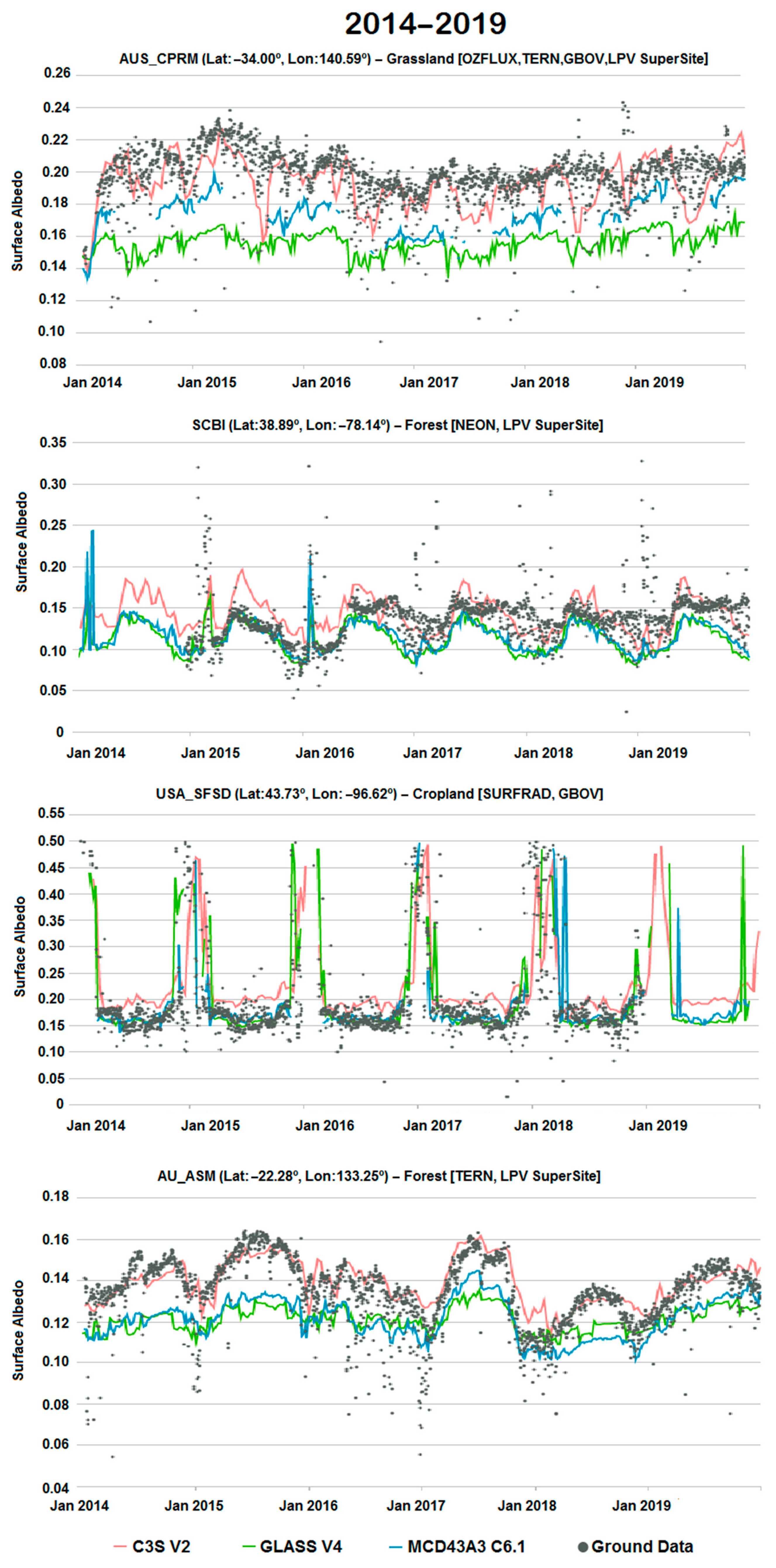
3.8. Direct Validation
4. Discussion
5. Conclusions
Author Contributions
Funding
Data Availability Statement
Acknowledgments
Conflicts of Interest
Abbreviations
| ADEOS | ADvanced Earth Observing Satellite |
| AL-BH | Bi-Hemispherical ALbedos |
| AL-DH | Directional-Hemispherical Albedos |
| APU | Accuracy, Precision and Uncertainty |
| AVHRR | Advanced Very High Resolution Radiometer |
| B | Mean Bias |
| BHR | Bi-Hemispherical Reflectance |
| BNU | Beijing Normal University’s |
| BRDF | Bidirectional Reflectance Distribution Function |
| BSA | Black-Sky Albedo |
| BSRN | Baseline Surface Radiation Network |
| C3S | Copernicus Climate Change Service |
| Cal/Val | Calibration/Validation |
| CDR | Climate Data Record |
| CDS | Climate Data Store |
| CEOS | Committee on Earth Observation Satellites |
| CGLS | Copernicus Global Land Service |
| CMG | Climate Modelling Grid |
| CUL | CULtivated |
| DBF | Deciduous Broadleaved Forest |
| DHR | Directional-Hemispherical Reflectance |
| EBF | Evergreen Broadleaved Forest |
| ECV | Essential Climate Variable |
| EFDC | European Fluxes Database Cluster |
| EOLAB | Earth Observation LABoratory |
| EPS | EUMETSAT Polar System |
| ESA | European Space Agency |
| FLUXNET | FLUXes NETwork |
| GBOV | Ground-Based Observations for Validation |
| GCOS | Global Climate Observing System |
| GLASS | Global LAnd Surface Satellites |
| GSD | Ground Sampling Distance |
| HER | HERbaceous |
| ICOS | Integrated Carbon Observation System |
| JCGM | Joint Committee for Guides in Metrology |
| LANDVAL | LAND VALidation network |
| LPDAAC | Land Processes Distributed Active Archive Center |
| LPV | Land Product Validation subgroup |
| MAD | Median Absolute Deviation |
| MAR | Major Axis Regression |
| MCD43 | TERRA + AQUA MODIS BRDF/Albedo/NBAR Product |
| MD | Median Deviation |
| MetOp | Polar-orbiting Meteorological satellites |
| MODIS | MODerate resolution Imaging Spectroradiometer |
| MSG | Meteosat Second Generation |
| N | Number of samples |
| NASA | National Aeronautics and Space Agency |
| NEON | National Science Foundation’s National Ecological Observatory Network |
| NIR | Near-Infrared |
| NLF | Needle-Leaf Forest |
| NOAA | National Oceanic and Atmospheric Administration |
| OF | Other Forests |
| Probability Density Function | |
| POLDER | POLarization and Directionality of the Earth’s Reflectances |
| PROBA-V | Project for Onboard Autonomy satellite, the V standing for vegetation |
| R | Correlation coefficient |
| RCV | Relative Coefficient of Variation |
| REALS | Representativeness-Evaluated ALbedo Stations |
| RMSD | Root Mean Square Deviation |
| RSE | Scale REequirement index |
| RST | Relative STrength of the spatial correlation |
| RSV | Relative proportion of Structural Variation |
| RTM | Radiative Transfer Model |
| SA | Surface Albedo |
| SALVAL | Surface ALbedo VALidation tool |
| RAW | First order score |
| SBA | Sparse and Bare Areas |
| SEVIRI | Spinning Enhanced Visible and Infrared Imager |
| SHR | SHRublands |
| SMAC | Simplified Method for Atmospheric Correction |
| SPOT | Satellites for the Observation of the Earth |
| ST | STandard score |
| STD | Standard deviation |
| STF | Statistics-based Temporal Filtering |
| SURFRAD | SURFace RADiation budget network |
| SW | ShortWave |
| TERN | Australia’s Land Ecosystem Observatory or Terrestrial Ecosystem |
| TOA | Top-Of-Atmosphere |
| TOC | Top-Of-Canopy |
| VGT | VeGeTation sensor |
| WGCV | Working Group on Calibration and Validation |
| WMO | World Meteorological Organization |
| WSA | White-Sky Albedo |
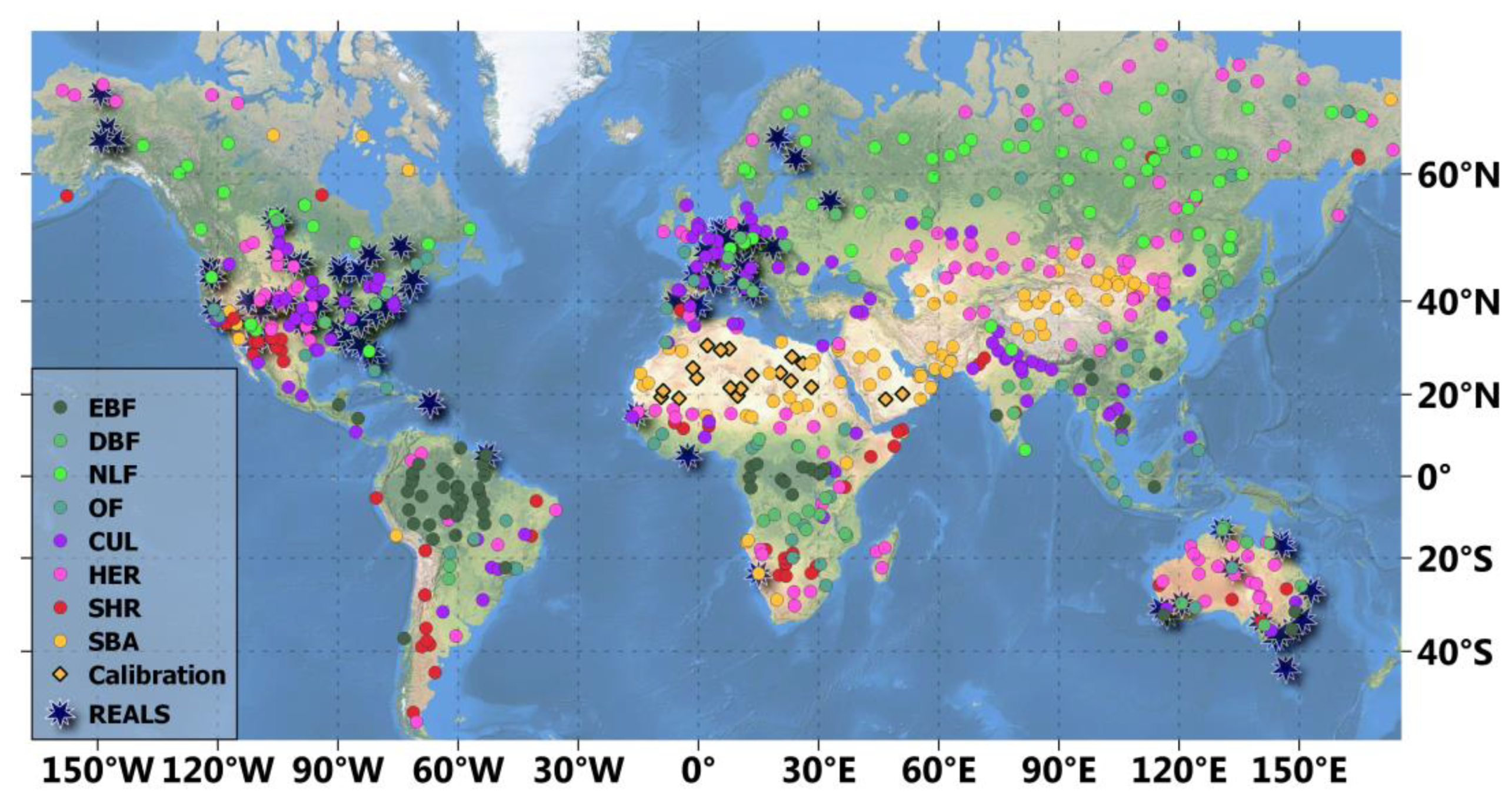
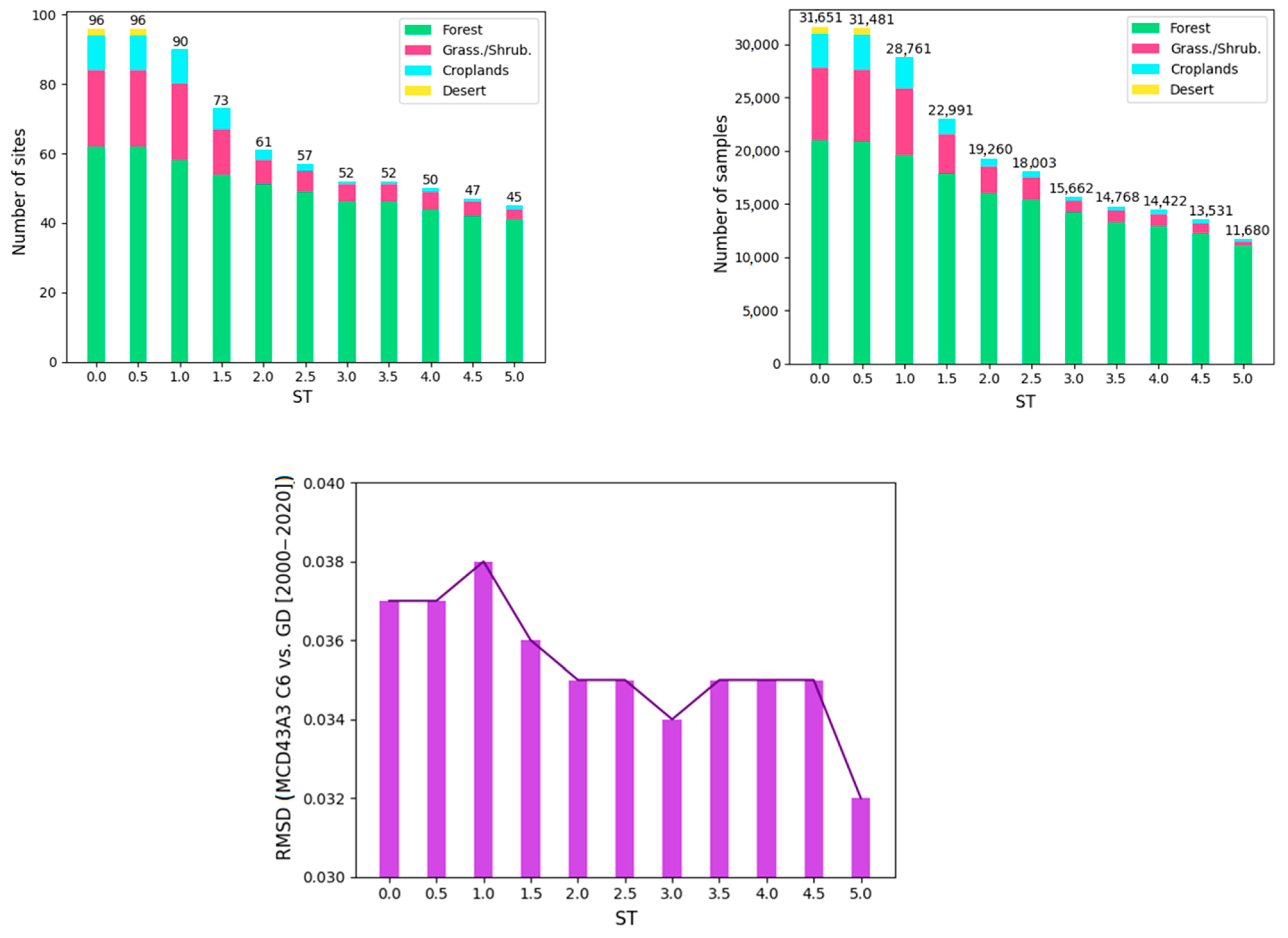
Appendix A. REALS Sites’ Characteristics and ST Scores

| ID | Code | Latitude | Longitude | Name | Network | Class | ST Leaf-Off | ST Leaf-On |
|---|---|---|---|---|---|---|---|---|
| 1 | USA_BOND | 40.05192 | −88.37309 | Bondville | SURFRAD, GBOV | Croplands | 1.52 | 1.58 |
| 2 | USA_BAOR | 40.05005 | −105.00387 | Boulder | BSRN, GBOV | Croplands | 1.29 | 2.98 |
| 3 | BEL_BRAS | 51.30761 | 4.51984 | Brasschaat | FLUXNET, GBOV(LPV SuperSite) | Forest | 19.36 | 10.42 |
| 4 | NET_CABA | 51.97100 | 4.92700 | Cabauw | BSRN, GBOV | Grass/shrub | 13.86 | 6.65 |
| 5 | AUS_CPRM | −34.00270 | 140.58771 | Calperum | OZFLUX, TERN, GBOV(LPV SuperSite) | Grass/shrub | 2.72 | 2.83 |
| 6 | USA_DRAK | 36.62418 | −116.01990 | Desert Rock | SURFRAD, GBOV | Desert | 0.96 | 0.96 |
| 7 | USA_FPEK | 48.30783 | −105.10170 | Fort Peck | SURFRAD, GBOV | Grass/shrub | 1.85 | 1.60 |
| 8 | GER_GEBE | 51.10010 | 10.91430 | Gebesee | FLUXNET, GBOV | Croplands | 1.08 | 1.22 |
| 9 | NAM_GOBA | −23.56184 | 15.04131 | Gobabeb | BSRN, GBOV(LPV SuperSite) | Desert | 0.95 | 0.87 |
| 10 | USA_GCMK | 34.25505 | −89.87360 | Goodwin Creek | SURFRAD, GBOV | Forest | 2.92 | 1.96 |
| 11 | FRA_GRIG | 48.84420 | 1.95191 | Grignon | FLUXNET, GBOV | Croplands | 1.04 | 1.05 |
| 12 | FRA_GUYA | 5.27877 | −52.92486 | Guyaflux | FLUXNET, GBOV(LPV SuperSite) | Forest | 5.47 | 5.47 |
| 13 | GER_HAIN | 51.07920 | 10.45220 | Hainich | FLUXNET, GBOV(LPV SuperSite) | Forest | 6.84 | 18.17 |
| 14 | USA_NRFT | 40.03287 | −105.54690 | Niwot Ridge Forest | FLUXNET, GBOV | Forest | 4.06 | n/a |
| 15 | ITA_RENO | 46.58690 | 11.43370 | Renon | FLUXNET, GBOV | Forest | 1.45 | 1.79 |
| 16 | USA_PSUS | 40.72012 | −77.93085 | Rock Springs | SURFRAD, GBOV | Forest | 1.04 | 2.96 |
| 17 | USA_SFSD | 43.73403 | −96.62331 | Sioux Falls SurfRad | SURFRAD, GBOV | Croplands | 1.85 | 2.11 |
| 18 | USA_SGP | 36.60575 | −97.48876 | Southern Great Plains | SURFRAD, GBOV | Croplands | 1.02 | 0.80 |
| 19 | USA_TBLN | 40.12498 | −105.23680 | Table Mountain | SURFRAD, GBOV | Desert | 2.24 (*) | 2.24 (*) |
| 20 | AUS_TUMB | −35.65652 | 148.15163 | Tumbarumba | OZFLUX, TERN, GBOV (LPV SuperSite) | Forest | 11.65 | 11.65 |
| 21 | LENO | 31.85388 | −88.16122 | Lenoir Landing | NEON | Forest | 2.33 | 4.96 |
| 22 | TALL | 32.95046 | −87.39327 | Talladega National Forest | NEON(LPV SuperSite) | Forest | 103.65 | 8.00 |
| 23 | BONA | 65.15401 | −147.50258 | Caribou-Poker | NEON | Forest | n/a | 2.78 |
| 24 | DEJU | 63.88112 | −145.75136 | Delta Junction | NEON | Forest | n/a | 3.77 |
| 25 | HEAL | 63.87569 | −149.21334 | Healy | NEON | Grass/shrub | n/a | 1.42 |
| 26 | TOOL | 68.66109 | −149.37047 | Toolik | NEON | Grass/shrub | n/a | 1.28 |
| 27 | SRER | 31.91068 | −110.83549 | Santa Rita Experimental Range | NEON | Grass/shrub. | 5.92 | 4.29 |
| 28 | SOAP | 37.03337 | −119.26219 | Soaproot Saddle | NEON | Forest | 19.48 | 10.58 |
| 29 | TEAK | 37.00583 | −119.00602 | Lower Teakettle | NEON | Forest | 25.17 | 8.46 |
| 30 | CPER | 40.81550 | −104.7456 | Central Plains Experimental Range | NEON (LPV SuperSite) | Grass/shrub | 1.12 | 0.98 |
| 31 | NIWO | 40.05425 | −105.58237 | Niwot Ridge Mountain Research Station | NEON | Forest | 0.71 | 0.88 |
| 32 | STER | 40.46190 | −103.02930 | Sterling | NEON | Croplands | 1.05 | 0.92 |
| 33 | DSNY | 28.12504 | −81.43620 | Disney Wilderness Preserve | NEON | Croplands | 1.34 | 1.51 |
| 34 | OSBS | 29.68927 | −81.99343 | Ordway-Swisher Biological Station | NEON(LPV SuperSite) | Forest | 0.65 | 0.61 |
| 35 | JERC | 31.19484 | −84.46861 | Jones Ecological Research Center | NEON | Forest | 12.99 | 4.83 |
| 36 | KONA | 39.11044 | −96.61295 | Konza Prairie Biological Station–Relocatable | NEON | Grass/shrub | 1.60 | 1.26 |
| 37 | KONZ | 39.10077 | −96.56309 | Konza Prairie Biological Station | NEON | Grass/shrub | 4.37 | 1.26 |
| 38 | UKFS | 39.04043 | −95.19215 | The University of Kansas Field Station | NEON | Forest | 0.55 | 10.60 |
| 39 | SERC | 38.89008 | −76.56001 | Smithsonian Environmental Research Center | NEON | Forest | 2.64 | 4.13 |
| 40 | HARV | 42.53690 | −72.17266 | Harvard Forest | NEON(LPV SuperSite) | Forest | 40.01 | 6.32 |
| 41 | UNDE | 46.23388 | −89.53725 | UNDERC | NEON | Forest | 2.29 | 2.08 |
| 42 | BART | 44.06388 | −71.28731 | Bartlett Experimental Forest | NEON(LPV SuperSite) | Forest | 6.50 | 3.04 |
| 43 | JORN | 32.59068 | −106.84254 | Jornada LTER | NEON | Grass/shrub | 0.83 | 1.04 |
| 44 | DCFS | 47.16165 | −99.10656 | Dakota Coteau Field School | NEON | Grass/shrub | 0.87 | 1.18 |
| 45 | NOGP | 46.76972 | −100.91535 | Northern Great Plains Research Laboratory | NEON | Grass/shrub | 1.74 | 1.43 |
| 46 | OAES | 35.41059 | −99.05879 | Klemme Range Research Station | NEON | Grass/shrub | 1.04 | 1.41 |
| 47 | GUAN | 17.96955 | −66.86870 | Guanica Forest | NEON(LPV SuperSite) | Forest | 9.75 | 9.75 |
| 48 | LAJA | 18.02125 | −67.07690 | Lajas Experimental Station | NEON | Grass/shrub | 1.35 | 1.23 |
| 49 | GRSM | 35.68896 | −83.50195 | Great Smoky Mountains National Park | NEON | Forest | 7.39 | 4.27 |
| 50 | ORNL | 35.96412 | −84.28260 | Oak Ridge | NEON(LPV SuperSite) | Forest | 13.12 | 1.46 |
| 51 | MOAB | 38.24833 | −109.38827 | Moab | NEON(LPV SuperSite) | Grass/shrub | 0.43 | 1.19 |
| 52 | ONAQ | 40.17759 | −112.45244 | Onaqui | NEON | Grass/shrub | 1.30 | 1.59 |
| 53 | MLBS | 37.37828 | −80.52484 | Mountain Lake Biological Station | NEON(LPV SuperSite) | Forest | 7.41 | 1.55 |
| 54 | SCBI | 38.89292 | −78.1395 | Smithsonian Conservation Biology Institute | NEON (LPV SuperSite) | Forest | 2.51 | 13.86 |
| 55 | ABBY | 45.76243 | −121.24700 | Abby Road | NEON | Forest | 2.42 | 7.30 |
| 56 | WREF | 45.82049 | −121.95191 | Wind River Experimental Forest | NEON | Forest | 6.17 | 5.76 |
| 57 | STEI | 45.50894 | −89.58637 | Steigerwaldt Land Services | NEON(LPV SuperSite) | Forest | 6.44 | 1.84 |
| 58 | TREE | 45.49369 | −89.58571 | Treehaven | NEON | Forest | 8.10 | 6.44 |
| 59 | AT-Neu | 47.11667 | 11.3175 | Neustift | FLUXNET | Grass/shrub | 1.14 | 1.86 |
| 60 | CA-Gro | 48.2167 | −82.1556 | Ontario–Groundhog River, Boreal Mixedwood Forest | FLUXNET | Forest | 6.32 | 4.91 |
| 61 | CA-Oas | 53.62889 | −106.19779 | Saskatchewan–Western Boreal, Mature Aspen | FLUXNET | Forest | 27.82 | 9.18 |
| 62 | CA-Obs | 53.98717 | −105.11779 | Saskatchewan–Western Boreal, Mature Black Spruce | FLUXNET | Forest | 7.98 | 3.23 |
| 63 | CA-Qfo | 49.6925 | −74.34206 | Quebec–Eastern Boreal, Mature Black Spruce | FLUXNET | Forest | 1.40 | 1.47 |
| 64 | CZ-BK1 | 49.50208 | 18.53688 | Bily Kriz forest | FLUXNET(LPV SuperSite) | Forest | 4.63 | 7.44 |
| 65 | DE-Lnf | 51.32822 | 10.3678 | Leinefelde | FLUXNET | Forest | 13.88 | 3.06 |
| 66 | DE-Tha | 50.96256 | 13.56515 | Tharandt | FLUXNET(LPV SuperSite) | Forest | 5.51 | 2.86 |
| 67 | FR-Gri | 48.84422 | 1.95191 | Grignon | FLUXNET | Croplands | n/a | n/a |
| 68 | FR-LBr | 44.71711 | −0.7693 | Le Bray | FLUXNET | Forest | 10.82 | 1.59 |
| 69 | FR-Pue | 43.7413 | 3.5957 | Puechabon | FLUXNET(LPV SuperSite) | Forest | 1.22 | 1.22 |
| 70 | GH-Ank | 5.26854 | −2.69421 | Ankasa | FLUXNET | Forest | 17.71 | 17.71 |
| 71 | IT-Col | 41.84936 | 13.58814 | Collelongo | FLUXNET(LPV SuperSite) | Forest | 1.63 | 1.44 |
| 72 | IT-MBo | 46.01468 | 11.04583 | Monte Bondone | FLUXNET | Grass/shrub | 2.03 | 1.26 |
| 73 | IT-SR2 | 43.73202 | 10.29091 | San Rossore 2 | FLUXNET | Forest | 13.04 | 12.66 |
| 74 | NL-Hor | 52.24035 | 5.0713 | Horstermeer | FLUXNET | Grass/shrub | 0.60 | 0.60 |
| 75 | NL-Loo | 52.16658 | 5.74356 | Loobos | FLUXNET(LPV SuperSite) | Forest | 29.14 | 1.55 |
| 76 | RU-Fyo | 56.46153 | 32.92208 | Fyodorovskoye | FLUXNET(LPV SuperSite) | Forest | 17.98 | 119.73 |
| 77 | SN-Dhr | 15.40278 | −15.43222 | Dahra | FLUXNET(LPV SuperSite) | Grass/shrub | 1.03 | 0.83 |
| 78 | US-Me2 | 44.4523 | −121.5574 | Metolius mature ponderosa pine | FLUXNET | Forest | 0.79 | 2.18 |
| 79 | US-UMd | 45.5625 | −84.6975 | UMBS Disturbance | FLUXNET | Forest | 0.69 | 0.80 |
| 80 | US-Var | 38.4133 | −120.9507 | Vaira Ranch- Ione | FLUXNET | Grass/shrub | 4.84 | 2.58 |
| 81 | ES-Cpa | 39.22417 | −0.90305 | Cortes de Pallas | EFDC | Grass/shrub | 6.88 | 4.70 |
| 82 | ES-ES2 | 39.27556 | −0.31528 | El Saler-Sueca | EFDC | Croplands | 5.36 | 4.68 |
| 83 | ES-LMa | 39.9415 | −5.77336 | Las Majadas del Tietar | EFDC | Grass/Shrub | 1.66 | 1.24 |
| 84 | DE-HoH | 52.08656 | 11.22235 | Hohes Holz | ICOS (LPV SuperSite) | Forest | 6.95 | 5.28 |
| 85 | SE-Svb | 64.25611 | 19.7745 | Svartberget | ICOS (LPV SuperSite) | Forest | 1.11 | 1.11 |
| 86 | FI-Hyy | 61.84741 | 24.29477 | Hyytiala | FLUXNET (LPV SuperSite) | Forest | 1.37 | 1.37 |
| 87 | DE-RuS | 50.86591 | 6.44714 | Selhausen Juelich | FLUXNET, ICOS (LPV SuperSite) | Croplands | 1.82 | 1.40 |
| 88 | AU_ASM | −22.2828 | 133.2493 | Alice Springs Meller | TERN (LPV SuperSite) | Forest | 8.88 | 6.78 |
| 89 | AU_Boy | −32.477093 | 116.93856 | Boyaginj Wandoo Woodland | TERN (SuperSite) | Forest | 0.72 | 0.33 |
| 90 | AU_Cum | −33.61528 | 150.72361 | Cumberland Plain | TERN (LPV SuperSite) | Forest | 6.18 | 1.04 |
| 91 | AU_DRF | −16.23819 | 145.42715 | Daintree Rainforest | TERN (SuperSite) | Forest | 13.17 | 4.53 |
| 92 | AU_Gin | −31.37635 | 115.71377 | Gingin Banksia Woodland | TERN (SuperSite) | Forest | 1.74 | 0.97 |
| 93 | AU_GWW | −30.1914 | 120.65416 | Great Western Woodlands | TERN (LPV SuperSite) | Forest | 23.87 | 1.79 |
| 94 | AU_LiS | −13.17904 | 130.79455 | Litchfield Savanna | TERN (LPV SuperSite) | Forest | 34.74 | 7.66 |
| 95 | AU_RCR | −17.11747 | 145.63014 | Robson Creek Rainforest | TERN (LPV SuperSite) | Forest | 17.90 | 28.67 |
| 96 | AU_SPU | −27.38806 | 152.87778 | Samford Peri-Urban | TERN (SuperSite) | Forest | 14.49 | 4.71 |
| 97 | AU_Wrr | −43.09502 | 146.65452 | Warra Tall Eucalypt | TERN (LPV SuperSite) | Forest | 3.76 | 3.30 |
| 98 | AU_WSE | −37.4222 | 144.0944 | Wombat Stringybark Eucalypt | TERN (LPV SuperSite) | Forest | 8.34 | 13.02 |
| 99 | AU_WDE | −36.6732 | 145.0294 | Whroo Dry Eucalypt | TERN (SuperSite) | Forest | 4.15 | 91.64 |
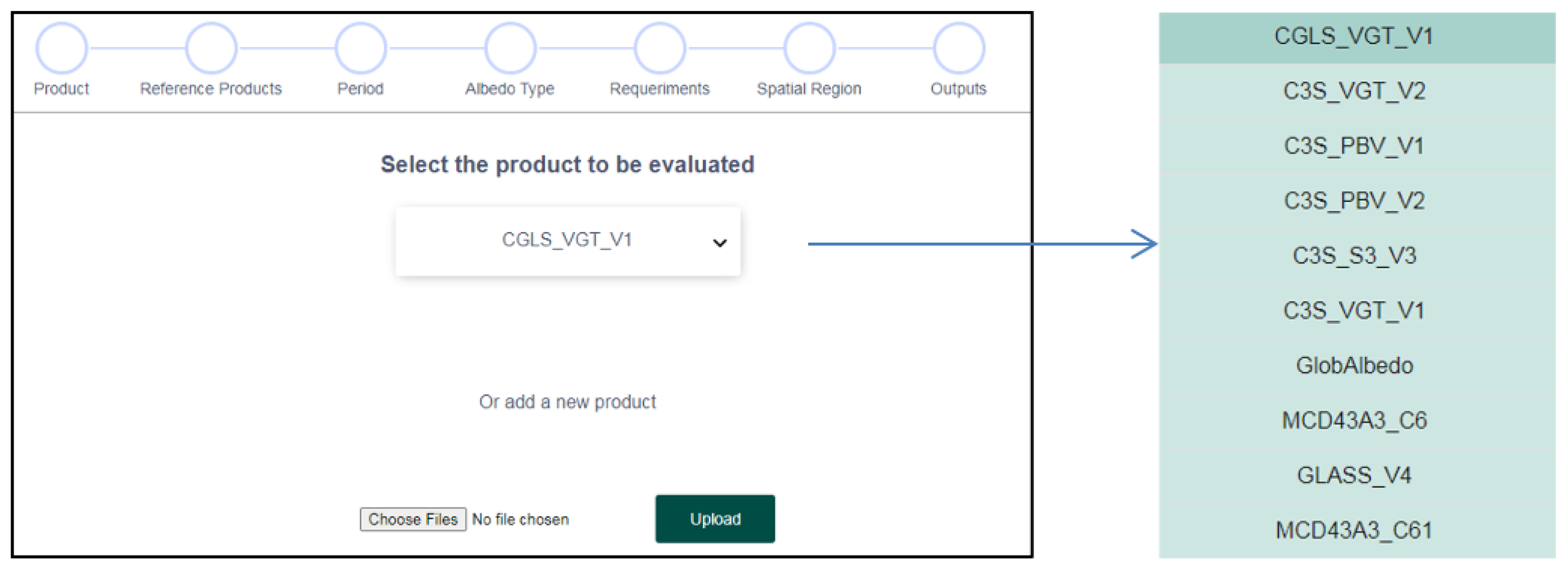
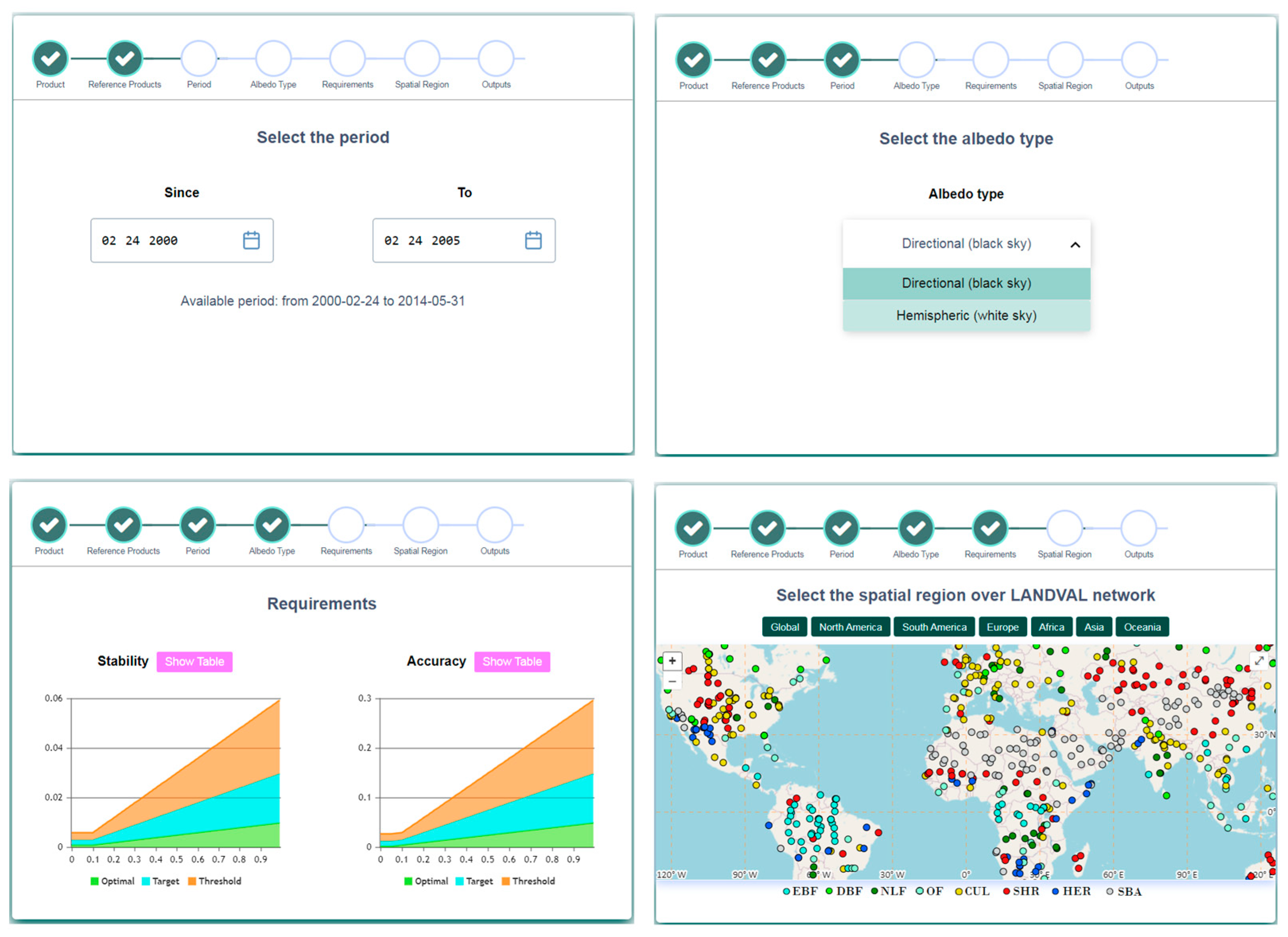
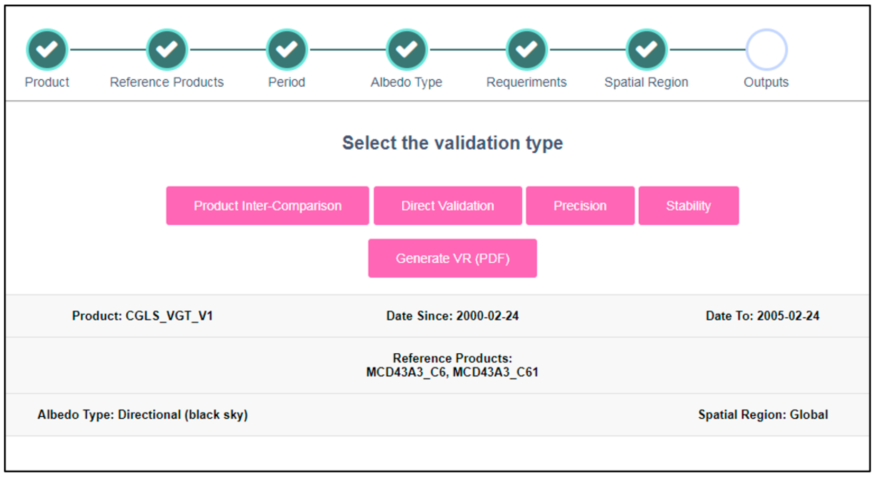
Appendix B. Using the SALVAL Tool
- (1)
- Sign up to start using the SALVAL Tool.

- (2)
- Specify the product being validated and the reference products. Select from the existing database of products or import new products.

- (3)
- Define the input product: time period, albedo type, requirements, and spatial coverage.

- (4)
- Visualize the validation results for different criteria, or generate a standardized validation report in PDF.

- (5)
- Enjoy the interactive validation process (see below Direct Validation type results).
References
- Dickinson, R.E. Land processes in climate models. Remote Sens. Environ. 1995, 51, 27–38. [Google Scholar] [CrossRef]
- Liang, S. A direct algorithm for estimating land surface broadband albedos from MODIS imagery. IEEE Trans. Geosci. Remote Sens. 2003, 41, 136–145. [Google Scholar] [CrossRef]
- WMO; United Nations Educational, Scientific and Cultural Organization; Intergovernmental Oceanographic Commission; United Nations Environment Programme; International Science Council. The 2022 GCOS Implementation Plan (GCOS-244). Available online: https://gcos.wmo.int/en/publications/gcos-implementation-plan2022 (accessed on 10 November 2022).
- Zhou, Y.; Wang, D.; Liang, S.; Yu, Y.; He, T. Assessment of the Suomi NPP VIIRS Land Surface Albedo Data Using Station Measurements and High-Resolution Albedo Maps. Remote Sens. 2016, 8, 137. [Google Scholar] [CrossRef]
- Wang, D.; Liang, S.; Zhou, Y.; He, T.; Yu, Y. A New Method for Retrieving Daily Land Surface Albedo from VIIRS Data. IEEE Trans. Geosci. Remote Sens. 2017, 55, 1765–1775. [Google Scholar] [CrossRef]
- Wang, D.; Liang, S.; He, T.; Yu, Y. Direct estimation of land surface albedo from VIIRS data: Algorithm improvement and preliminary validation. J. Geophys. Res. Atmos. 2013, 118, 12577–12586. [Google Scholar] [CrossRef]
- Balsamo, G.; Agusti-Panareda, A.; Albergel, C.; Arduini, G.; Beljaars, A.; Bidlot, J.; Bousserez, N.; Boussetta, S.; Brown, A.; Buizza, R.; et al. Satellite and In Situ Observations for Advancing Global Earth Surface Modelling: A Review. Remote Sens. 2018, 10, 2038. [Google Scholar] [CrossRef]
- Bayat, B.; Camacho, F.; Nickeson, J.; Cosh, M.; Bolten, J.; Vereecken, H.; Montzka, C. Toward operational validation systems for global satellite-based terrestrial essential climate variables. Int. J. Appl. Earth Obs. Geoinf. 2021, 95, 102240. [Google Scholar] [CrossRef]
- Leroy, M.; Deuzé, J.L.; Bréon, F.M.; Hautecoeur, O.; Herman, M.; Buriez, J.C.; Tanré, D.; Bouffiès, S.; Chazette, P.; Roujean, J.L. Retrieval of atmospheric properties and surface bidirectional reflectances over land from POLDER/ADEOS. J. Geophys. Res. Atmos. 1997, 102, 17023–17037. [Google Scholar] [CrossRef]
- Schaaf, C.B.; Gao, F.; Strahler, A.H.; Lucht, W.; Li, X.; Tsang, T.; Strugnell, N.C.; Zhang, X.; Jin, Y.; Muller, J.P.; et al. First operational BRDF, albedo nadir reflectance products from MODIS. Remote Sens. Environ. 2002, 83, 135–148. [Google Scholar] [CrossRef]
- Strahler, A.H.; Muller, J.-P.; MODIS Science Team Members. MODIS BRDF/Albedo Product: Algorithm Theoretical Basis Document Version 5.0. Available online: https://modis.gsfc.nasa.gov/data/atbd/atbd_mod09.pdf (accessed on 15 February 2023).
- Geiger, B.; Carrer, D.; Franchistéguy, L.; Roujean, J.L.; Meurey, C. Land surface albedo derived on a daily basis from meteosat second generation observations. IEEE Trans. Geosci. Remote Sens. 2008, 46, 3841–3856. [Google Scholar] [CrossRef]
- Carrer, D.; Roujean, J.L.; Meurey, C. Comparing operational MSG/SEVIRI Land Surface albedo products from Land SAF with ground measurements and MODIS. IEEE Trans. Geosci. Remote Sens. 2010, 48, 1714–1728. [Google Scholar] [CrossRef]
- Carrer, D.; Pinault, F.; Lellouch, G.; Trigo, I.F.; Benhadj, I.; Camacho, F.; Ceamanos, X.; Moparthy, S.; Munoz-Sabater, J.; Schüller, L.; et al. Surface Albedo Retrieval from 40-Years of Earth Observations through the EUMETSAT/LSA SAF and EU/C3S Programmes: The Versatile Algorithm of PYALUS. Remote Sens. 2021, 13, 372. [Google Scholar] [CrossRef]
- Lellouch, G.; Carrer, D.; Vincent, C.; Pardé, M.; Frietas, S.C.; Trigo, I.F. Evaluation of Two Global Land Surface Albedo Datasets Distributed by the Copernicus Climate Change Service and the EUMETSAT LSA-SAF. Remote Sens. 2020, 12, 1888. [Google Scholar] [CrossRef]
- Carrer, D.; Moparthy, S.; Lellouch, G.; Ceamanos, X.; Pinault, F.; Freitas, S.C.; Trigo, I.F. Land surface albedo derived on a ten daily basis from Meteosat Second Generation Observations: The NRT and climate data record collections from the EUMETSAT LSA SAF. Remote Sens. 2018, 10, 1262. [Google Scholar] [CrossRef]
- Trigo, I.F.; Dacamara, C.C.; Viterbo, P.; Roujean, J.-L.; Olesen, F.; Barroso, C.; Camacho-de-Coca, F.; Carrer, D.; Freitas, S.C.; García-Haro, J.; et al. The Satellite Application Facility for Land Surface Analysis. Int. J. Remote Sens. 2011, 32, 2725–2744. [Google Scholar] [CrossRef]
- Land Surface Analysis (LSA-SAF) of EUMETSAT. Available online: https://landsaf.ipma.pt/en/ (accessed on 10 November 2022).
- Copernicus Global Land Service (CGLS) portal. Available online: https://land.copernicus.eu/global/index.html (accessed on 10 November 2022).
- Copernicus Climate Change Service (C3S). Available online: https://climate.copernicus.eu/ (accessed on 10 November 2022).
- Sanchez-Zapero, J.; Camacho, F.; Leon-Tavares, J.; Martinez-Sanchez, E.; Gorrono, J.; Benhadj, I.; Tote, C.; Swinnen, E.; Munoz-Sabater, J. Prototype for Surface Albedo Retrieval Based on Sentinel-3 OLCI and SLSTR Data in the Framework of Copernicus Climate Change. In Proceedings of the 2021 IEEE International Geoscience and Remote Sensing Symposium IGARSS, Brussels, Belgium, 11–16 July 2021; pp. 2377–2380. [Google Scholar]
- Liu, Q.; Wang, L.; Qu, Y.; Liu, N.; Liu, S.; Tang, H.; Liang, S. Preliminary evaluation of the long-term GLASS albedo product. Int. J. Digit. Earth 2013, 6, 69–95. [Google Scholar] [CrossRef]
- Liu, Y.; Wang, Z.; Sun, Q.; Erb, A.M.; Li, Z.; Schaaf, C.B.; Zhang, X.; Román, M.O.; Scott, R.L.; Zhang, Q.; et al. Evaluation of the VIIRS BRDF, Albedo and NBAR products suite and an assessment of continuity with the long term MODIS record. Remote Sens. Environ. 2017, 201, 256–274. [Google Scholar] [CrossRef]
- Sánchez-Zapero, J.; Camacho, F.; Martínez-Sánchez, E.; Lacaze, R.; Carrer, D.; Pinault, F.; Benhadj, I.; Muñoz-Sabater, J. Quality Assessment of PROBA-V Surface Albedo V1 for the Continuity of the Copernicus Climate Change Service. Remote Sens. 2020, 12, 2596. [Google Scholar] [CrossRef]
- Zeng, Y.; Su, Z.; Calvet, J.C.; Manninen, T.; Swinnen, E.; Schulz, J.; Roebeling, R.; Poli, P.; Tan, D.; Riihelä, A.; et al. Analysis of current validation practices in Europe for space-based climate data records of essential climate variables. Int. J. Appl. Earth Obs. Geoinf. 2015, 42, 150–161. [Google Scholar] [CrossRef]
- Nightingale, J.; Mittaz, J.P.D.; Douglas, S.; Dee, D.; Ryder, J.; Taylor, M.; Old, C.; Dieval, C.; Fouron, C.; Duveau, G.; et al. Ten Priority Science Gaps in Assessing Climate Data Record Quality. Remote Sens. 2019, 11, 986. [Google Scholar] [CrossRef]
- LPV (Land Product Validation). Subgroup CEOS Validation Hierarchy 2019. Available online: https://lpvs.gsfc.nasa.gov/ (accessed on 2 March 2022).
- Justice, C.; Belward, A.; Morisette, J.; Lewis, P.; Privette, J.; Baret, F. Developments in the’validation’of satellite sensor products for the study of the land surface. Int. J. Remote Sens. 2000, 21, 3383–3390. [Google Scholar] [CrossRef]
- Wang, Z.; Schaaf, C.; Lattanzio, A.; Carrer, D.; Grant, I.; Roman, M.; Camacho, F.; Yang, Y.; Sánchez-Zapero, J. Global Surface Albedo Product Validation Best Practices Protocol. Version 1.0. In Good Practices for Satellite-Derived Land Product Validation (p. 45): Land Product Validation Subgroup (WGCV/CEOS); Wang, Z., Nickeson, J., Román, M., Eds.; Available online: https://lpvs.gsfc.nasa.gov/PDF/CEOS_ALBEDO_Protocol_20190307_v1.pdf (accessed on 1 March 2022).
- Nightingale, J.; Schaepman-Strub, G.; Nickeson, J.; Baret, F.; Herold, M. Assessing Satellite-Derived Land Product Quality for Earth System Science Applications: Overview of the CEOS LPV Sub-Group. In Proceedings of the 34th International Symposium on Remote Sensing of Environment, Sydney, NSW, Australia, 10–15 April 2011. [Google Scholar]
- Mayr, S.; Kuenzer, C.; Gessner, U.; Klein, I.; Rutzinger, M. Validation of Earth Observation Time-Series: A Review for Large-Area and Temporally Dense Land Surface Products. Remote Sens. 2019, 11, 2616. [Google Scholar] [CrossRef]
- Liang, S.; Fang, H.; Chen, M.; Shuey, C.J.; Walthall, C.; Daughtry, C.; Morisette, J.; Schaaf, C.; Strahler, A. Validating MODIS land surface reflectance and albedo products: Methods and preliminary results. Remote Sens. Environ. 2002, 83, 149–162. [Google Scholar] [CrossRef]
- Cescatti, A.; Marcolla, B.; Santhana Vannan, S.K.; Pan, J.Y.; Román, M.O.; Yang, X.; Ciais, P.; Cook, R.B.; Law, B.E.; Matteucci, G.; et al. Intercomparison of MODIS albedo retrievals and in situ measurements across the global FLUXNET network. Remote Sens. Environ. 2012, 121, 323–334. [Google Scholar] [CrossRef]
- EOLAB. Surface ALbedo VALidation (SALVAL) Tool. Available online: https://salval.eolab.es/ (accessed on 10 November 2022).
- JCGM-GUM Joint Committee for Guides in Metrology (JCGM)—Guides to the Expression of Uncertainty in Measurement (GUM). [ISO/IEC Guide 98—Part 3, 2008]. Available online: https://www.iso.org/sites/JCGM/GUM-introduction.htm (accessed on 10 November 2022).
- GCOS-154 Systematic Observation Requirements for Satellite-Based Data Products for Climate. Supplemental Details to the Satellite-Based Component of the “Implementation Plan for the GCOS in Support of the UNFCCC”. Available online: https://library.wmo.int/doc_num.php?explnum_id=3710 (accessed on 10 April 2022).
- SALVAL Sampling—CalValPortal. Available online: https://calvalportal.ceos.org/sampling (accessed on 19 December 2022).
- Camacho, F.; Cernicharo, J.; Lacaze, R.; Baret, F.; Weiss, M. GEOV1: LAI, FAPAR essential climate variables and FCOVER global time series capitalizing over existing products. Part 2: Validation and intercomparison with reference products. Remote Sens. Environ. 2013, 137, 310–329. [Google Scholar] [CrossRef]
- Sánchez, J.; Camacho, F.; Lacaze, R.; Smets, B. Early validation of PROBA-V GEOV1 LAI, FAPAR and FCOVER products for the continuity of the copernicus global land service. Int. Arch. Photogramm. Remote Sens. Spat. Inf. Sci.—ISPRS Arch. 2015, 40, 93–100. [Google Scholar] [CrossRef]
- Lewis, P.; Barnsley, M. Influence of the sky radiance distribution on various formulations of the earth surface albedo. In Proceedings of the 6th International Symposium on Physical Measurements and Signatures in Remote Sensing, ISPRS, Val d’Isère, France, 17–22 January 1994; pp. 707–715. [Google Scholar]
- Román, M.O.; Schaaf, C.B.; Woodcock, C.E.; Strahler, A.H.; Yang, X.; Braswell, R.H.; Curtis, P.S.; Davis, K.J.; Dragoni, D.; Goulden, M.L.; et al. The MODIS (Collection V005) BRDF/albedo product: Assessment of spatial representativeness over forested landscapes. Remote Sens. Environ. 2009, 113, 2476–2498. [Google Scholar] [CrossRef]
- Román, M.O.; Schaaf, C.B.; Lewis, P.; Gao, F.; Anderson, G.P.; Privette, J.L.; Strahler, A.H.; Woodcock, C.E.; Barnsley, M. Assessing the coupling between surface albedo derived from MODIS and the fraction of diffuse skylight over spatially-characterized landscapes. Remote Sens. Environ. 2010, 114, 738–760. [Google Scholar] [CrossRef]
- MODIS Data Products. Available online: https://modis.gsfc.nasa.gov/data/dataprod/ (accessed on 10 November 2022).
- Global LAnd Surface Satellite (GLASS). Available online: http://www.glass.umd.edu/ (accessed on 1 April 2022).
- Globalbedo Portal. Available online: http://www.globalbedo.org/ (accessed on 10 November 2022).
- Schaepman-Strub, G.; Schaepman, M.E.; Painter, T.H.; Dangel, S.; Martonchik, J.V. Reflectance quantities in optical remote sensing-definitions and case studies. Remote Sens. Environ. 2006, 103, 27–42. [Google Scholar] [CrossRef]
- Lucht, W.; Schaaf, C.B.; Strahler, A.H. An algorithm for the retrieval of albedo from space using semiempirical BRDF models. IEEE Trans. Geosci. Remote Sens. 2000, 38, 977–998. [Google Scholar] [CrossRef]
- Shuai, Y.; Tuerhanjiang, L.; Shao, C.; Gao, F.; Zhou, Y.; Xie, D.; Liu, T.; Liang, J.; Chu, N. Re-understanding of land surface albedo and related terms in satellite-based retrievals. Big Earth Data 2020, 4, 45–67. [Google Scholar] [CrossRef]
- Schaaf, C.; Wang, Z. MODIS/Terra+Aqua BRDF/Albedo Daily L3 Global—500m V061 [Data set]. NASA EOSDIS Land Processes DAAC. Available online: https://lpdaac.usgs.gov/products/mcd43a3v061/ (accessed on 20 December 2022).
- Lucht, W.; Lewis, P. Theoretical noise sensitivity of BRDF and albedo retrieval from the EOS-MODIS and MISR sensors with respect to angular sampling. Int. J. Remote Sens. 2000, 21, 81–98. [Google Scholar] [CrossRef]
- Sun, Q.; Wang, Z.; Li, Z.; Erb, A.; Schaaf, C.B. Evaluation of the global MODIS 30 arc-second spatially and temporally complete snow-free land surface albedo and reflectance anisotropy dataset. Int. J. Appl. Earth Obs. Geoinf. 2017, 58, 36–49. [Google Scholar] [CrossRef]
- Liang, S.A.H.S.C.W. Retrieval of Land Surface Albedo from Satellite Observations: A Simulation Study. J. Appl. Meteorol. 1999, 38, 712–725. [Google Scholar] [CrossRef]
- Wang, Z.; Schaaf, C.B.; Sun, Q.; Shuai, Y.; Román, M.O. Capturing rapid land surface dynamics with Collection V006 MODIS BRDF/NBAR/Albedo (MCD43) products. Remote Sens. Environ. 2018, 207, 50–64. [Google Scholar] [CrossRef]
- Wang, Z.; Schaaf, C.B.; Chopping, M.J.; Strahler, A.H.; Wang, J.; Román, M.O.; Rocha, A.V.; Woodcock, C.E.; Shuai, Y. Evaluation of Moderate-resolution Imaging Spectroradiometer (MODIS) snow albedo product (MCD43A) over tundra. Remote Sens. Environ. 2012, 117, 264–280. [Google Scholar] [CrossRef]
- Wang, Z.; Schaaf, C.B.; Strahler, A.H.; Chopping, M.J.; Román, M.O.; Shuai, Y.; Woodcock, C.E.; Hollinger, D.Y.; Fitzjarrald, D.R. Evaluation of MODIS albedo product (MCD43A) over grassland, agriculture and forest surface types during dormant and snow-covered periods. Remote Sens. Environ. 2014, 140, 60–77. [Google Scholar] [CrossRef]
- Climate Data Store of Copernicus Climate Change Service. Available online: https://cds.climate.copernicus.eu/#!/home (accessed on 10 May 2020).
- Carrer, D.; Pinault, F.; Ramon, D.; Benhadj, I.; Swinnen, E. Algorithm Theoretical Basis Document (ATBD) of CDR SPOT/VGT Surface Albedo v1.0 (Official Reference Number Service Contract: 2018/C3S_312b_Lot5_VITO/SC1). Available online: https://datastore.copernicus-climate.eu/documents/satellite-albedo/D1.3.3-v1.0_ATBD_CDR-ICDR_SA_PROBAV_v1.0_PRODUCTS_v1.0.2.pdf (accessed on 1 November 2022).
- Carrer, D.; Pinault, F.; Bigeard, G.; Ramon, D.; Jolivet, D.; Kirches, G.; Brockmann, C.; Boettcher, M.; Benhadj, I. Algorithm Theoretical Basis Document Multi sensor CDR Surface Albedo v2.0 (Official Reference Number Service Contract: 2018/C3S_312b_Lot5_VITO/SC1). Available online: https://datastore.copernicus-climate.eu/documents/satellite-albedo/D1.3.4-v2.0_ATBD_CDR_SA_MULTI_SENSOR_v2.0_PRODUCTS_v1.1.pdf (accessed on 10 November 2022).
- Rahman, H.; Dedieu, G. SMAC: A simplified method for the atmospheric correction of satellite measurements in the solar spectrum. Int. J. Remote Sens. 1994, 15, 123–143. [Google Scholar] [CrossRef]
- Sánchez-Zapero, J.; Martínez-Sánchez, E.; Camacho, F.; León-Tavares, J. Product Quality Assessment Report Multi-sensor Surface Albedo v2.0 (Official Reference Number Service Contract: 2018/C3S_312b_Lot5_VITO/SC1). Available online: https://datastore.copernicus-climate.eu/documents/satellite-albedo/D2.3.4-v2.0_PQAR_CDR_SA_MULTI_SENSOR_v2.0_PRODUCTS_v1.1.pdf (accessed on 10 November 2022).
- Liang, S.; Cheng, J.; Jia, K.; Jiang, B.; Liu, Q.; Xiao, Z.; Yao, Y.; Yuan, W.; Zhang, X.; Zhao, X.; et al. The Global LAnd Surface Satellite (GLASS) product suite. Bull. Am. Meteorol. Soc. 2020, 102, E323–E337. [Google Scholar] [CrossRef]
- Qu, Y.; Liu, Q.; Liang, S.; Wang, L.; Liu, N.; Liu, S. Direct-estimation algorithm for mapping daily land-surface broadband albedo from modis data. IEEE Trans. Geosci. Remote Sens. 2014, 52, 907–919. [Google Scholar] [CrossRef]
- Liu, N.F.; Liu, Q.; Wang, L.Z.; Liang, S.L.; Wen, J.G.; Qu, Y.; Liu, S.H. A statistics-based temporal filter algorithm to map spatiotemporally continuous shortwave albedo from MODIS data. Hydrol. Earth Syst. Sci. 2013, 17, 2121–2129. [Google Scholar] [CrossRef]
- Qu, Y.; Liang, S.; Liu, Q.; Li, X.; Feng, Y.; Liu, S. Estimating Arctic sea-ice shortwave albedo from MODIS data. Remote Sens. Environ. 2016, 186, 32–46. [Google Scholar] [CrossRef]
- Feng, Y.; Liu, Q.; Qu, Y.; Liang, S. Estimation of the Ocean Water Albedo From Remote Sensing and Meteorological Reanalysis Data. IEEE Trans. Geosci. Remote Sens. 2016, 54, 850–868. [Google Scholar] [CrossRef]
- Ground-Based Observations for Validation (GBOV) of Copernicus Global Land Products Site. Available online: https://land.copernicus.eu/global/gbov (accessed on 3 November 2022).
- FLUXNET. The Data Portal serving the FLUXNET Community. Available online: https://fluxnet.org/ (accessed on 10 November 2022).
- NSF NEON. Open Data to Understand our Ecosystems. Available online: https://www.neonscience.org/ (accessed on 10 November 2022).
- European Fluxes Database Cluster. Available online: http://www.europe-fluxdata.eu/ (accessed on 10 November 2022).
- ICOS—Integrated Carbon Observation System. Available online: https://www.icos-cp.eu/ (accessed on 10 November 2022).
- TERN—Australia’s Terrestrial Ecosystem Research Network. Available online: https://www.tern.org.au/ (accessed on 10 November 2022).
- Ohmura, A.; Dutton, E.G.; Forgan, B.; Fröhlich, C.; Gilgen, H.; Hegner, H.; Heimo, A.; König-Langlo, G.; McArthur, B.; Müller, G.; et al. Baseline Surface Radiation Network (BSRN/WCRP): New Precision Radiometry for Climate Research. Bull. Am. Meteorol. Soc. 1998, 79, 2115–2136. [Google Scholar] [CrossRef]
- ESRL Global Monitoring Laboratory—Global Radiation and Aerosols. SURFRAD. Available online: https://gml.noaa.gov/grad/surfrad/ (accessed on 20 December 2022).
- Matheron, G. Principles of geostatistics. Econ. Geol. 1963, 58, 1246–1266. [Google Scholar] [CrossRef]
- Hohn, M.E. An Introduction to Applied Geostatistics: By Edward H. Isaaks and R. Mohan Srivastava, 1989, Oxford University Press, New York, 561 p., ISBN 0-19-505012-6, ISBN 0-19-505013-4. Comput. Geosci. 1991, 17, 471–473. [Google Scholar] [CrossRef]
- Copernicus Sentinel-2 Mission. Available online: https://sentinel.esa.int/web/sentinel/missions/sentinel-2 (accessed on 20 December 2022).
- Bonafoni, S.; Sekertekin, A. Albedo Retrieval from Sentinel-2 by New Narrow-to-Broadband Conversion Coefficients. IEEE Geosci. Remote Sens. Lett. 2020, 17, 1618–1622. [Google Scholar] [CrossRef]
- Ohring, G.; Wielicki, B.; Spencer, R.; Emery, B.; Datla, R. Satellite Instrument Calibration for Measuring Global Climate Change: Report of a Workshop. Bull. Am. Meteorol. Soc. 2005, 86, 1303–1314. [Google Scholar] [CrossRef]
- World Meteorological Organization (WMO) Requirements for Earth Surface Albedo. Available online: https://www.wmo-sat.info/oscar/variables/view/54 (accessed on 10 April 2020).
- The 2022 GCOS ECVs Requirements (GCOS 245). Available online: https://library.wmo.int/index.php?lvl=notice_display&id=22135#.Y5eLMofMI2whttps://library.wmo.int/doc_num.php?explnum_id=11318 (accessed on 20 December 2022).
- Sánchez-Zapero, J.; Camacho, F. Product Quality Assessment Report (PQAR) of CDR and ICDR Surface Albedo v1.0 based on PROBA-V (Official Reference Number Service Contract: 2018/C3S_312b_Lot5_VITO/SC1). Available online: https://cds.climate.copernicus.eu/cdsapp#!/dataset/satellite-albedo?tab=doc (accessed on 9 April 2022).
- Iannone, R.Q.; Niro, F.; Goryl, P.; Dransfeld, S.; Hoersch, B.; Stelzer, K.; Kirches, G.; Paperin, M.; Brockmann, C.; Gomez-Chova, L.; et al. Proba-V cloud detection Round Robin: Validation results and recommendations. In Proceedings of the 2017 9th International Workshop on the Analysis of Multitemporal Remote Sensing Images, MultiTemp, Bruges, Belgium, 27–29 June 2017; pp. 1–8. [Google Scholar] [CrossRef]
- Weiss, M.; Baret, F.; Block, T.; Koetz, B.; Burini, A.; Scholze, B.; Lecharpentier, P.; Brockmann, C.; Fernandes, R.; Plummer, S.; et al. On line validation exercise (OLIVE): A web based service for the validation of medium resolution land products. application to FAPAR products. Remote Sens. 2014, 6, 4190–4216. [Google Scholar] [CrossRef]
- Lacherade, S.; Fougnie, B.; Henry, P.; Gamet, P. Cross calibration over desert sites: Description, methodology, and operational implementation. IEEE Trans. Geosci. Remote Sens. 2013, 51, 1098–1113. [Google Scholar] [CrossRef]
- Merchant, C.J. Thermal remote sensing of sea surface temperature. Therm. Infrared Remote Sens. Sens. Methods Appl. 2013, 17, 287–313. [Google Scholar]
- Fell, F.; Bennartz, R.; Loew, A. Validation of the EUMETSAT Geostationary Surface Albedo Climate Data Record -2- (ALBEDOVAL-2). Available online: https://www.eumetsat.int/website/home/Data/TechnicalDocuments/index.html (accessed on 12 April 2020).
- Gu, L.; Shuai, Y.; Shao, C.; Xie, D.; Zhang, Q.; Li, Y.; Yang, J.; Gu, L.; Shuai, Y.; Shao, C.; et al. Angle Effect on Typical Optical Remote Sensing Indices in Vegetation Monitoring. Remote Sens. 2021, 13, 1699. [Google Scholar] [CrossRef]
- Kokhanovsky, A.A.; Breon, F.M. Validation of an analytical snow BRDF model using PARASOL multi-angular and multispectral observations. IEEE Geosci. Remote Sens. Lett. 2012, 9, 928–932. [Google Scholar] [CrossRef]
- Liang, S. Narrowband to broadband conversions of land surface albedo I Algorithms. Remote Sens. Environ. 2001, 76, 213–238. [Google Scholar] [CrossRef]
- CalVal Portal: SALVAL Tool. Available online: https://calvalportal.ceos.org/salval (accessed on 14 November 2022).


| Stage | Description |
|---|---|
| 0 | No validation. Product accuracy has not been assessed. Product considered beta. |
| 1 | Product accuracy is assessed from a small (typically < 30) set of locations and time periods by comparison with in situ or other suitable reference data. |
| 2 | Product accuracy is estimated over a significant (typically > 30) set of locations and time periods by comparison with reference in situ or other suitable reference data. Spatial and temporal consistency of the product, and its consistency with similar products, has been evaluated over globally representative locations and time periods. Results are published in the peer-reviewed literature. |
| 3 | Uncertainties in the product and its associated structure are well quantified over a significant (typically > 30) set of locations and time periods representing global conditions by comparison with reference in situ or other suitable reference data. Validation procedures follow community-agreed-upon good practices. Spatial and temporal consistency of the product, and its consistency with similar products, has been evaluated over globally representative locations and time periods. Results are published in the peer-reviewed literature. |
| 4 | Validation results for stage 3 are systematically updated when new product versions are released or as the inter-annual time series expands. When appropriate for the product, uncertainties in the product are quantified using fiducial reference measurements over a global network of sites and time periods (if available). |
| Category | Criteria | Methods |
|---|---|---|
| Product inter- comparison | Completeness | Gap size distribution (spatial and temporal) and gap length. |
| Spatial consistency | Mean residual and mean difference maps, percentage of cases within requirements | |
| Temporal consistency | Temporal profiles and histograms of cross-correlation | |
| Overall analysis | Product histograms, difference histograms, scatterplots (APU validation metrics) and box plots of bias and Root Mean Square Deviation (RMSD) per bin | |
| Direct validation | Temporal realism | Temporal evolution of the satellite-derived products vs ground data |
| Overall analysis | Scatterplots (APU validation metrics) | |
| Precision | Intra-annual precision | Median 3-point difference (smoothness) |
| Inter-annual precision | Median absolute deviation over desert calibration sites | |
| Stability | Stability | Slope of the 10-year linear regression over desert calibration sites |
| Statistics | Comment |
|---|---|
| N | Number of samples. Indicative of the strength of the validation. |
| B | Mean Bias. Difference between average values of x and y. Indicative of accuracy and offset. Bias (%) is the relative mean bias between the average of x and y. |
| MD | Median (i.e., 50th percentile) deviation between x and y. MD is the CEOS LPV good practice reporting of the accuracy. MD (%) is the relative MD between the average of x and y. |
| STD | Standard deviation of the pair differences. Indicates precision. STD (%) is the relative STD between the average of x and y. |
| MAD | Median (i.e., 50th percentile) absolute deviation between x and y. MAD is the CEOS LPV good practice indicator of precision. MAD (%) is the relative MAD between the average of x and y. |
| RMSD | Root Mean Square Deviation. RMSD is the square root of the average of squared errors between x and y. The RMSD is the CEOS LPV good practice reporting of uncertainty. RMSD (%) is the relative RMSD between the average of x and y. |
| R | Correlation coefficient. Indicates descriptive power of the linear accuracy test. Pearson coefficient is used. |
| MAR | Slope and offset of the Major Axis Regression (MAR) linear fit. Indicates possible bias. |
| Product | Satellite /Sensor | Methodology | Broadband Definition | Frequency /Period | GSD /Projection | Reference |
| NASA MCD43A3 C6.1 | TERRA + AQUA /MODIS | BRDF model inversion and angular/spectral integration | visible [0.3–0.7 μm] NIR [0.7–5.0 μm] total SW [0.3–5.0 μm] | Daily (*) /16 days | 500 m /Sinusoidal | [10] |
| C3S V2 | SPOT /VGT PROBA /VGT | BRDF model inversion and angular/spectral integration | visible [0.4–0.7 µm] NIR [0.7–4 µm] total SW [0.3–4.0 µm] | 10 days /20 days using prior climatology BRDF | 1 km /Plate Carrée | [14,58] |
| GLASS V4 | TERRA + AQUA /MODIS | RTM + gap-filling | visible [0.3–0.7 μm] NIR [0.7–5.0 μm] total SW [0.3–5.0 μm] | 8 days /16 days | 1 km /Sinusoidal | [61] |
| Product | Quality Control Used as “Best Quality” | Quality Control Used to Discard Pixels |
|---|---|---|
| MCD43A2 C6.1 | Full BRDF inversion | Magnitude inversion |
| C3S V2 | Land (bits 0–1 QFLAG) Normally processed (bit 7 QFLAG) ERR 0.2 AGE 20 | Sea and continental water (bits 0–1 QFLAG) Algorithm Failed (bit 7 QFLAG) ERR > 0.2 AGE > 20 |
| GLASS V4 | Overall uncertainty ‘best quality’ | Overall uncertainty ‘acceptable’, ‘with uncertainty’ or ‘fill value’ |
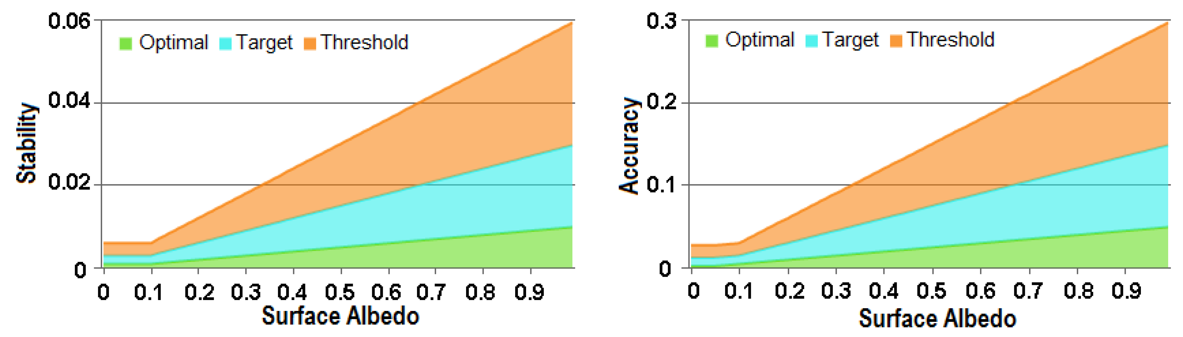
| Optimal | Target | Threshold | |
|---|---|---|---|
| Accuracy requirement | Max [5%, 0.0025] | Max [10%, 0.01] | Max [15%, 0.015] |
| Stability requirement | Max [1%, 0.001] | Max [2%, 0.002] | Max [3%, 0.003] |
| Residual | Optimal | Target | Threshold | Non-Compliance |
|---|---|---|---|---|
| C3S V2 vs. GLASS V4 | 83.5% | 98.1% | 99.7% | 0.3% |
| C3S V2 vs. MCD43A3 C61 | 72.8% | 91.8% | 95.4% | 4.6% |
| GLASS V4 vs. MCD43A3 C61 | 89.6% | 94.5% | 94.9% | 5.1% |
| Satellite Product | Median δ |
|---|---|
| C3S V2 | 0.0022 |
| GLASS V4 | 0.0014 |
| MCD43A3 C6.1 | 0.0008 |
| C3S V2 | GLASS V4 | MCD43A3 C6.1 | |
|---|---|---|---|
| Inter-annual precision: median absolute deviation | 0.007 (1.64%) | 0.002 (0.55%) | 0.004 (0.84%) |
| C3S V2 vs. GLASS V4 | C3S V2 vs. MCD43A3 C6.1 | GLASS V4 vs. MCD43A3 C6.1 | |
|---|---|---|---|
| N | 122086 | 115912 | 145694 |
| R | 0.91 | 0.89 | 0.94 |
| MAR | y = 0.87x + 0.04 | y = 0.83x + 0.05 | y = 0.96x + 0.01 |
| B | 0.017 (8.1%) | 0.015 (7.1%) | −0.001 (−0.3%) |
| MD | 0.024 (11.4%) | 0.024 (11.2%) | <0.001 (0.2%) |
| STD | 0.052 (24.8%) | 0.062 (28.7%) | 0.043 (21.0%) |
| MAD | 0.027 (12.7%) | 0.027 (12.8%) | 0.006 (3.0%) |
| RMSD | 0.055 (26.1%) | 0.064 (29.6%) | 0.043 (21.0%) |
| %Optimal | 10.2 | 9.6 | 61.8 |
| %Target | 28.4 | 29.4 | 83.7 |
| %Threshold | 49.4 | 49.7 | 90.9 |
| C3S V2 vs. GLASS V4 | C3S V2 vs. MCD43A3 C6.1 | GLASS V4 vs. MCD43A3 C6.1 | |
|---|---|---|---|
| N | 102857 | 52954 | 69280 |
| R | 0.90 | 0.99 | 0.97 |
| MAR | y = 0.94x + 0.03 | y = 1.03x + 0.02 | y = 1.01x + 0.00 |
| B | 0.021 (11.0%) | 0.022 (10.6%) | >−0.001 (−0.0%) |
| MD | 0.025 (13.0%) | 0.022 (10.3%) | −0.001 (−0.5%) |
| STD | 0.037 (19.5%) | 0.013 (6.2%) | 0.026 (12.4%) |
| MAD | 0.026 (13.5%) | 0.022 (10.3%) | 0.005 (2.3%) |
| RMSD | 0.042 (22.4%) | 0.026 (12.3%) | 0.026 (12.4%) |
| %Optimal | 9.8 | 12.4 | 77.5 |
| %Target | 28.7 | 43.1 | 95.8 |
| %Threshold | 50.6 | 70.4 | 98.7 |
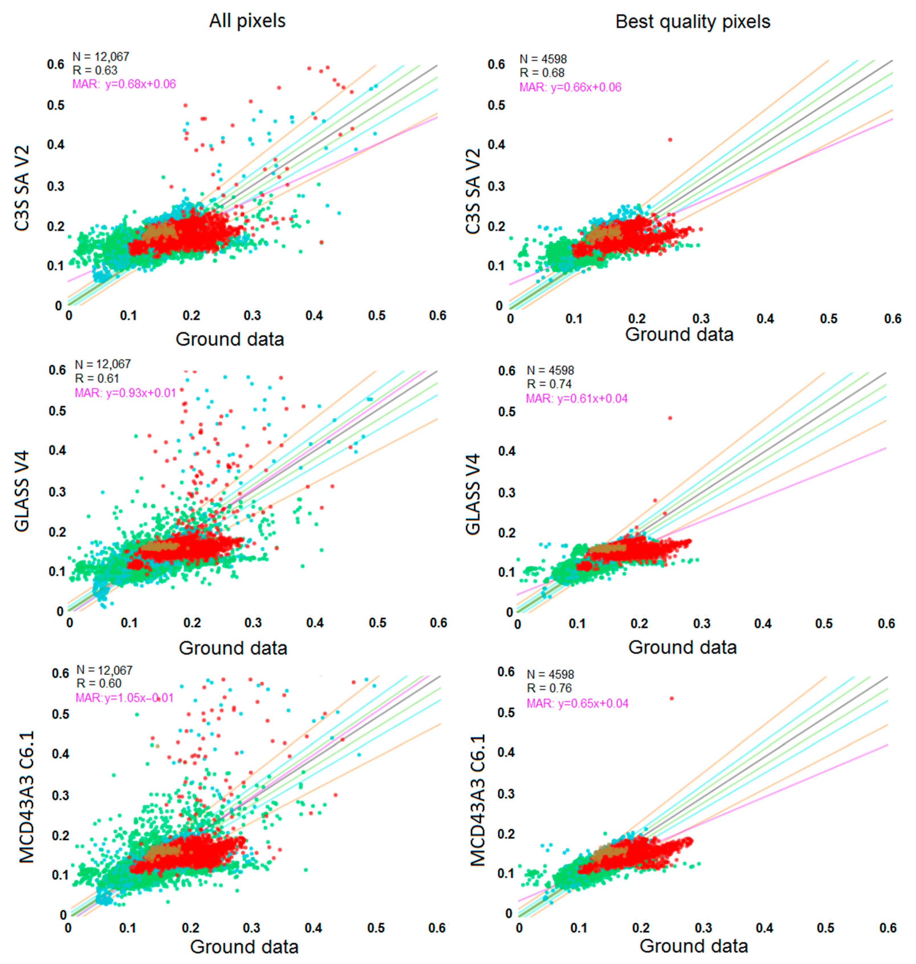
| C3S V2 | GLASS V4 | MCD43A3 C6.1 | |
|---|---|---|---|
| N | 12067 | 12067 | 12067 |
| R | 0.63 | 0.61 | 0.60 |
| MAR | y = 0.68x + 0.06 | y = 0.93x + 0.01 | y = 1.05x−0.01 |
| B | 0.017 (12.2%) | −0.003 (−2.5%) | −0.003 (−2.5%) |
| MD | 0.021 (14.9%) | <0.001 (−0.1%) | −0.002 (−1.2%) |
| STD | 0.040 (27.8%) | 0.043 (32.7%) | 0.047 (35.2%) |
| MAD | 0.029 (20.4%) | 0.017 (13.2%) | 0.017 (13.2%) |
| RMSD | 0.043 (30.4%) | 0.043 (32.8%) | 0.047 (35.3%) |
| %Optimal | 12.6 | 20.6 | 18.1 |
| %Target | 24.5 | 38.3 | 37.0 |
| %Threshold | 46.8 | 63.1 | 64.7 |
| C3S V2 | GLASS V4 | MCD43A3 C6.1 | |
|---|---|---|---|
| N | 4598 | 4598 | 4598 |
| R | 0.68 | 0.74 | 0.76 |
| MAR | y =0.66x + 0.06 | y = 0.61x + 0.04 | y = 0.65x + 0.04 |
| B | 0.014 (9.7%) | −0.008 (−6.2%) | −0.008 (−5.7%) |
| MD | 0.017 (11.7%) | −0.004 (−2.9%) | −0.005 (−3.8%) |
| STD | 0.032 (22.2%) | 0.030 (22.3%) | 0.029 (21.6%) |
| MAD | 0.024 (16.7%) | 0.013 (10.1%) | 0.015 (11.3%) |
| RMSD | 0.035 (24.2%) | 0.031 (23.2%) | 0.030 (22.4%) |
| %Optimal | 16.8 | 27.5 | 20.9 |
| %Target | 32.2 | 48.1 | 43.3 |
| %Threshold | 56.8 | 72.0 | 73.4 |
Disclaimer/Publisher’s Note: The statements, opinions and data contained in all publications are solely those of the individual author(s) and contributor(s) and not of MDPI and/or the editor(s). MDPI and/or the editor(s) disclaim responsibility for any injury to people or property resulting from any ideas, methods, instructions or products referred to in the content. |
© 2023 by the authors. Licensee MDPI, Basel, Switzerland. This article is an open access article distributed under the terms and conditions of the Creative Commons Attribution (CC BY) license (https://creativecommons.org/licenses/by/4.0/).
Share and Cite
Sánchez-Zapero, J.; Martínez-Sánchez, E.; Camacho, F.; Wang, Z.; Carrer, D.; Schaaf, C.; García-Haro, F.J.; Nickeson, J.; Cosh, M. Surface ALbedo VALidation (SALVAL) Platform: Towards CEOS LPV Validation Stage 4—Application to Three Global Albedo Climate Data Records. Remote Sens. 2023, 15, 1081. https://doi.org/10.3390/rs15041081
Sánchez-Zapero J, Martínez-Sánchez E, Camacho F, Wang Z, Carrer D, Schaaf C, García-Haro FJ, Nickeson J, Cosh M. Surface ALbedo VALidation (SALVAL) Platform: Towards CEOS LPV Validation Stage 4—Application to Three Global Albedo Climate Data Records. Remote Sensing. 2023; 15(4):1081. https://doi.org/10.3390/rs15041081
Chicago/Turabian StyleSánchez-Zapero, Jorge, Enrique Martínez-Sánchez, Fernando Camacho, Zhuosen Wang, Dominique Carrer, Crystal Schaaf, Francisco Javier García-Haro, Jaime Nickeson, and Michael Cosh. 2023. "Surface ALbedo VALidation (SALVAL) Platform: Towards CEOS LPV Validation Stage 4—Application to Three Global Albedo Climate Data Records" Remote Sensing 15, no. 4: 1081. https://doi.org/10.3390/rs15041081
APA StyleSánchez-Zapero, J., Martínez-Sánchez, E., Camacho, F., Wang, Z., Carrer, D., Schaaf, C., García-Haro, F. J., Nickeson, J., & Cosh, M. (2023). Surface ALbedo VALidation (SALVAL) Platform: Towards CEOS LPV Validation Stage 4—Application to Three Global Albedo Climate Data Records. Remote Sensing, 15(4), 1081. https://doi.org/10.3390/rs15041081