Article

Assessing the Use of Sentinel-2 Data for Spatio-Temporal Upscaling of Flux Tower Gross Primary Productivity Measurements

by
Anna Spinosa
1,2,*,
Mario Alberto Fuentes-Monjaraz
1 and
Ghada El Serafy
1,2
1
Stitching Deltares, Boussinesqweg 1, 2629 HV Delft, The Netherlands
2
Delft Institute of Applied Mathematics, Electrical Engineering, Mathematics and Computer Science (EEMCS), Technical University of Delft, Mekelweg 4, 2628 CD Delft, The Netherlands
*
Author to whom correspondence should be addressed.
Remote Sens. 2023, 15(3), 562; https://doi.org/10.3390/rs15030562
Submission received: 14 December 2022 / Revised: 12 January 2023 / Accepted: 14 January 2023 / Published: 17 January 2023
(This article belongs to the Special Issue Earth Observations for Sustainable Development Goals)

Abstract

:
The conservation, restoration and sustainable use of wetlands is the target of several international agreements, among which are the Sustainable Development Goals (SDGs). Earth Observation (EO) technologies can assist national authorities in monitoring activities and the environmental status of wetlands to achieve these targets. In this study, we assess the capabilities of the Sentinel-2 instrument to model Gross Primary Productivity (GPP) as a proxy for the monitoring of ecosystem health. To estimate the spatial and temporal variation of GPP, we develop an empirical model correlating in situ measurements of GPP, eight Sentinel-2 derived vegetation indexes (VIs), and different environmental drivers of GPP. The model automatically performs an interdependency analysis and selects the model with the highest accuracy and statistical significance. Additionally, the model is upscaled across larger areas and monthly maps of GPP are produced. The study methodology is applied in a marsh ecosystem located in Doñana National Park, Spain. In this application, a combination of the red-edge chlorophyll index (CLr) and rainfall data results in the highest correlation with in situ measurements of GPP and is used for the model formulation. This yields a coefficient of determination (R2) of 0.93, Mean Absolute Error (MAE) equal to 0.52 gC m−2 day−1, Root Mean Squared Error (RMSE) equal to 0.63 gC m−2 day−1, and significance level p < 0.05. The model outputs are compared with the MODIS GPP global product (MOD17) for reference; an enhancement of the estimation of GPP is found in the applied methodology.

Graphical Abstract

1. Introduction

Healthy ecosystems are a primary source of vital resources for human welfare and survival while regulating the impacts of natural hazards and protecting human settlements against floods, landslides, and drought events, thus playing a key role in mitigating climate change effects [1]. Conserving biodiversity and preventing biodiversity shifts is, therefore, of significant importance and a main target of multiple international conventions. The Sustainable Development Goals (SDGs) [2] and the Paris Agreement by the United Nations Framework Convention on Climate Change (UNFCCC) [3] promote the conservation of ecosystems and their associated biodiversity. The conservation, restoration and sustainable use of ecosystems are specifically mentioned in SDG 6.6 and SDG 15.1. The first, SDG 6.6, aims to “protect and restore water-related ecosystems, including mountains, forests, wetlands, rivers, aquifers and lakes”, while SDG 15.1 aims at ensuring “the conservation, restoration and sustainable use of terrestrial and inland freshwater ecosystems and their services, in particular forests, wetlands, mountains and drylands, in line with obligations under international agreements”. Other agreements and commitments include the Aichi Biodiversity Targets by Parties of the United Nations (UN) and the Convention on Biological Diversity (CBD) [4,5].
Providing information on the health of ecosystems status through monitoring activities is essential for applying suitable conservation and restoration practices. In recent years, Earth Observation (EO) technologies, particularly Satellite Remote Sensing (SRS), have been used to assist national authorities in monitoring programs for the achievement of the SDGs [6]. The main advantages of SRS include the provision of data in a systematic and timely way, the cost-effectiveness of monitoring activities and accessibility to remote areas [7,8,9]. SRS can capture biodiversity changes both at global and regional scales [10,11], thus the joint use of SRS data with in situ data and images obtained from other technologies (Light Detection and Ranging (LiDAR), Unmanned Aerial Vehicle (UAV), etc.) is a key factor to generate actionable knowledge in real-time for improved decision-making [10].
To generate actionable knowledge, SRS data need to be translated into information and specifics metrics, maps, or consumable information products that can then be used to inform decision-makers. Structural and functional indicators are both required to evaluate the ecosystem’s health. Structural indicators reflect on the extension and composition of the ecosystems; functional indicators are useful to understand whether the areas are fulfilling their ecosystem role [12]. Structural indicators are often used in monitoring programs whereas ecosystem functions are rarely measured [13,14,15,16], although they are sensitive indicators of ecosystem health [17] and losses of biodiversity [18]. Ecosystem functions are the aggregation of multiple processes that overall define the ecosystem’s capacity to bring benefits to a range of species [9,19]. Among these components, is Primary Productivity (PP). PP can be categorized into Gross Primary Production (GPP), the total amount of carbon or energy captured by plants and Net Primary Production (NPP), the carbon allocated to plant tissue after accounting for the costs of autotrophic respiration. PP is a process that underpins most of the ecosystem functions essential for the understanding of the global carbon cycle [20]. Due to its relevance in the characterization of biodiversity change, PP is considered an Essential Biodiversity Variable (EBV). EBVs are defined as the derived measurements to study and manage biodiversity change, and their estimation is a step forward for integral monitoring programs and holistic health assessments in ecosystems [4,21].
PP has been widely related to the Vegetation Indexes (VIs), used as a proxy for vegetation productivity and to create long-term and consistent data series. Since their first use in the early 1970s, VIs have evolved rapidly together with the increased number of spectral bands of the sensors and the new demand for measuring specific ecological indicators [7]. Particularly, the Normalized Difference Vegetation Index (NDVI) and the Enhanced Vegetation Index (EVI) have been widely used for the monitoring of primary productivity. Empirical models linking the NDVI and EVI with GPP or NPP in situ observations have shown accurate NDVI-GPP correlation in low biomass vegetation areas [9,22] and good performance of the EVI in high biomass vegetated areas such as dense grass or forest ecosystems [23,24]. Additional VIs have also been investigated, such as the two-band Enhanced Vegetation Index (EVI2) used by Cai et al. to assess the relationship between the EVI2, meteorological variables and GPP within the Nordic region [25]. A recently suggested vegetation index, the Near-Infrared Reflectance of terrestrial vegetation (NIRv) [26] has also shown a high correlation with GPP across different ecosystems [27,28] and temporal scales [29,30]. Recent outcomes in research suggest that given that GPP is not only connected to the greenest of vegetation, but also to other processes such as temperature or content water of leaves, different VIs sensitive to these factors need to be evaluated in carbon flux studies [31]. Moreover, since specific VIs are more sensitive to particular ecosystems, a broader analysis for the selection of a specific VI depending on the study region is required for a better model formulation [32,33,34].
Currently, remote sensing based global products of PP are provided by the National Aeronautics and Space Administration (NASA) through the Moderate Resolution Imaging Spectroradiometer (MODIS) sensor. This product, known as a MOD17 product, provides estimates of GPP on an 8-days basis, aggregated to annual products to compute NPP, with a spatial resolution of 250 m, 500 m and 1 km. MOD17, designed to provide an accurate regular measure of terrestrial vegetation growth, has been available since the mid-2000s [35,36,37,38]. Although the MOD17 product is widely utilized, its use and applicability in conservation and management practice are limited by the trade-off between its temporal resolution, spatial resolution, and spatial extent [35,39,40]. MOD17 coarse spatial resolution (1 km) does not provide sufficient relevant information to monitor processes at a fine-local scale and represents a critical factor for carbon flux estimation, especially in heterogeneous landscapes [41,42]. Additionally, MOD17 GPP products are estimated by means of biome-specific parameters, parametrized and applied to biomes at a global scale [35]. While this simplification is suitable for global estimations of GPP, the coarse inputs and the use of global Biome Parameter Look-up Table (BPLUT) parameters reduce the capacity of MOD17 to describe ecologically significant variation at finer scales [35,37,43,44].
Different authors have identified the Copernicus Sentinel-2 Multi-Spectral Instrument (MSI) as a potential sensor capable to improve the estimation of PP at a local scale, given its higher spatial resolution (10 m, 20 m, and 60 m). Pettorelli et al. [20] listed several potential applications of Sentinel-2 sensors, including the generation of indicators of vegetation phenology, fire damage extent, defoliator control, habitat extent, habitat quality, production of biomass, etc. According to Cai et al. [25], the Sentinel-2 data can better capture the spatial variation in heterogeneous landscapes in comparison to MOD17 products and enable the estimation of GPP at finer scales. Lin et al. [33] have shown that the narrow red bands from Sentinel-2 sensors enhance the GPP estimations, increasing the accuracy of the empirical relationship between remote sensing based VIs and GPP which is influenced by the spectral resolution of the satellite products.
To provide information on ecosystems and biodiversity status, this study builds on the methodology proposed by Cai et al. [25] and further investigates the use of Sentinel-2 MSI in modeling GPP. The methodology of Cai et al., is extended to evaluate not only several EVs but also multiple VIs, therefore, assessing the sensitivity of specific bands to the climate conditions and vegetation characteristics of the studied area. Eight Sentinel-2 derived VIs are integrated with in situ measurements of different EVs; their relationship with ground base GPP is investigated to select a model with the highest accuracy. A robust empirical approach employed by Cai et al. that follows previous research [45,46] is adopted. Additionally, a methodology is implemented to upscale the model across larger areas. This upscaling methodology relies on an unsupervised classification algorithm used to identify regions with similar reflectance properties to those within the EC area. Those regions are assumed to have vegetation with similar biophysical properties and photosynthesis activity. The study methodology is demonstrated in the case study of a marshland ecosystem located in Doñana National Park, Spain. High-resolution maps of GPP at the local scale are provided to support conservation and restoration practices, policy and decision-making. The integration of multiple remotely sensed indices and additional environmental variables (EVs) allows our workflow to be flexible, facilitating its uptake to different ecosystems.

2. Materials and Methods

2.1. Study Area

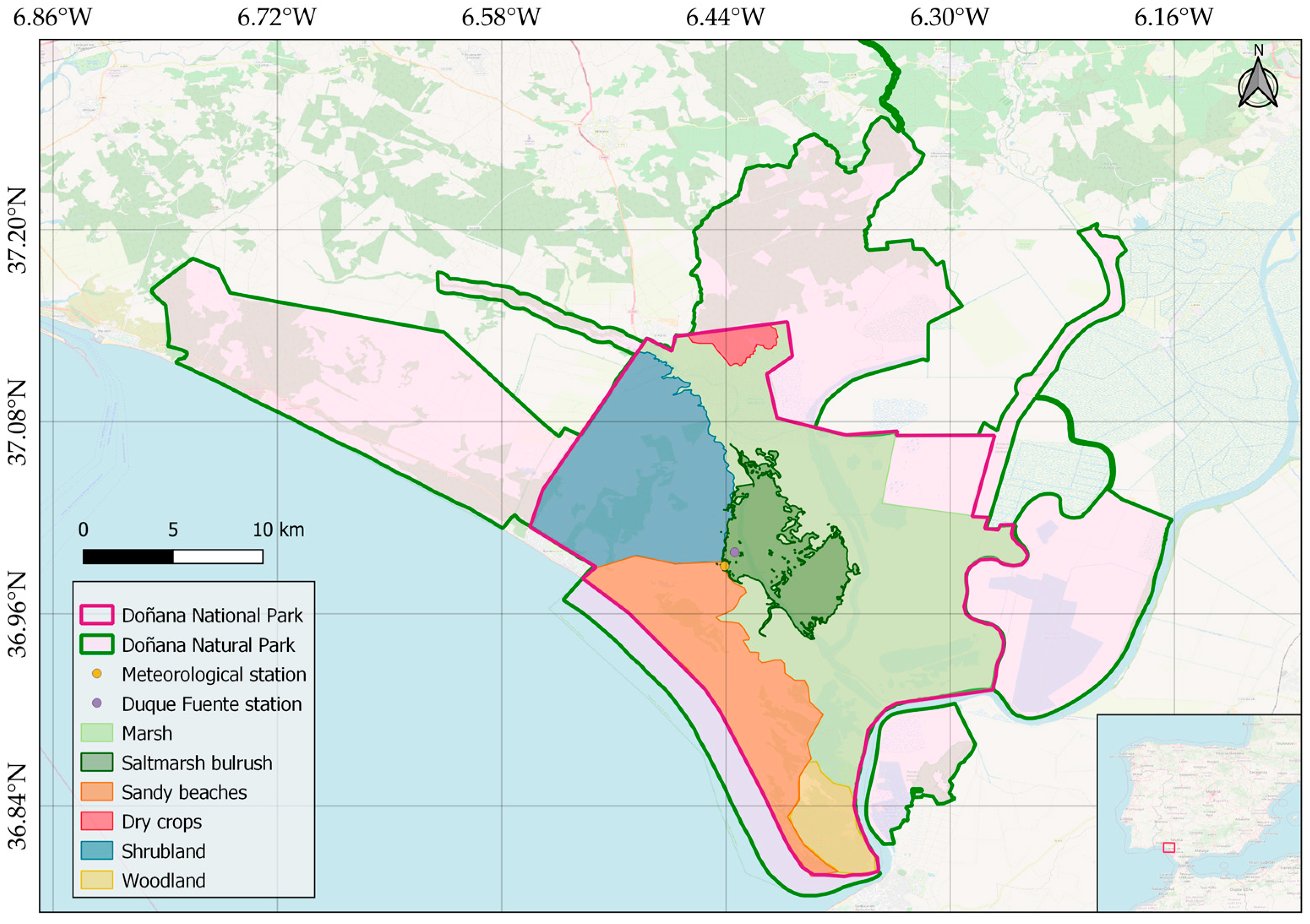
The workflow is implemented in a wetland ecosystem located in Doñana National Park, situated in southwest Spain (Figure 1). The Doñana National Park (DNP), with an extension of 537 km2, is a UNESCO Biosphere Reserve and a Natural Heritage and a Ramsar site [47]. It shelters the largest wetland in Western Europe, composed of a complex environment of marshlands and dune ponds (270 km2) enclosed by Mediterranean scrubland, pine forests, a dune ecosystem, and cultivated areas [48]. This study focuses on the areas dominated by saltmarsh bulrush (Bolboschoenus maritimus).
The wetlands of the Doñana National Park are essential for the conservation of biodiversity and the provision of ecosystem services [48,49,50]. Regardless of their importance, the area has experienced numberless threats associated with ecological disasters, both due to anthropogenic pressure [51,52] and exceptional weather conditions [53], diversion of water and overexploitation of groundwater for agricultural purposes, and land-use changes [48,54,55]. These activities have affected both the water quantity and quality available to the marsh and dune pond ecosystems [56,57]. Previous research predicted exacerbation of the problems due to climate change in the absence of better management of the water resources in the catchment and the aquifer [56]. The need for monitoring activities in the region is, therefore, crucial.

2.2. Data

Doñana’s Singular Scientific-Technical Infrastructure (ICTS-RBD) provided data access and support to carry out the study case at the Doñana Protected Areas. The in situ monitoring infrastructure operated by the ICTS-RBD consists of an eddy covariance tower, the “Duque Fuente flux tower“ and a meteorological station, named the “Palacio Doñana station”. The location of the station and tower is displayed in Figure 1.
The eddy covariance data set consisted of 30-min measurements of Net Ecosystem Exchange (NEE) and ancillary meteorological data collected between the 1st of October 2020 and the 8th of June 2021. The meteorological data set from “Palacio Doñana station” consisted of daily estimations of multiple environmental variables of the region including daily cumulative precipitation and average temperature collected between 1976 and 2021. Table 1 and Table 2 display the data and metadata available in the ICTS-RBD monitoring system.
To differentiate the night periods for the NEE data processing, the Global Radiation data set (SW_IN) was retrieved from the SARAH solar radiation data records provided by the EUMETSAT Climate Monitoring Satellite Application Facility (CM SAF). The SW_IN records were available for the years 2005 to 2016; therefore, we assumed that the global radiation data for 2020 and 2021 were equal to the daily average value of solar radiation for the years 2005 to 2016. Night periods were identified by using a threshold of 20 W m−2.
Meteorological precipitation data were additionally retrieved from a global data set to assess the capacity of these products to compute the study workflow and supply sites lacking daily measurements of meteorological variables. Daily measurements of precipitation were collected from the Climate Hazards Group InfraRed Precipitation with Station data (CHIRPS) database (https://www.chc.ucsb.edu/data/chirps, accessed on 12 December 2022) at the Duque Fuente tower location.
ICTS-RBD also provided the vegetation map of the wetlands of Doñana. The latest was used to qualitatively assess the results of the unsupervised classification to upscale the outputs of the model beyond the climatological footprint. The vegetation map was previously computed with supervised classification approaches for the year 2009 by the ICTS-RBD.

2.2.1. Remote Sensing Imagery

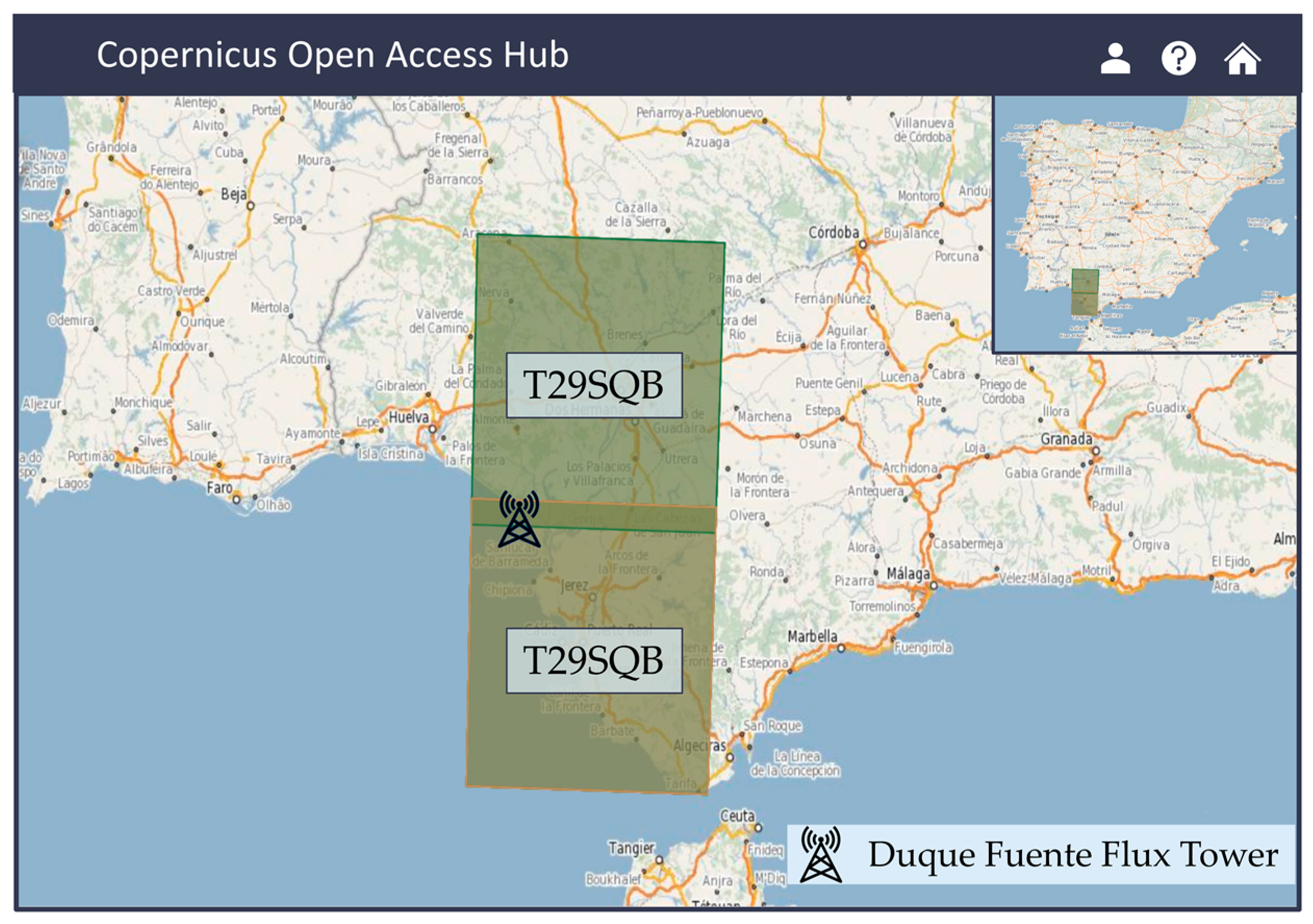
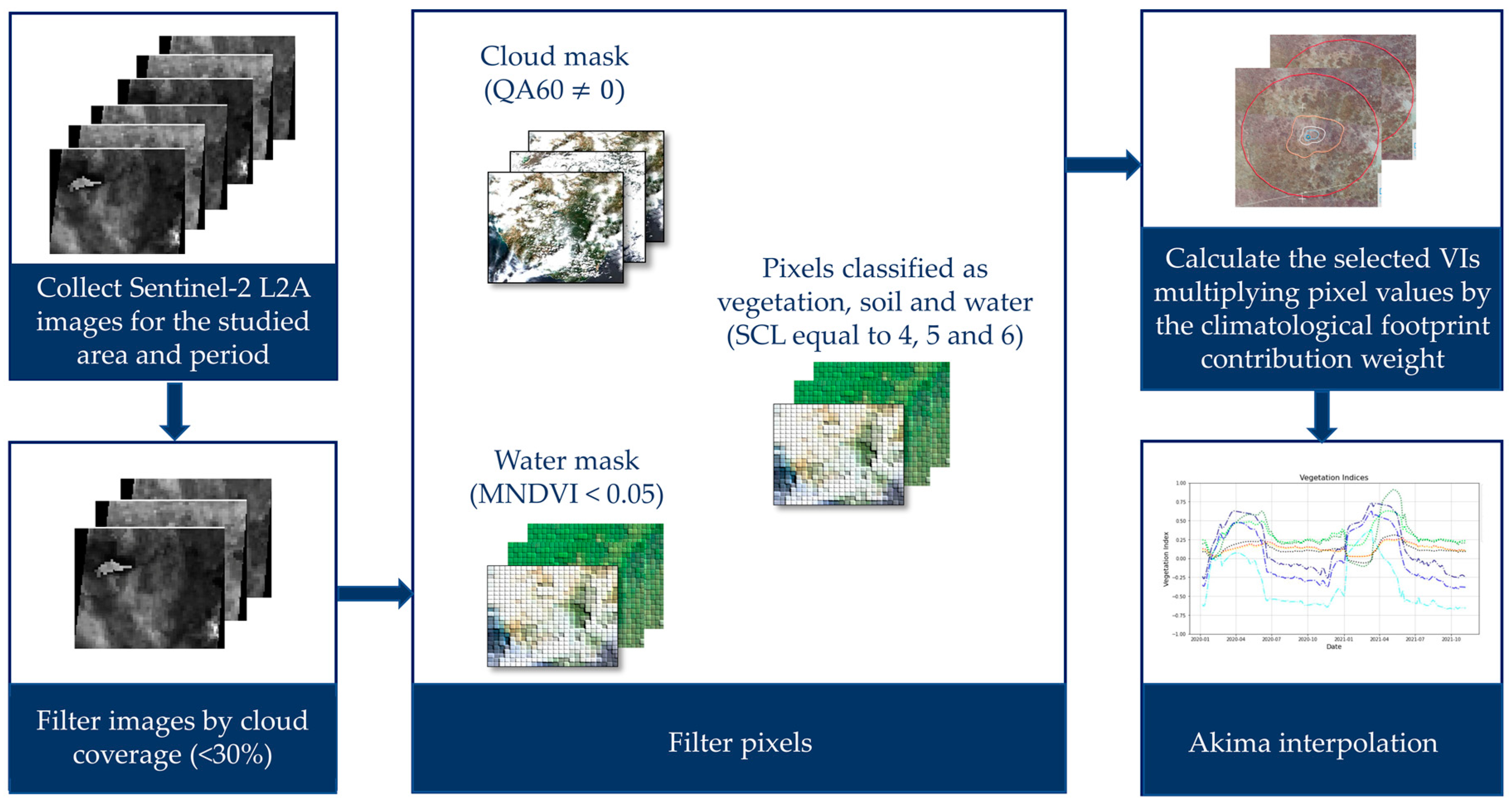
For this study, Level-2A Sentinel-2 (S2) products were used. Images were accessed through the Google Earth Engine (GEE) data catalog “COPERNICUS/S2_SR” by means of the python client “ee” package (https://gee-python-api.readthedocs.io/en/latest/ee.html, accessed on 12 December 2022). All images available in the region of interest were collected, and those correspond to the tiles T29SQA and T29SQB (Figure 2). Images with high cloud coverage were removed. The cloud coverage threshold was set at 30%. Specific treatment was applied afterward to remove remaining pixels with high cloud coverage and not belonging to vegetation (e.g., water bodies, snow, temporal floods, or another temporal phenomenon). The cloud mask was applied to the images using the Scene Classification Map (SCL) and the supplementary band QA60. The SCL allows for tracing or marking defective pixels whereas the QA60 band helps distinguish between opaque and cirrus clouds (https://sentinel.esa.int/web/sentinel/user-guides/sentinel-2-msi/processing-levels/level-2, accessed on 12 December 2022).
To remove flooded pixels, at first, we applied the water mask of the SCL on the images; however, the mask also covered and removed flooded regions with standing vegetation or biomass contributing to the GPP of the ecosystems. Previous research estimating PP through correlation with satellite-derived VI suggested removing the influence of water pixels at Doñana National Park by selecting a threshold corresponding to the baseline of the phenological curve [58]. Kordelas et al. [59] suggested the use of the Modified Normalized Difference Vegetation Index (MNDVI) to identify vegetation in the flooded area of Doñana National Park, which was preferred over the Normalized Difference Vegetation Index (NDVI) that created false positives in areas where vegetation was not expected. For this reason, we decided to filter the water pixels by defining a threshold of the MNDVI. A baseline of MNDVI = 0.1, corresponding to the minimum reflectance observed in the vegetation throughout the year was found. A threshold of 0.05 was then selected to identify and remove water pixels (MNDVI < 0.05) not contributing to the GPP of the ecosystem. Table 3 displays the number of images for each tile for different cloud coverage thresholds and months during the period of analysis. All available images from 1 October 2020 to 8 June 2021 with cloud coverage lower than 30% were used for the computation of the workflow.
Together with the Sentinel-2 images, MOD17 products were also retrieved from the GEE catalog for the same period (1 October 2020 to 8 June 2021). This data set was used to compare the Sentinel-2-based GPP results with the MOD17 products and analyze their performance in comparison with in situ measurements.

2.3. Methods

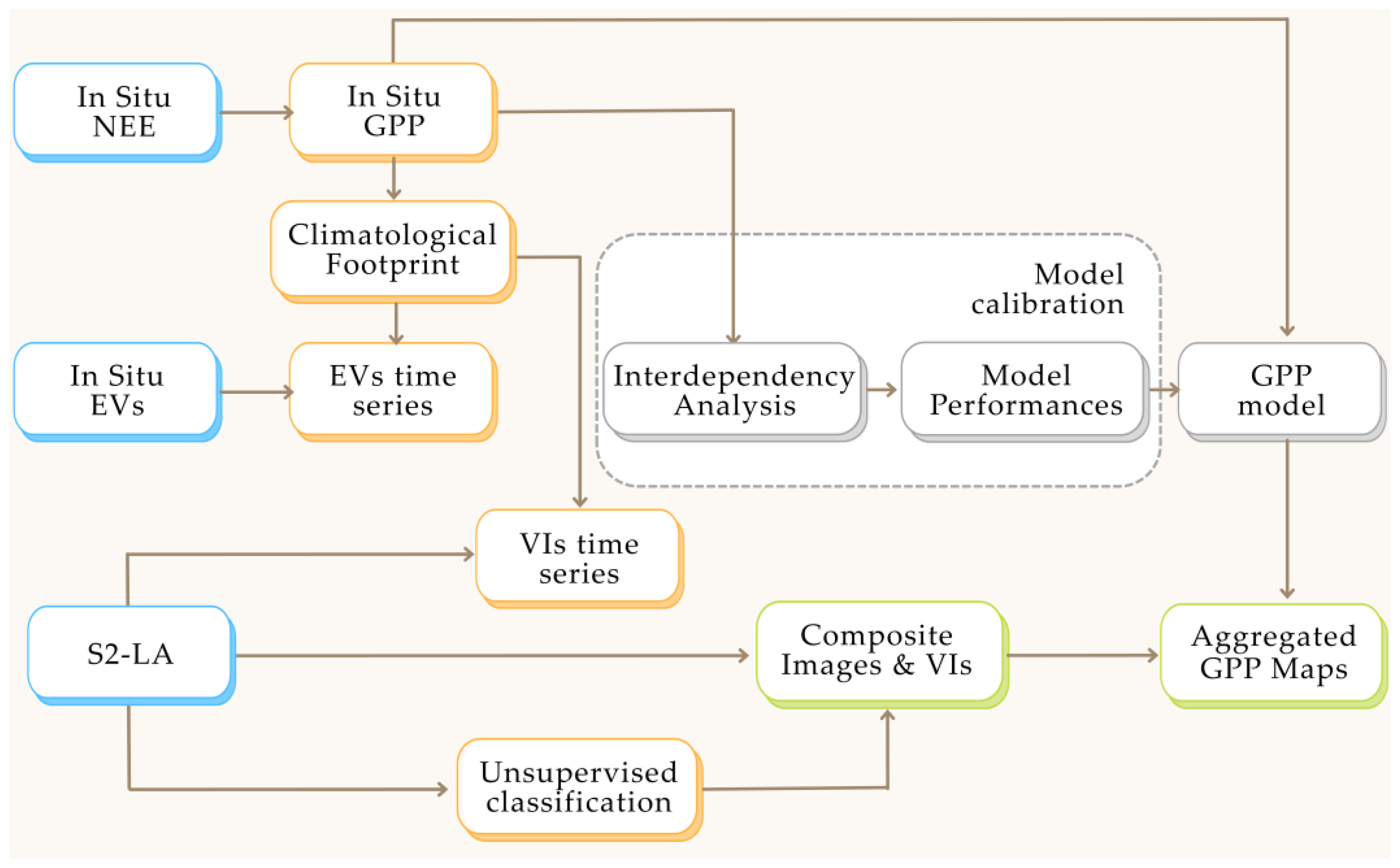
The research workflow is schematized in Figure 3. It consists of nine main processes: (1) derivation of in situ GPP daily measurements from NEE; (2) estimation of the climatological footprint; (3) computation of the VIs time series within the climatological footprint; (4) computation of time series of all the environmental/meteorological variables; (5) interdependency analysis between in situ GPP and the VIs-EVs and model formulation; (6) calibration and validation of the model; (7) unsupervised classification of the area to select an upscaling region; (8) computation of GPP maps. The details of each process are provided in the sections below.

2.3.1. In Situ Time Series of GPP

In situ measurements of NEE were used to derive the time series of GPP. NEE is measured at the Duque Fuente flux tower (Figure 1) by means of the Eddy Covariance (EC) technique, a method to ascertain the exchange rate of carbon dioxide rates in ecosystems [60]. We processed the 30-min NEE records following the standardized processing methodology proposed by Papale et al. [60] and using the ancillary meteorological data of the EC system. The methodology included four steps aiming at correcting the data and estimating the GPP: (1) outlier detection, (2) velocity friction filtering, (3) carbon fluxes partitioning to derive GPP, and (4) gap filling using ancillary environmental data. The estimates were finally aggregated to derive daily values of GPP (in gC m−2 day−1) used in the model calibration and validation. For a detailed description of the steps, refer to the paper by Papale et al. [60].
The aforementioned process was implemented through the hesseflux Python package [61] adapted to process the European Fluxes Database Cluster (EFDC) format files (http://www.europe-fluxdata.eu/, accessed on 12 December 2022). Full documentation of the hesseflux package is available at https://mcuntz.github.io/hesseflux/, (accessed on 12 December 2022). In the context of the study case, we adopted a velocity friction filtering threshold of 0.14, as previously conducted for salt marshes [62], since the threshold could not be automatically computed because of the lack of full-year measurements.

2.3.2. Climatological Footprint

To better interpret flux tower measurements, flux footprint models have been used to estimate the size and position of the surface area contributing to the measured flux [63]. The knowledge of this area, also known as flux footprint, is of extreme importance in upscaling the model from a single site flux measurement to an ecosystem or regional scale. Wind and turbulence conditions, and atmospheric conditions and surface characteristics contribute to the flux measured at a specific point in time. To estimate the flux footprint, we used the Flux Footprint Prediction (FFP) model of Kljun et al. [63] available in Python code (https://geography.swansea.ac.uk/nkljun/ffp/www/, accessed on 12 December 2022). We derived two aggregated footprints, also known as footprint climatology, three months of half-hourly input data for 2020 (October to December 2020), and six months of half-hourly input data for 2021 (January to July 2021).
Most of the input variables required for the FFP model were collected as a part of the EC system at the Duque Fuente flux tower. The variables included mean wind speed, measurement height above displacement height, equal to the anemometer sensor height minus the displacement height (3.75 m), the Obukhov length, the standard deviation of lateral velocity fluctuations and the friction velocity. The boundary layer height was estimated with the expressions described by Kljun et al. [63] for atmospheric near-neutral and stable conditions and here reported for completeness (Equation (1))
h = L 3.8 1 + 1 + 2.28 u f L 0.5 ,
where L is the Obukhov length, u* is the friction velocity and f is the Coriolis parameter calculated using the site’s latitude. The boundary layer is set to be at 1500 m at convective conditions defined as records in the eddy covariance data set when Obukhov length < 10 m [64]. The FFP model was computed to derive 20%, 40%, 60%, and 80% isolines. The 100% was not calculated with the FFP model but set as the fetch of the Duque Fuente tower according to the 1:100 displacement height-fetch ratio [65]. The derived footprints can be seen in Figure 4. The climatological footprints did not differ significantly in shape and size, having a surface of 5.72 and 5.30 ha within the 80% contour lines for 2020 and 2021, respectively.

2.3.3. Time Series of Vegetation Index

The filtered and masked Sentinel-2 images were post-processed to calculate multiple VIs. Table 1 lists the VIs employed in this research together with their equations. In total eight VIs were computed per image and selected based on a literature review of GPP modeling for different ecosystem types (Table A1). Those VIs can be divided into two major classes, (i) greenness-sensitive VIs ((Normalized Difference Vegetation Index (NDVI), Enhanced Vegetation Index (EVI), Two-bands Enhanced Vegetation Index (EVI-2), Red-edge Index (CLr), Modified Normalized Difference Vegetation Index (MNDVI)), and (b) water-sensitive VIs (the Modified Normalized Difference Water Index (MNDWI), Land Surface Water Index (LSWI), and Normalized Difference Infrared Index (NDII)). At first, we calculated the VI for each region within the climatological footprint, then we averaged them by a scaling factor. Finally, the total VI was computed as the sum of the VIs (Equation (2)):
V I = j = 1 k w j × i = 1 n V I i ,
where i is the number of pixels, j is the number of regions and w j is the weight of the j region calculated as (Equation (3)):
w j = O C L j ICL j n i
OCLCL j and ICLCL j being the outside and inner contour lines of the region j, respectively. With our approach, the weight is a constant value per region. This is a simplification of Cai et al.’s approach [25] that reduces the computational time of the calculation of the VIs. For our study, we computed five regions within the climatological footprint, each of them accounting for 20% of the NEE measured at the Duque Fuente flux tower. Finally, we used the Akima [66] fitting algorithms to obtain a continuous time series. Fitting algorithms were not implemented as we addressed the noise in the time series through the filtering and masking processes of the satellite images. Figure 5 summarizes the processing chain applied on the Sentinel-2 images to obtain the VIs time series (pre-processing steps have been described in Section 2.2.1).

2.3.4. Environmental Variables

PP is driven by several environmental drivers [36], and our model formulation also integrates different EVs. In this research we integrated the Air Temperature (AT), the Vapour Pressure Deficit (VPD) both retrieved from the EC tower and the temperature data provided by the meteorological station of the Doñana National Park (see Table 4). Those EVs were smoothed with a 7-day moving average window to reduce the noise in the time series.
Additionally, we integrated precipitation data from in situ measurements and from the CHIRPS data set as a proxy for the ecosystem water availability. Water stress, has been indeed identified as one of the main limiting environmental conditions of PP [8,67]. Particularly for the studied areas, the water availability is mainly regulated by rainfall events [58,68,69]. Precipitation, however, was not expected to have an immediate impact on the PP but rather the water accumulated in the system. Therefore, to account for the long-term soil moisture repletion process, we shifted the rainfall time series in time delaying the precipitation. Different time lags were considered. Moreover, the rainfall data were smoothed with a multiple moving average window to reduce the noise in the time series. Table 4 displays the environmental variables used in the study.

2.3.5. Interdependence Analysis and Model Calibration

An analysis of interdependence was performed to assess the correlation between the calculated in situ GPP and the set of all the possible combinations of VI × EV. The squared Pearson correlation coefficient (r2) was used to identify the product (VI × EV) with the highest correlation selected for the final model formulation. The latest followed the linear formulation suggested by Schubert et al. [45] and used by Cai et al. [25] reported in Equation (4):
G P P = m × ( V I × E V ) + b
where m and b are slope and intercept parameters, respectively, of the linear regression model. The Ordinary Least Squares (OLS) method was used to compute the parameters of the regression model. The OLS method is a statistical analysis aiming at deriving the m and b parameters of a linear model by minimizing the sum of squared errors, where the errors are the differences between the observed and predicted dependent variables. The m and b linear regression parameters were calculated using the OSL method with the following expressions (Equations (5) and (6)):
m = n x y x y n x 2 x 2
b = n x 2 y x x y n x 2 x 2
where y is the independent variable (GPP), x is the dependent variable (VI × E), and n is the number of data pairs. The estimation of the parameters was performed with a data set consisting of 80% of the original samples of in situ GPP. The statistical significance of the linear parameters and the overall model was evaluated with a confidence level of 95% (p-value < 0.05). In the case statistical significance was achieved, the model was accepted and used in the validation process.

2.3.6. Model Validation

The model was validated with an independent data set corresponding to 20% of the data. The validation data set was used to generate GPP predictions ( G P P p r e d i c t e d ). The predictions were compared with the flux-derived GPP ( G P P o b s e r v a t i o n ). The performances of the model were estimated in terms of Mean Absolute Error (MAE) (Equation (7)), Root Mean Squared Error (RMSE) (Equation (8)) and relative standard error of the estimates (Sest) (Equation (9)). The coefficient of determination (R2) between predicted and measured GPP was also calculated to evaluate to which extent the model explains the variance of the GPP.
M A E = G P P p r e d i c t e d G P P o b s e r v a t i o n n
R M S E = G P P p r e d i c t e d G P P o b s e r v a t i o n 2 n
S e s t = G P P p r e d i c t e d G P P o b s e r v a t i o n 2 n 2 G P P o b s e r v a t i o n n
where G P P o b s e r v a t i o n is the in situ GPP retrieved from the eddy covariance measurements, G P P p r e d i c t e d is the GPP derived with the empirical formulation, and n is the number of observations in the validation data set.

2.3.7. Vegetation Classification Maps

In order to observe the spatial pattern of GPP, the model was upscaled to the surrounding areas of the eddy covariance tower. An unsupervised classification algorithm was used to identify regions with the same land cover (reflectance properties) as those identified within the flux footprint. The identified regions were assumed to have homogeneous vegetation with similar biophysical properties, photosynthesis activity and GPP seasonality of those within the footprint. The unsupervised classification was performed on a composite image created by using all the Sentinel-2 images available for the study period preprocessed as described in Section 2.2.1. The k-means clustering algorithm developed by Arthur and Vassilvitskii [70] was used to perform the unsupervised classification and implemented through the Clusterer.wekaKMeans method of the “ee” package in python. The algorithm minimizes the average squared distance between the points in the same cluster. The use of this robust unsupervised clustering method helps overcome the need for expert human knowledge required for supervised classification and has already been used in similar studies [71,72,73]. Our area of study was classified into seven classes using 5000 training pixels with a scale of 10 m retrieved from the study area

2.3.8. GPP Maps with Composite Images

Once the vegetation classification map was obtained, the model was applied to the regions having the same land cover of the area within the climatological footprint. By doing so, we produced GPP maps for each Sentinel-2 available image. Then, we aggregated the obtained maps to produce an estimate of the monthly/annual GPP. The latest is indeed a highly important product relevant for further analysis of the ecosystem’s status. Annual maps of GPP are useful for trend analysis, the identification of the degradation of the ecosystem functions, and for computing annual NPP if knowledge of the autotrophic respiration processes of the ecosystem is known [35,36].
To create an operational monitoring tool easy to be implemented by stakeholders and policymakers that bypasses the limitations of cloudy satellite data, we propose a simplified model for the calculation of GPP for a specified time window. Aggregated products of GPP are computed as (Equation (10)):
G P P = i = 1 n G P P i = i = 1 n m × V I i × E V i + b
where n is the number of days within the time window, and m and b are the model parameters, and therefore, constant. Assuming that the VI is constant within the selected time window ( V I i = V I ), Equation (10) can be written as:
G P P = m × V I i i = 1 n E V i + b × n
The model formulation (Equation (11)) is susceptible to high deviation if the assumption cannot be guaranteed. In this research we propose to work with a 30-day time window; however, we also applied a 15-day time window to compare the benefits of increasing the frequency of the map generation.
The GPP products are finally aggregated to derive a GPP map for the full period of analysis.

3. Results

3.1. Interdependency Analysis and Model Calibration

The interdependency analysis between the in situ GPP and VIs showed that greenness-sensitive VIs derived the highest coefficients of determination. The CLr resulted in the highest correlation with GPP, with a coefficient of determination R2 = 0.90 and statistical significance p < 0.05. The NDVI showed the lowest correlation among the greenness-related VIs with R2 = 0.57. Water-sensitive vegetation indices did not show a high correlation with the GPP measurements. Among those, the NDII had the highest R2 of 0.39 and a significance level of p < 0.05. Table 5 summarizes the results of the interdependency analysis, obtained using only SRS VIs.
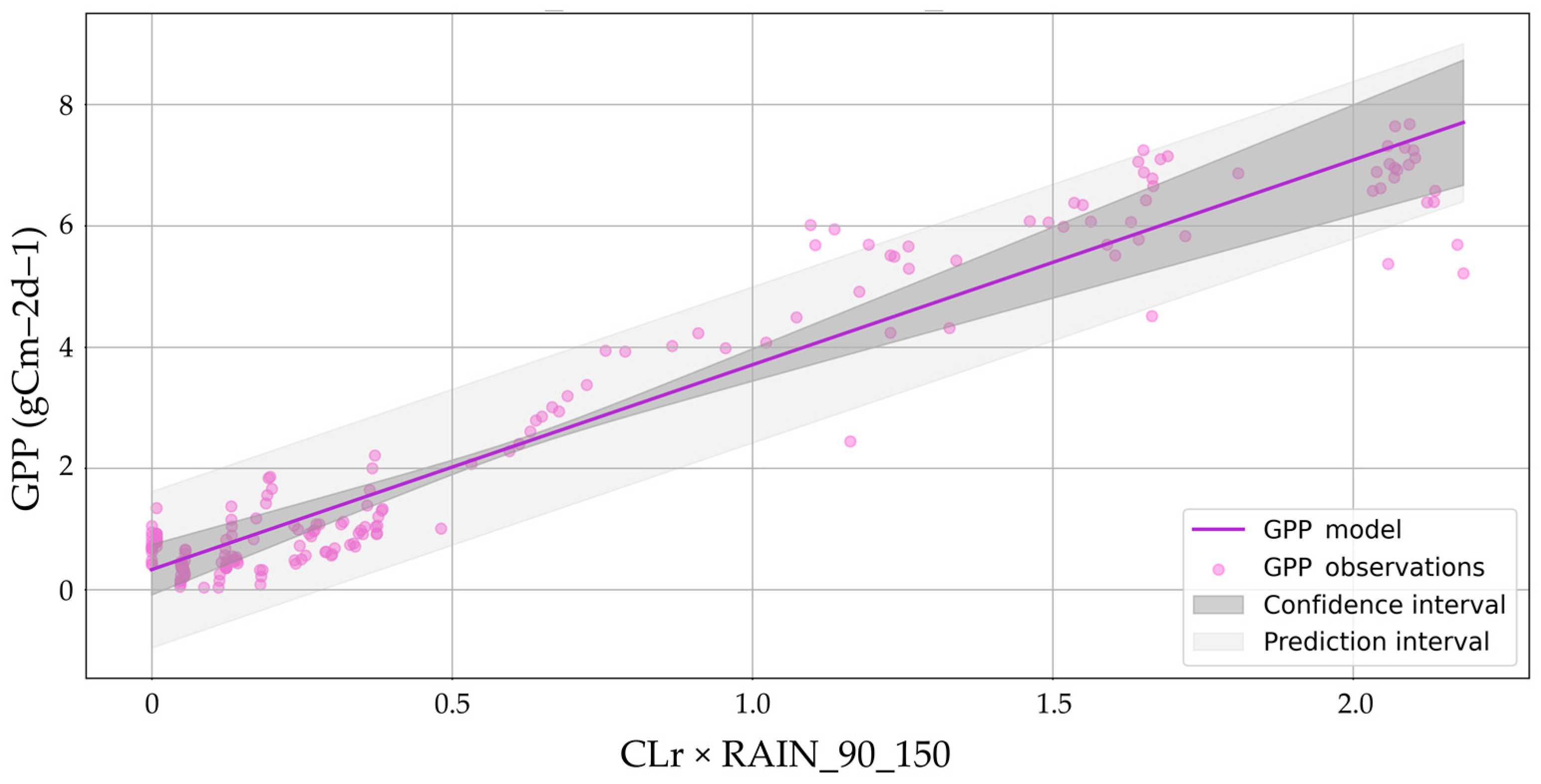
By including the EV in the model formulation, we observed an increase in the correlation with in situ GPP. In total 784 models (VI × EV) were analyzed and the coefficient of determination was acquired for all the models. In general, the VIs showed a higher correlation when combined with rainfall-related variables in contrast with temperature or vapor pressure deficit data. The first fifty VIs and environmental variables combinations with higher correlation are displayed in Table A2. The product between the CLr and the rainfall data calculated with a rolling average of 90 days and delay of five months (RAIN_90_150) yielded the strongest correlation with an R2 of 0.93. We, therefore, selected the CLr and the RAIN_90_150 for the model formulation (Equation (12)):
G P P = m C L r × R A I N _ 90 _ 150 + b
where m and b represent the slope and intercept parameters of the linear model, estimated by means of the OLS method. The summary of the calibration process, including the parameter values and their corresponding significance levels, is displayed in Table 6.
From the calibration process, an offset parameter b = 0.3308 and a scale parameter m = 3.3743 were derived. The final linear model for GPP prediction was, therefore, formulated as follows:
G P P m o d e l = 3.3743 C L r × R A I N _ 90 _ 150 + 0.3308
The scatter plot between the observed GPP values and the estimated ones is shown in Figure 6 together with the 95% confidence interval. It can be seen that the model performances were accurate with most of the points within the prediction interval.

3.2. Model Validation

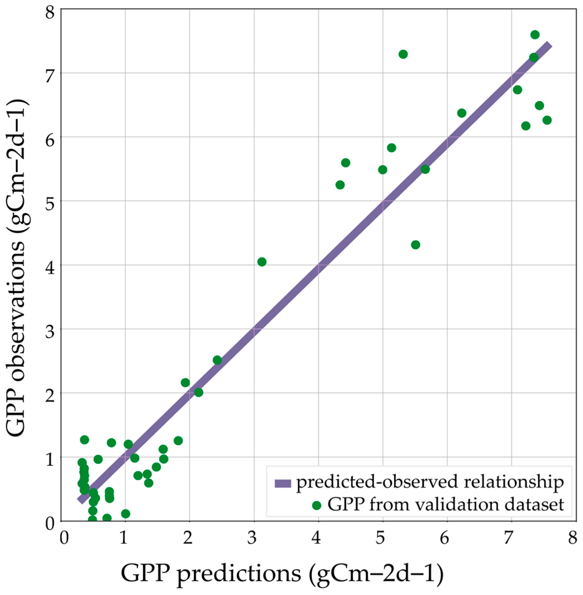
The calibrated model was used to predict GPP ( G P P p r e d i c t e d ). The results were compared with an independent validation data set corresponding to 20% of the original GPP sample ( G P P o b s e r v e d ). The model resulted in an MAE of 0.52 gC m−2 d−1, RMSE of 0.63 gC m−2 d−1 and Sest equal to 0.27. The latest indicated that the model predictions had a standard deviation of 27% with respect to the GPP observations.
The scatterplots of observed versus estimated values of GPP for the validation phase (Figure 7) show that the slope of the predicted-observed relationship did not differ significantly from 1 (0.97), indicating that the model predictions neither under nor overestimated the observed values of GPP.

3.2.1. Comparison with MOD17 Products

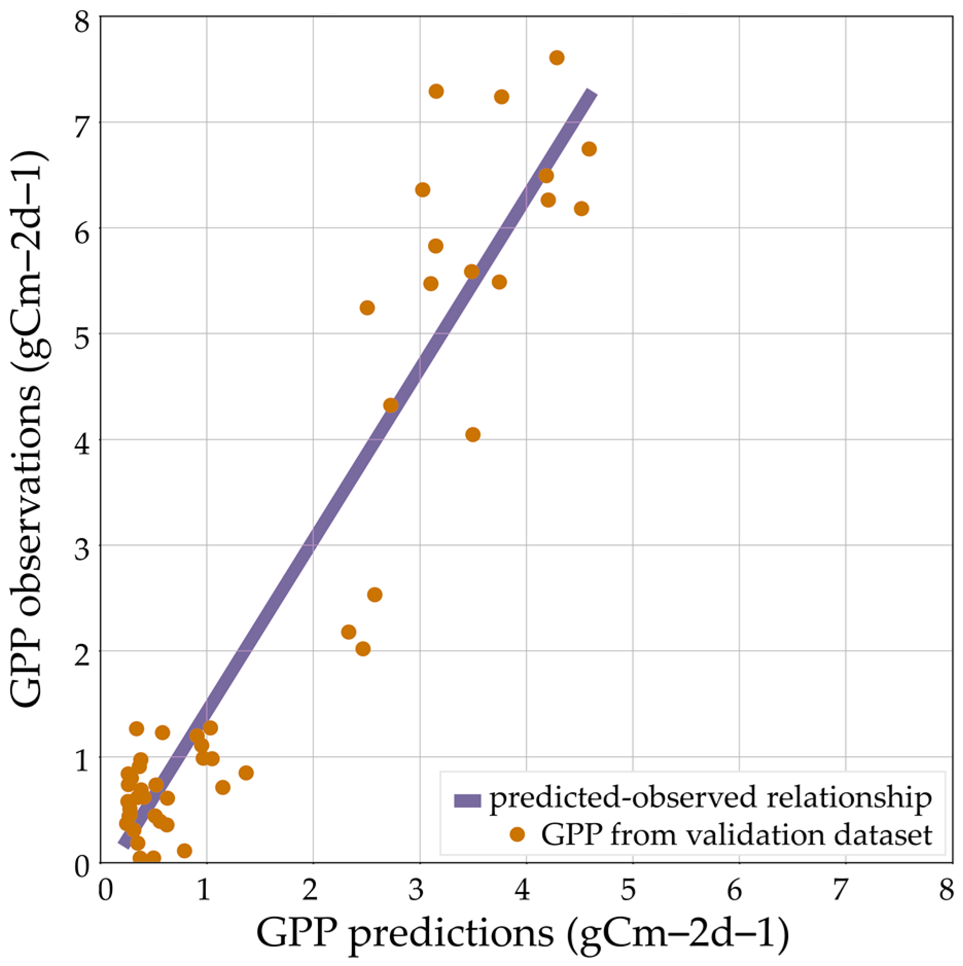
To evaluate our model performance in comparison with existing satellite-based products, we produced time series of MOD17. At first, we compared in situ GPP and the MOD17 1 km 8-day GPP products. From the scatter plot in Figure 8, we can observe that the slope of the predicted-observed relationship of the MOD17 product is higher than 1 (1.62) indicating that the MODIS model is underestimating the ground GPP.
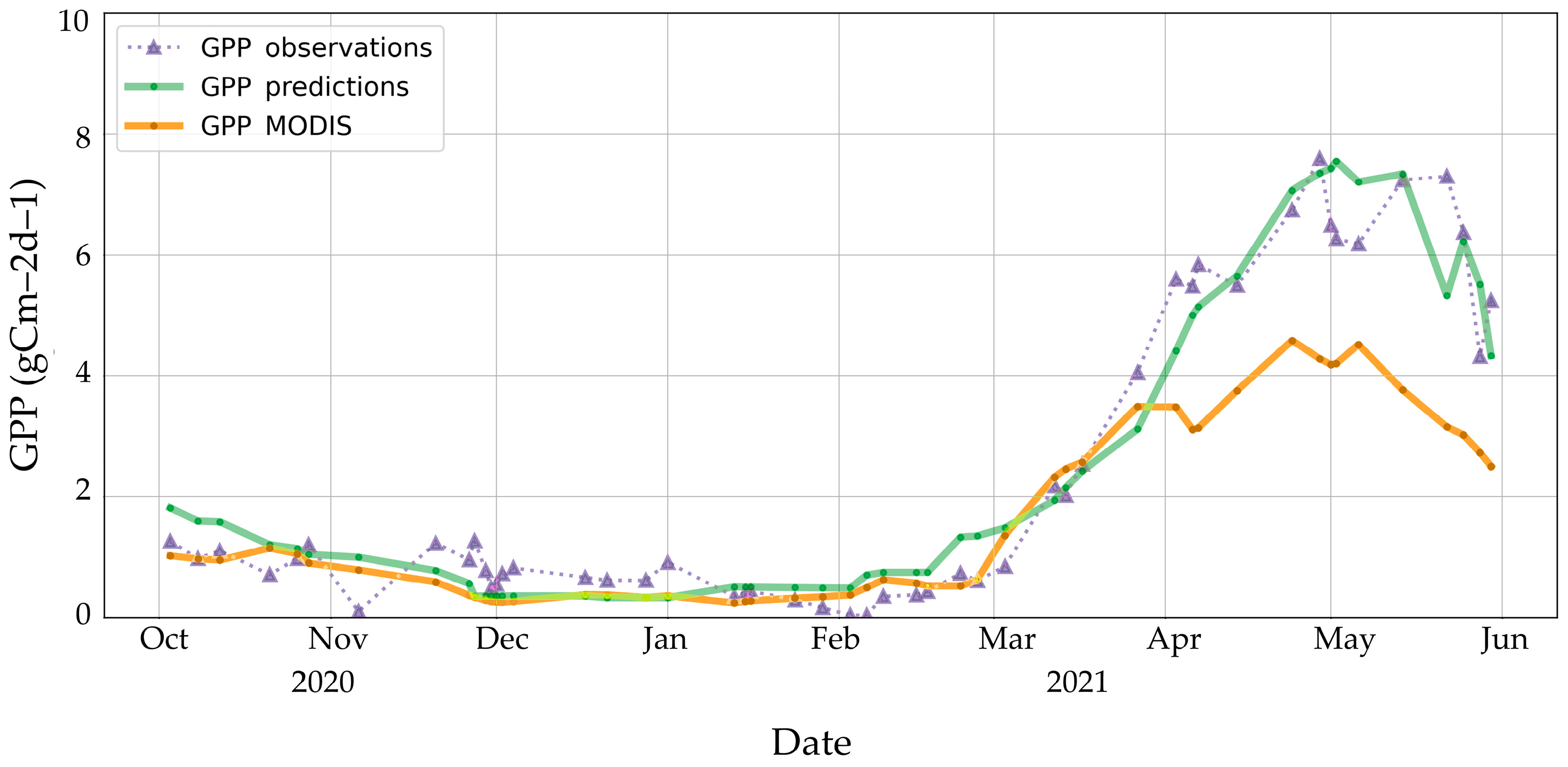
Then, we compared both our model and the MOD17-based time series with in situ measurements of GPP. Both the MOD17 and our GPP products showed a general agreement with the observed data, especially during the fall and winter months when low primary productivity was observed (October 2020 to February 2020). For the months with a peak of GPP (April 2021 to June 2021), our simulated GPP performed better than the MOD17 product, which was underestimating the observed GPP measurements (Figure 9).
A comparison of the two models in terms of MAE, RMSE, and Sest is presented in Table 7. While having a high correlation with flux-derived GPP, the MOD17 products presented higher prediction standard errors due to the high underestimation of the GPP during the peak biomass suggesting that the calibration of the MOD17 products should be performed together with the investigation of the sampling procedure that can ensure that collected ground measurements are adequately representative and sufficient to validate the target low resolution EO product.

3.2.2. Vegetation Maps

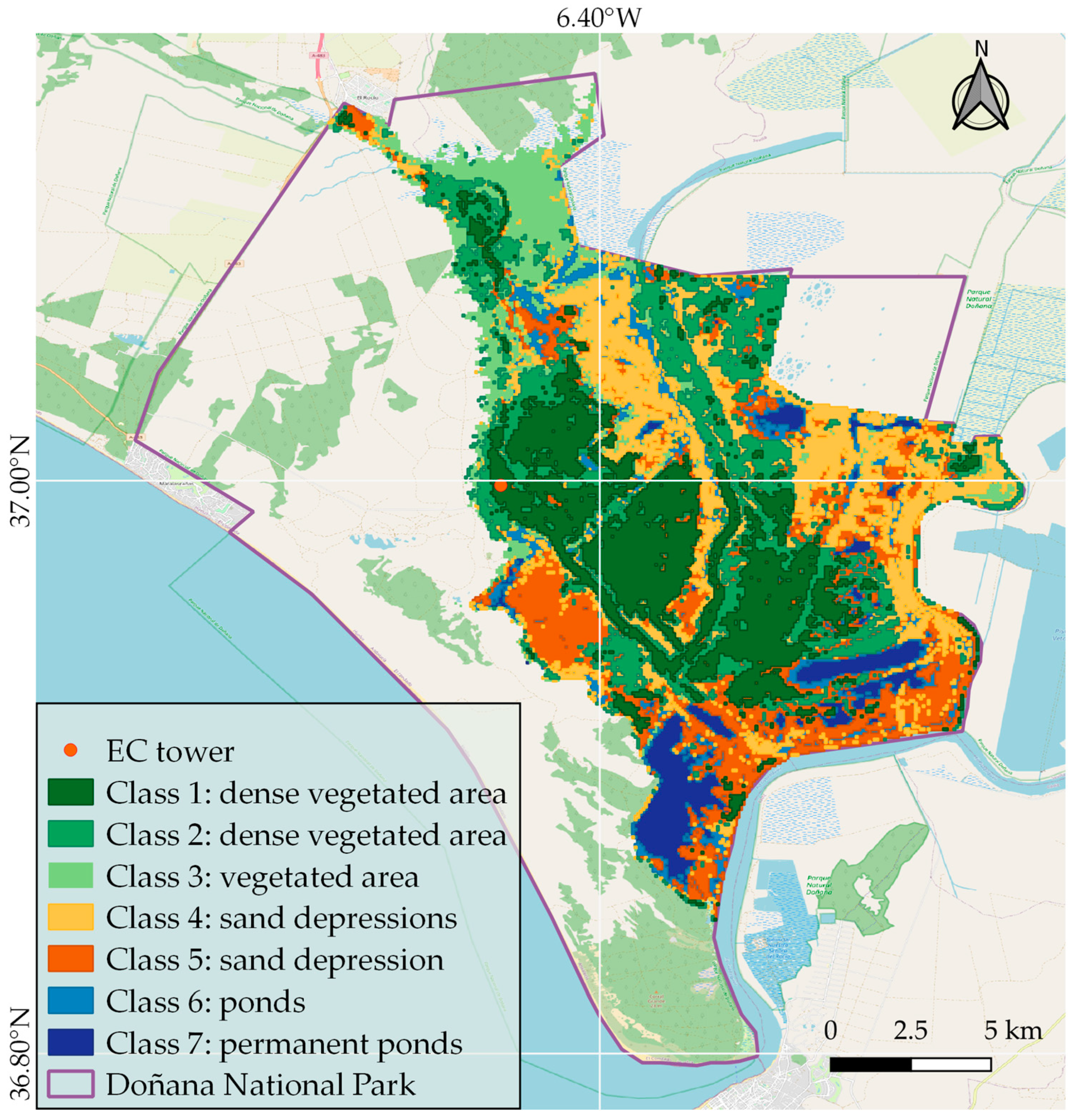
The unsupervised classification of the wetlands of Doñana National Park derived seven classes displayed in Figure 10. Classes can be grouped into (i) vegetated areas (green areas); (ii) sand depression areas (yellow and orange areas) and (iii) flooded areas (blue areas). Visual comparison of the outcomes with different land cover classification maps of the region [48,58,74,75] showed good performances of the unsupervised classification algorithm. The flux tower is located within the green zone (dense biomass area) and measures carbon fluxes from the densely vegetated areas on the west side of the wetlands (see Figure 10).
By a visual comparison with the vegetation classification map of 2009 provided by ICTS-RBD (Figure 11), we could see that those green areas correspond to the regions dominated by Bolboschoenus maritimus vegetation, commonly named saltmarsh bulrush. The vegetated-marsh area of the Doñana National Park was also identified in 2017 by Lumberries et al. [58] (highlighted with the red line in Figure 11). Being one of the most recent classifications we could find in literature, we decided to adapt our model to the same region identified by Lumbierres et al. [58]. This area dominates the region surrounding the eddy covariance tower and has similar biomass production.

3.2.3. GPP Maps with Composite Images

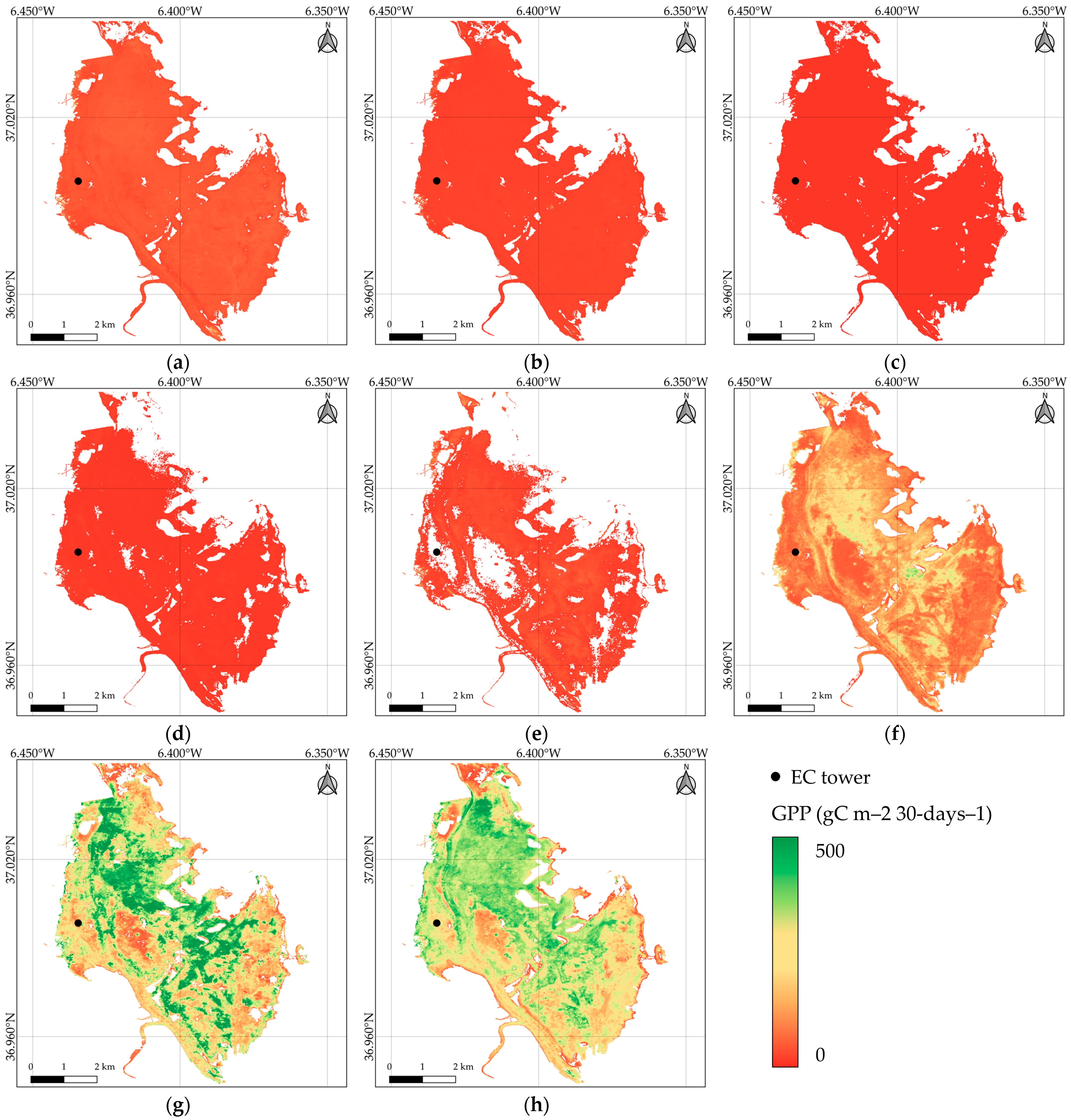
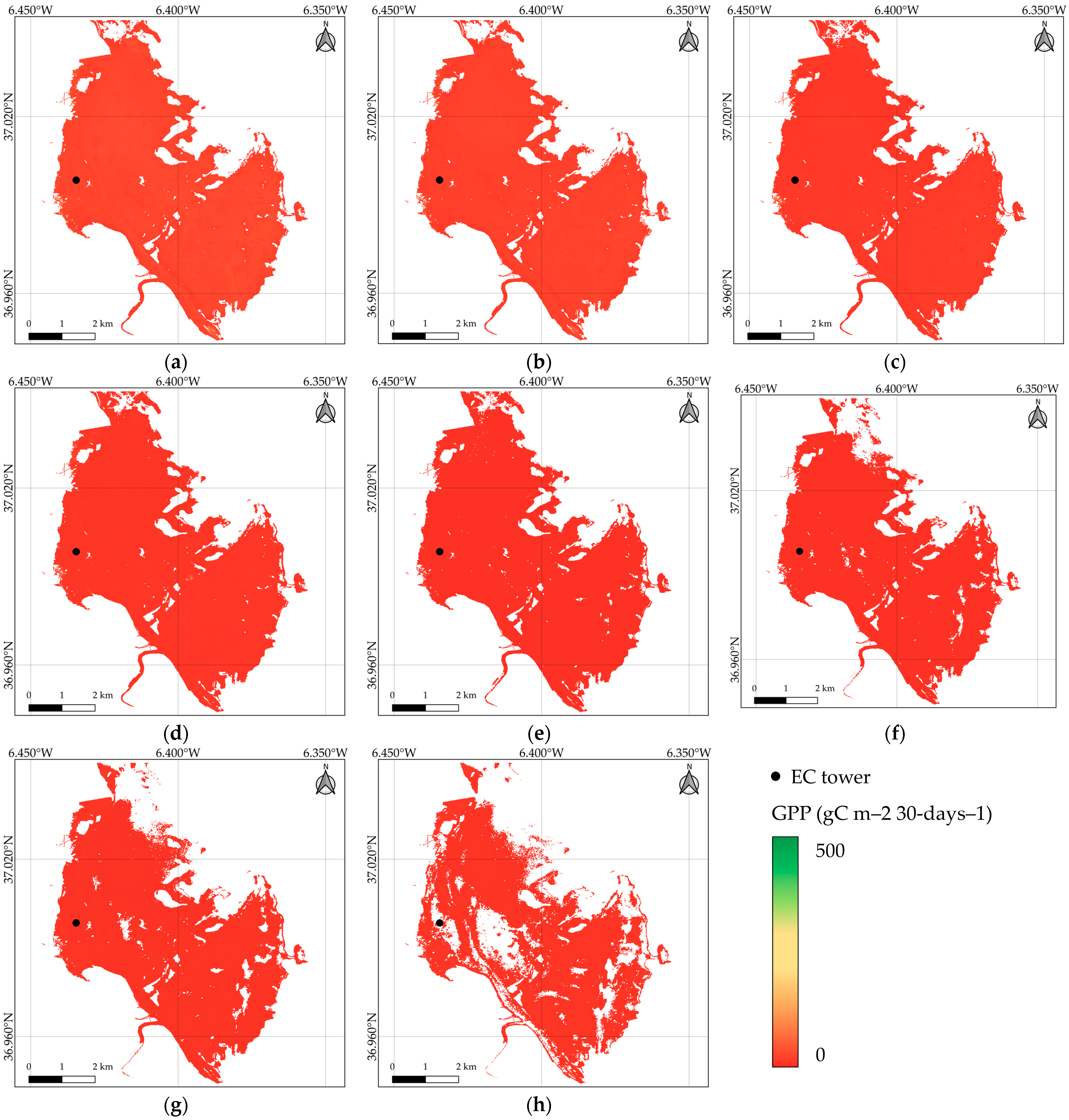
The following figures display the monthly maps of GPP derived with composite images per month (Figure 12). The model well represented the interannual variability and trend of GPP over the study area. GPP is low during the start of the fall and winter months (October–January). At the end of the wet season, when the water availability in the ecosystem is at its maximum [58], the GPP content increases and reaches its maximum during the springtime (April–May). More spatial and temporal details of the variation of GPP can be seen in Figure A1 where a comparison between the Sentinel-2 and MOD17-derived products obtained using a monthly composite image is presented.
The model accuracy in the selected area could not be directly assessed given the lack of in situ measurements outside the climatological footprint. Attempting to quantify the goodness of the model, we compared the predicted GPP within the footprint with the monthly carbon flux measured at the Duque Fuente flux tower (Table 8).
From Table 8, we observed that the model generally overestimates the ground measurements of GPP which varies within a range of ±13 gC m−2 month−1 in comparison to the in situ measurements. A MAE equal to 9.97 gC m−2 month−1, RMSE equal to 14.64 gC m−2 month−1, and a Sest of 0.24 are found.
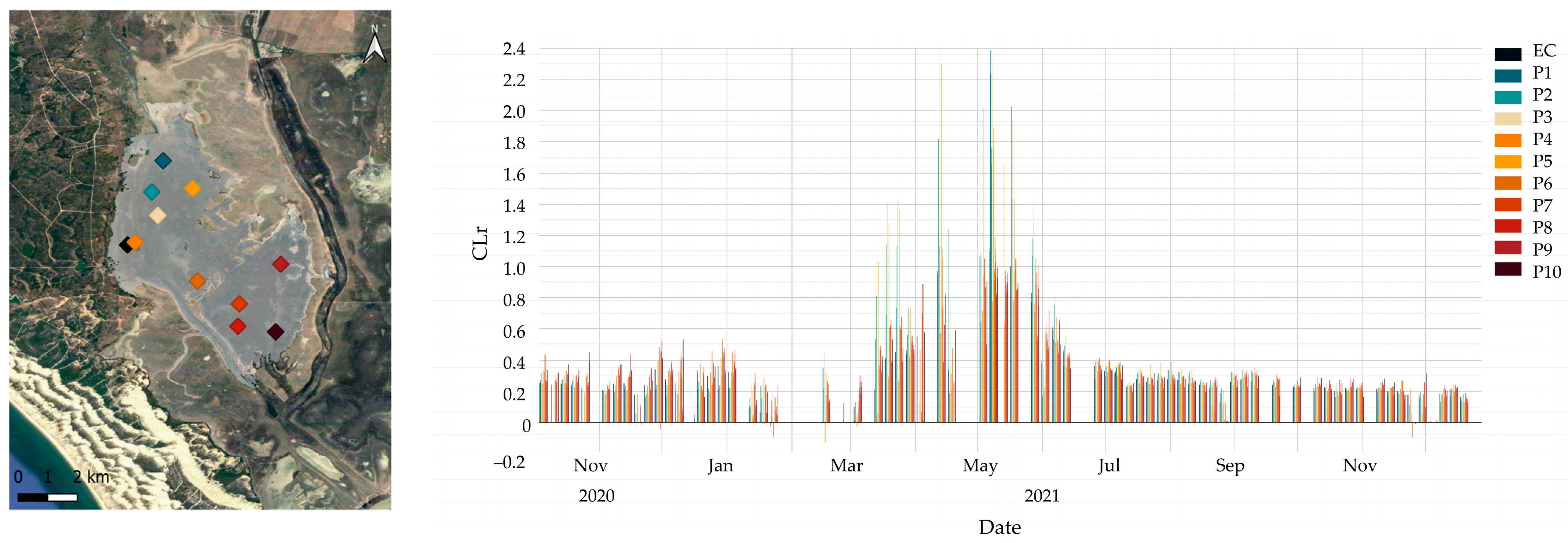
To improve the estimations of the GPP, we decided to reduce the time window and produce 15-day maps. Reducing the time window allows indeed for a better discretization in time and particularly accounts for the high variation of the CLr index during the spring. Equation (11) assumes that the VI is constant during the months and with high variation of CLr, the GPP can be over or underestimated. The time series of CLr for different pixels within the studied area is shown in Figure 13. GPP maps were, therefore, retrieved for the entire period using a 15-days composite image. The resulting maps are displayed in the figures below (Figure 14 and Figure 15).
The production of maps using 15-day composite images was affected by the high cloud coverage over the study area. This phenomenon can be clearly observed in the maps produced for the second half of February and April 2021. This hampered the estimation of GPP for the considered time range. The 15-day composite image, however, also allowed for better identification of the flooded period. This was the case for the month of January 2021. Comparing the first and second half of the month, we can observe that some pixels were left out in the second half of the month. Those corresponded to a phase of high flood and thus pixels were masked and GPP set to zero in the flooded regions.
Table 9 shows the comparison between the 15-day GPP predictions and the ground measurements of GPP. We observed that the model performances slightly improved compared to the monthly prediction, confirming that a smaller time window could improve the estimation of GPP.
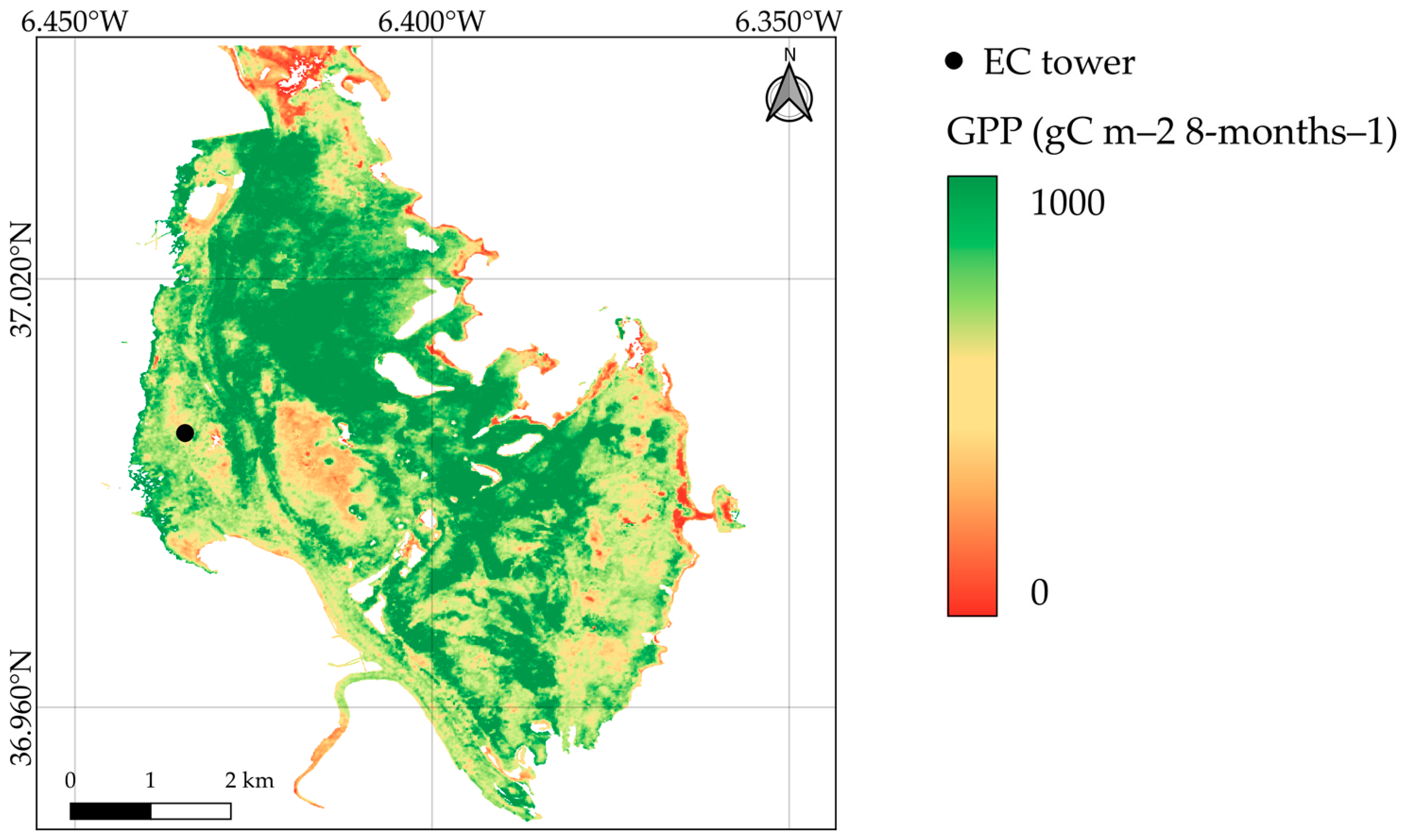
Finally, a GPP map was produced for the entire period of study (Figure 16). An average GPP of 770.20 gC m−2 (8 months)−1 was found. This value is comparable with reported GPP values [58].
When compared to in situ measurements at the Duque Fuente station, a MAE equal to 9.68 gC m−2 month−1, an RMSE equal to 13.81 gC m−2 month−1, and a Sest of 0.23 were derived.

4. Discussion

The development and application of a workflow to derive an empirical model of gross primary productivity from remote sensing imagery have been demonstrated at Doñana National Park wetlands. The model has been upscaled for the estimation of GPP in the marsh area surrounding the EC tower. The generated monthly maps of GPP have the potential to provide detailed information on the patterns and dynamics of primary production.
The model selection led to a linear regression model driven by the remote sensing based red-edge chlorophyll index CLr in combination with the rainfall data. This confirmed previous research outcomes on the sensitivity of the red-edge to canopy biomass, chlorophyll content and photosynthesis activity [76,77,78] and thus on the enhanced estimation of the vegetation biophysical characteristics [33,79,80]. In general, analyzing each VI proposed in the methodology, we observed that the greenness-sensitive VIs performed the best. Narrowband greenness VIs also showed good performances. The EVI and EVI-2 resulted to be more sensitive than NDVI, confirming that EVI can improve the estimation of productivity in areas with dense vegetation being less prone than NDVI to noise caused by soil and atmospheric effects [81,82]. Water-sensitive VIs, such as the LSWI and the MNDWI, did not show a high correlation with in situ GPP. Previous researchers have shown that these indexes are more sensitive to drought [34,83] than greenness-sensitive VIs and thus we suggest further investigation of their performances during dry phases and in ecosystems undergoing seasonal droughts.
The integration of satellite-derived VIs with environmental variables in the model formulation increased the correlation with in situ GPP. Particularly, rainfall data increased the model performances confirming that the biomass production of the Doñana marsh ecosystem is strongly dependent on precipitation [58]. As a result of the high exploitation of water resources in the proximities of the Doñana National Park, the current flooding regime of the natural marsh is mainly determined by local precipitation [16]. The wetlands’ size and depth change remarkably between years, driven mainly by the variability in the precipitation [48], indicating that the flood levels and associated primary productivity in the ecosystems also correlate with the precipitation regimen. The association has also been supported by other authors studying species distribution stating that precipitation is the main driver of primary productivity and associated support of habitats for waterbirds in the ecosystem [84].
The phenological cycle of the vegetation of the study area is also well reproduced, confirming the choice of our model predictors. [48,58] report that the biomass and associated photosynthesis activity observed through the total intake of carbon dioxide or GPP is low during the start of the rain season (October–December) and the initial stage of the more intense precipitation and flood season (January–February). Then, the GPP content increases in the middle of the wet season when the water availability in the ecosystem reaches a maximum (February–March) [58] and continues to increase till the dry season when GPP starts to decrease. During the months with higher productivity, the vegetation contributed to 81% of the total GPP produced during the entire period.
This pattern can also be observed in the generated monthly GPP maps. Given the lack of validation data outside the EC tower, we attempt to validate the derived products at the location of the EC tower. Although the empirical regression model was generally accurate, an overestimation of the monthly GPP was observed when upscaling the method. Smaller time windows were also considered to check the influence of the window size on the model results. The model performances did not improve significantly; however, the smaller time window allowed for a better discretization in time and the identification of GPP variation within the months. Ideally, a smaller time window during the period with high productivity, when the VI selected for the model formulation is rapidly changing, should yield higher model accuracy and abides by the prerequisite of stable VI. At the same time, enlarging the time window could contribute to a reduction in the contamination and noises in the images, and therefore, lead to a smoother GPP estimation [85]. We, therefore, suggest further investigation of the model development when upscaling it.
Including more specific land cover classes to account for different vegetation types or ecosystems [86,87,88] or applying daily instead of annual climatological footprint [25,89] can also allow better estimations of GPP and should be pursued in further research. To perform the classification, we used the k-means clustering algorithm [70]. The algorithm was quick and easy to run, a main advantage in comparison with supervised classification, which would have required extensive prior knowledge of the area to be able to identify and label the classes for the training data set [90]. Supervised classification algorithms, however, can also be considered to further improve the land classification of the study area. Supervised classification methods are in general more expensive since require more time and prior knowledge of the area, but can perform better if a good quality training data set is available [91].
The heterogeneity of the area surrounding the EC tower and the climatological footprint represents a critical factor for carbon flux estimation from satellite imagery [41]. High-resolution products that accurately describe the observed patterns and processes occurring at different temporal and spatial scales are needed [35]. We demonstrated that the high spatial resolution of the Sentinel-2 products allowed a detailed description at the time of the distribution of GPP over the ecosystem, enhancing the MOD17 coarse 500-m resolution GPP products. We conclude, therefore, that Sentinel-2 multispectral and high-resolution products can enhance the evaluation of ecosystem responses at a fine scale.
The model versatility is ensured by the integration and assessment of multiple remotely sensed indexes with different environmental variables. This can facilitate the uptake of the workflow in different ecosystems. The advantage of assessing multiple indexes is justified by the fact that the sensitivity to specific bands combination depends on the characteristics of the vegetation or climatic conditions [32,33]. A clear example of this is the saturation of NDVI in high biomass vegetation areas and the use of EVI instead [92]. Regardless of the development of multiple vegetation indexes formulated to characterize specific vegetation features and processes in different regions, many studies on primary productivity still rely on the use of NDVI or EVI [25,41,45,46,92]. It can be assumed that those VIs will have sensitivity to any ecosystem component or process. Nevertheless, ecosystem functioning processes such as primary productivity could be explained by multiple remotely sensed information and not exclusively by the fraction of absorbed photosynthetically active radiation (fAPAR), commonly approximated with the NDVI and EVI. An additional concern about the use of those indexes is that multiple studies have derived models for Nordic ecosystems [25,45]. Regardless of the accuracy derived for those ecosystems, upscaling the approach to other regions would require further analysis. For instance, the assessment of drier ecosystems for which the water or temperature availability can play an essential role rather than the light availability or fAPAR would require the use of VIs that reflect these limiting factors. Examples of these indices are the water-sensitive VIs such as the Land Surface Water Index (LSWI) and the Modified Normalized Difference Water Index (MNDWI), which are more sensitive to droughts [34] or the Green Normalized Difference Vegetation Index (GNDVI) which is more sensitive to chlorophyll and so to photosynthesis activity [32]. Additionally, narrowband VIs should be preferred to broadband VIs since they are more sensitive to water availability than other vegetation indices [34,83]. Further improvement of the workflow would, therefore, require the inclusion of other VIs which can be more sensitive to the study area. The same would apply to the environmental variables used for the model formulation that also help to better represent the condition of the ecosystem.

Challenges and Outlook

In the present study, the model could not be calibrated and validated for multiple years, or a full year. This was due to the lack of in situ measurements during the dry season that hampered the calculation of the annual GPP and the modeling of interseason variation of GPP. Moreover, about half of the total available Sentienl-2 data images had to be removed from the original dataset because the cloud coverage was higher than 30% of the total area of the tale. With the increased availability of both in situ measurements and satellite data in the future, it will be possible to fine-tune the model and study not only interseason but also interannual variation in GPP. This was, however, not the main objective of this study that aimed at assessing the capability of Sentinel-2 data for spatiotemporal upscaling of flux tower GPP measurements. Furthermore, the application of the workflow in different regions and different ecosystems may require further development of the tool and will make the upscaling methodology robust.
Further analysis to estimate the effect of the flux partitioning method in the calculation of the ground base GPP may need to be carried out. Although the night-time method of flux partitioning proposed by Reichstein et al. [93] was generally accurate, further research could investigate the day-time method of flux partitioning suggested by Lasslop et al. [94] or the night-time data-based method proposed by Falge et al. [95]. Using multiple flux partitioning approaches would allow the evaluation of the robustness of the GPP prediction method [96]. Moreover, an uncertainty analysis could also be implemented to better understand the accuracy of the in-situ GPP estimation and its impact on the workflow [97].
Additionally, further analysis to investigate residual noise in the VI time series may be required. In the current study, the noise in the time series was reduced by removing cloudy pixels, water pixels and pixels not belonging to vegetation (e.g., water bodies, snow, temporal floods, or other temporal phenomena). However other noises arising from surface-viewing geometries or sun sensors can still be hindered [98]. Noise-reduction algorithms such as the Savitzky–Golay filtering [99], the asymmetric Gaussian function fitting [100], the double logistic function fitting [101], or the best index slope extraction (BISE) method [102], might be also implemented in the methodology to increase the accuracies of the derived VIs.
5. Conclusions

The adoption of the 2030 Agenda for SDGs reflects the ambitions of the countries to direct the policy and strategy toward ensuring a sustainable future. In this context, monitoring activities, along with the use of satellite-derived information, play a key role in defining implementation strategies to meet the SDGs goals. In this work we assessed the use of Sentinel-2 data derived indexes for the estimation of the GPP in the wetlands of Doñana National Park. The GPP model predictions showed better performances than standard global MOD17 GPP products over the same area. The potentiality of Sentinel-2 data to enable the estimation of GPP at a finer scale has been demonstrated. Further improvements are foreseen with the increased amount of data and the use of longer time series of Sentinel-2 data, which will result in the modeling of interannual variation of the GPP and a more robust model. High spatial resolution products are key for allowing a detailed description of the distribution of GPP over the ecosystem, especially for heterogeneous ecosystems, thus improving the understanding of ecosystem functions, which are highly correlated to the health condition of ecosystems and the delivery of ecosystem services. Currently, there is a vast amount of unprocessed eddy covariance data in the European Fluxes Database Cluster and other repositories from multiple regions worldwide (https://fluxnet.org/about/regional-networks/, http://www.europe-fluxdata.eu/, etc., both links accessed on 12 December 2022). The present research workflow is expected to be implemented into GitHub and into the Virtual Earth Laboratory (VLab), a cloud-based platform openly and easily accessible to the users. We encourage relevant stakeholders and protected area managers to make use of the workflow and integrate it into projects and monitoring programs for policy development, implementation, and the ecosystem’s status evaluation.

Author Contributions

Conceptualization, A.S. and M.A.F.-M.; methodology, A.S. and M.A.F.-M.; software, M.A.F.-M.; validation, A.S. and M.A.F.-M.; formal analysis, M.A.F.-M.; investigation, M.A.F.-M.; resources, A.S. and M.A.F.-M.; data curation, M.A.F.-M.; writing—original draft preparation, A.S.; writing—review and editing, A.S. and M.A.F.-M.; visualization, A.S.; supervision, A.S. and G.E.S.; project administration, A.S.; funding acquisition, G.E.S. All authors have read and agreed to the published version of the manuscript.

Funding

The work has been conducted within the framework of the e-shape project. e-shape has received funding from the European Union’s Horizon 2020 research and innovation program under grant agreement 820852.

Data Availability Statement

Sentinel-2 images are available presented in this study are available on Google Earth Engine (https://developers.google.com/earth-engine/datasets/catalog/COPERNICUS_S2_SR, accessed on 12 December 2022); in situ flux data and classification maps presented in this study were provided by Doñana’s Singular Scientific-Technical Infrastructure (ICTS-RBD); the meteorological data presented in this study are available at the Climate Hazards Group InfraRed Precipitation (CHIRPS) database (https://www.chc.ucsb.edu/data/chirps, accessed on 12 December 186 2022).

Acknowledgments

A special thanks to Javier Bustamante and Luis Santamaria who provided us with in situ measurements. The authors are grateful to Marieke Eleveld for her review of the initial manuscript and for the comments and suggestions that ensued and guided the authors in improving the manuscript. We would like to thank Alexander Ziemba for his thoughtful comments and efforts toward improving our manuscript.

Conflicts of Interest

The authors declare no conflict of interest. The funders had no role in the design of the study; in the collection, analyses, or interpretation of data; in the writing of the manuscript, or in the decision to publish the results.

Appendix A

Table A1. Remote sensing based vegetation indexes used in the current study.
IndexDescriptionEquation
Normalized Difference Vegetation Index (NDVI)NDVI [103] is the most common VI in studies of vegetation covers. It combines the near-infrared band (NIR) with the red band (R). NDVI = NIR R NIR + R
Enhanced Vegetation Index (EVI)EVI is an improved version of the NDVI that handles the saturation of this index in high biomass ecosystems [81]. It combines the near-infrared (NIR), red (R) and blue (B) bands. E V I = N I R R N I R + 6 R 7.5 B + 1
Two-bands Enhanced Vegetation Index (EVI-2)EVI-2 is an alternative to the EVI using only the near-infrared (NIR) and red (R) band [104]. E V I 2 = N I R R N I R + 2.4 R + 1
Red-edge Index (CLr)CLr is a vegetation index built with the narrow red-edge bands of Satellite products with high spectral resolution [33]. It combines the red-edge bands with a central wavelength of 705 nm (Re1) and 783 nm (Re3). C L r = R e 3 R e 1 + 1
Modified Normalized Difference Vegetation Index (MNDVI)MNDVI is a normalized difference between the narrow red-edge bands with a central wavelength of 705 nm (Re1) and 783 nm (Re3) [59]. M N D V I = R e 3 R e 1 R e 3 + R e 1
Modified Normalized Difference Water Index (MNDWI)MNDWI is a normalized difference between the green (G) and the short-wave infrared band (SWIR1) proposed by Xu [105] and applied in studies of carbon fluxes by Noumonvi et al. [34]. M N D W I = G S W I R 1 G + S W I R 1
Land Surface Water Index (LSWI)LSWI is a normalized difference between the near-infrared (NIR) and the short-wave infrared band (SWIR1). This index has been applied in studies of carbon fluxes by Noumonvi et al. [34]. Other authors have studied the same combination of bands under the name of Normalized Difference Water Index (NDWI) or Normalized Difference Moisture Index (NDMI) [32,106,107]. L S W I = N I R S W I R 1 N I R + S W I R 1
Normalized Difference Infrared Index (NDII)NDII is a normalized difference between the near-infrared (NIR) and the short-wave infrared band (SWIR2) proposed by [108] and applied in studies of primary productivity by Adan [106]. N D I I = N I R S W I R 2 N I R + S W I R 2
Table A2. Coefficient of determination of the first fifty VIs and environmental variables combinations showing higher correlation with ground measurements of GPP.
VI × EVR2VI × EVR2
CLr × RAIN_90_1500.9327NDVI × RAIN_C_90_1800.8750
MNDVI × RAIN_90_1500.9316NDVI × RAIN_90_1500.8714
CLr × RAIN_C_90_1500.9270MNDVI × AT_OSC0.8701
MNDVI × RAIN_C_90_1500.9228MNDVI × RAIN_90_1200.8663
CLr × AT_MAX0.9178CLr × RAIN_60_1200.8651
CLr × RAIN_C_60_1500.9160EVI × AT_MEAN_f0.8628
MNDVI × AT_MAX0.9128EVI2 × AT_MEAN_f0.8594
CLr × VPD0.9114MNDVI × RAIN_C_90_1800.8573
MNDVI × RAIN_60_1500.9109CLr × RAIN_C_90_1200.8545
CLr × RAIN_60_1500.9108CLr × RAIN_C_60_1200.8522
CLr × AT_MEAN_f0.9082NDVI × AT_MAX0.8479
MNDVI × VPD_f0.9047NDVI × RAIN_60_1500.8453
MNDVI × AT_MEAN_f0.9041CLr × RAIN_90_1800.8436
CLr × AT_MED0.9039EVI × RAIN_C_60_1500.8435
MNDVI × RAIN_C_60_1500.9022EVI × RAIN_90_1200.8434
CLr × RAIN_90_1200.8910EVI2 × RAIN_90_1200.8431
MNDVI × AT_MED0.8908CLr × RAIN_C_60_1800.8419
EVI2 × RAIN_90_1500.8895EVI2 × RAIN_C_60_1500.8419
EVI × RAIN_90_1500.8862NDVI × RAIN_C_90_1500.8256
CLr × AT_OSC0.8852NDVI × RAIN_C_60_1800.8244
EVI × RAIN_60_1500.8840MNDVI × RAIN_C_90_1200.8212
EVI2 x RAIN_60_1500.8823NDVI × RAIN_90_1800.8209
CLr × RAIN_C_90_1800.8821MNDVI × RAIN_C_60_1800.8198
EVI2 × RAIN_C_90_1500.8816NDII × RAIN_90_1800.8161
EVI × RAIN_C_90_1500.8771MNDVI × RAIN_60_1200.8156
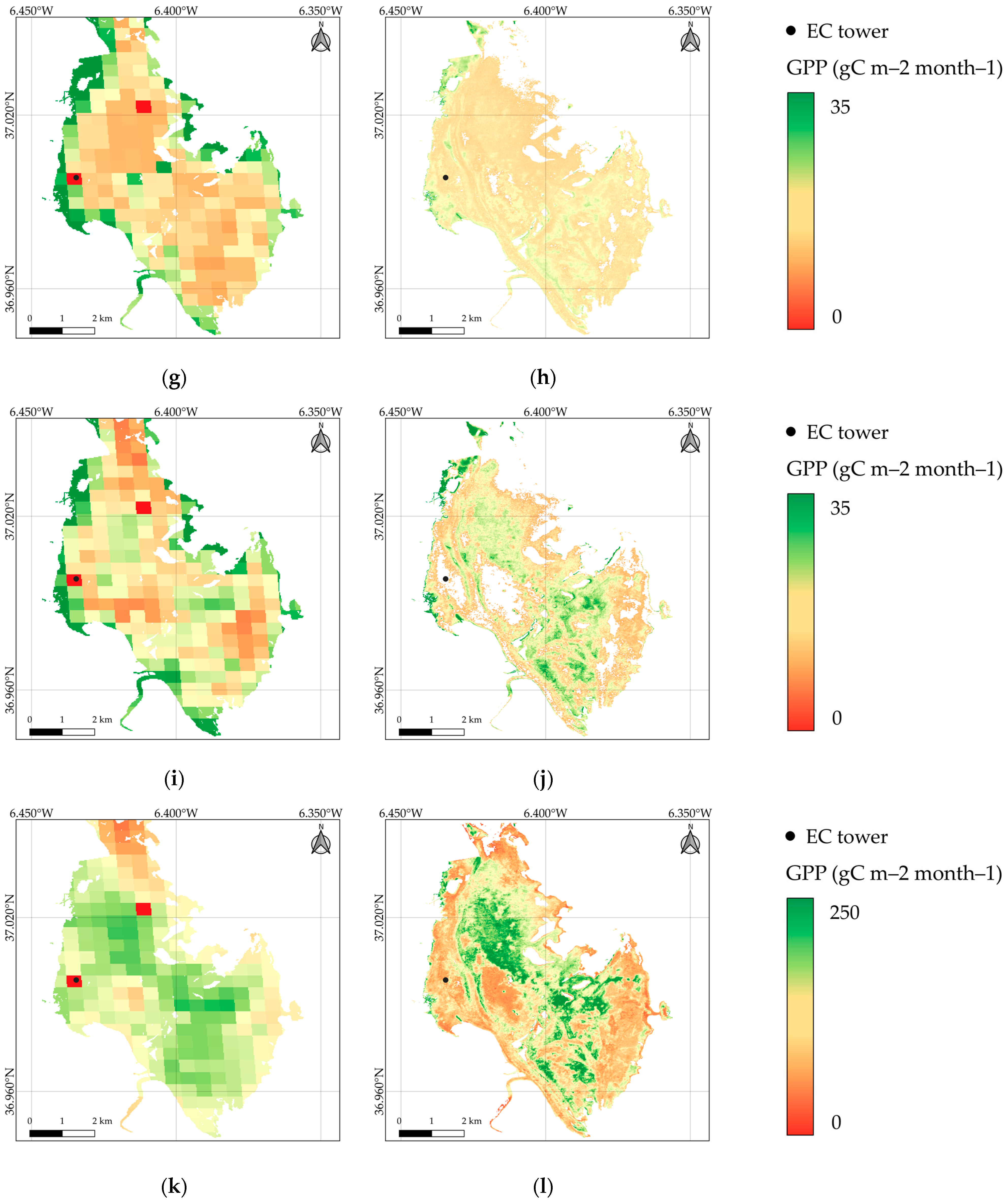
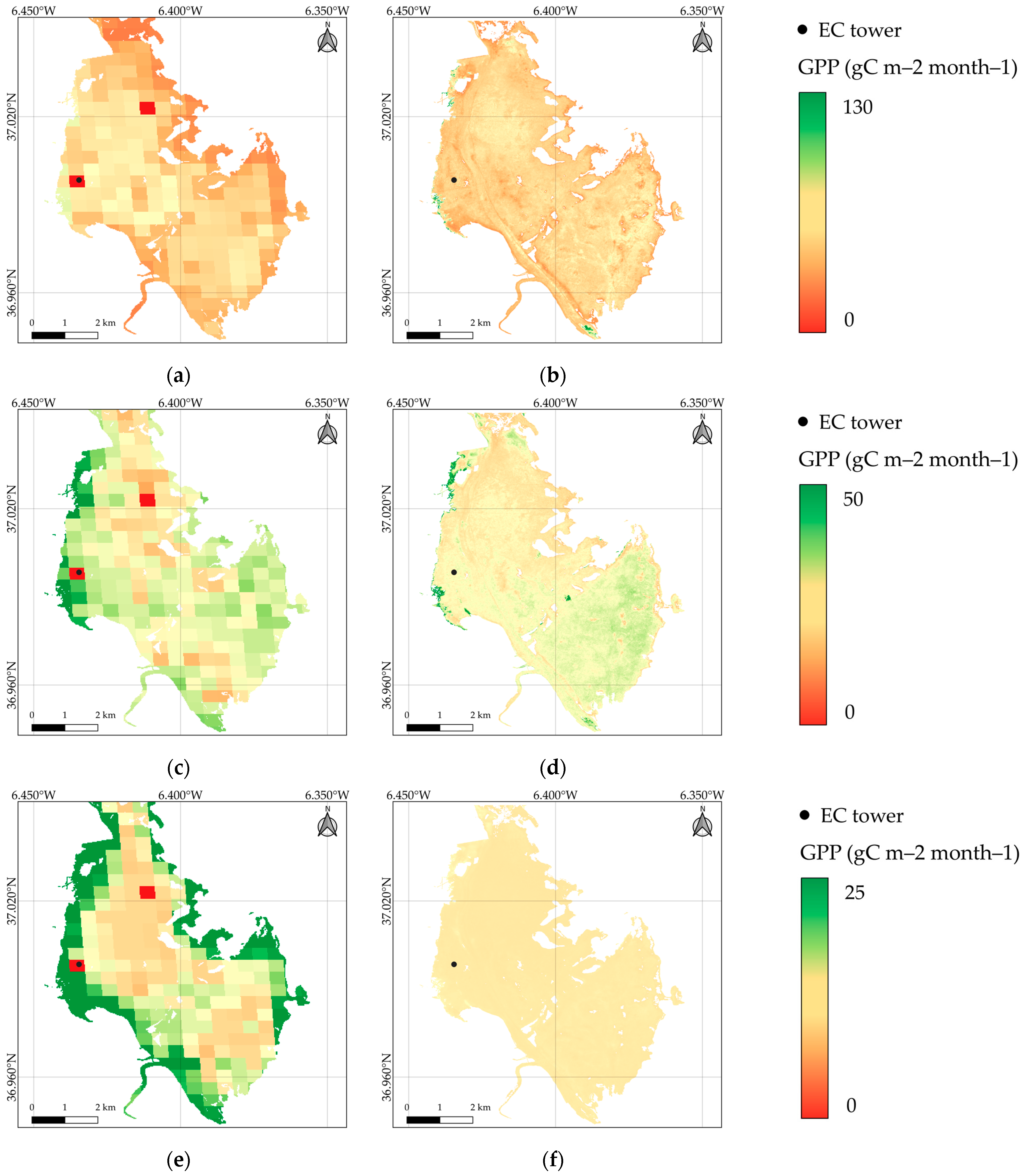
Figure A1. Comparison of Sentinel-2 (S2) and MOD17 GPP maps obtained using a monthly composite image. The maps show the spatial and temporal pattern of GPP (gC m−2 month−1) and the difference captured by the two satellites given their different spatial resolution. (a) MOD17 October 2020, (b) S2 October 2020, (c) MOD17 November 2020, (d) S2 November 2020, (e) MOD17 December 2020, (f) S2 December 2020, (g) MOD17 January 2021, (h) S2 January 2021, (i) MOD17 February 2021, (j) S2 February 2021, (k) MOD17 March 2021, (l) S2 March 2021, (m) MOD17 April 2021, (n) S2 April 2021, (o) MOD17 May 2021, (p) S2 May 2021.
Remotesensing 15 00562 g0a1aRemotesensing 15 00562 g0a1bRemotesensing 15 00562 g0a1c

References

  1. Orradóttir, B.; Aegisdóttir, H.H. Healthy Ecosystems, Healthy Earth, Healthy People. United Nations University. 2015. Available online: https://unu.edu/publications/articles/healthy-ecosystems-earth-people.html (accessed on 12 December 2022).
  2. United Nations Transforming Our World: The 2030 Agenda for Sustainable Development. United Nations Department of Economic and Social Affairs. 2015. Available online: https://sdgs.un.org/2030agenda (accessed on 12 December 2022).
  3. Agreement, P. Report of the Conference of the Parties to the United Nations Framework Convention on Climate Change (21st Session, 2015: Paris). Paris Agreement. Retrived December; HeinOnline. 2015, p. 2017. Available online: https://heinonline.org/HOL/LandingPage?handle=hein.journals/intlm55&div=46&id=&page= (accessed on 12 December 2022).
  4. Pereira, H.M.; Ferrier, S.; Walters, M.; Geller, G.N.; Jongman, R.; Scholes, R.J.; Bruford, M.W.; Brummitt, N.; Butchart, S.; Cardoso, A. Essential biodiversity variables. Science 2013, 339, 277–278. [Google Scholar] [CrossRef] [PubMed] [Green Version]
  5. Convention on Biological Diversity. Decision X/2, The Strategic Plan for Biodiversity 2011–2020 and the Aichi Biodiversity Targets. In Proceedings of the Conference of the Parties to the Convention on Biological Diversity, Nagoya, Japan, 18–29 October 2010. [Google Scholar]
  6. Ishtiaque, A.; Masrur, A.; Rabby, Y.W.; Jerin, T.; Dewan, A. Remote sensing-based research for monitoring progress towards SDG 15 in Bangladesh: A review. Remote Sens. 2020, 12, 691. [Google Scholar] [CrossRef] [Green Version]
  7. Zeng, Y.; Hao, D.; Huete, A.; Dechant, B.; Berry, J.; Chen, J.M.; Joiner, J.; Frankenberg, C.; Bond-Lamberty, B.; Ryu, Y. Optical vegetation indices for monitoring terrestrial ecosystems globally. Nat. Rev. Earth Environ. 2022, 3, 477–493. [Google Scholar] [CrossRef]
  8. Zhang, Z.; Ju, W.; Zhou, Y. The effect of water stress on net primary productivity in northwest China. Environ. Sci. Pollut. Res. 2021, 28, 65885–65898. [Google Scholar] [CrossRef] [PubMed]
  9. Boelman, N.T.; Stieglitz, M.; Rueth, H.M.; Sommerkorn, M.; Griffin, K.L.; Shaver, G.R.; Gamon, J.A. Response of NDVI, biomass, and ecosystem gas exchange to long-term warming and fertilization in wet sedge tundra. Oecologia 2003, 135, 414–421. [Google Scholar] [CrossRef]
  10. El Serafy, G.Y.; Schaeffer, B.A.; Neely, M.-B.; Spinosa, A.; Odermatt, D.; Weathers, K.C.; Baracchini, T.; Bouffard, D.; Carvalho, L.; Conmy, R.N. Integrating inland and coastal water quality data for actionable knowledge. Remote Sens. 2021, 13, 2899. [Google Scholar] [CrossRef]
  11. Soubry, I.; Doan, T.; Chu, T.; Guo, X. A systematic review on the integration of remote sensing and gis to forest and grassland ecosystem health attributes, indicators, and measures. Remote Sens. 2021, 13, 3262. [Google Scholar] [CrossRef]
  12. Paganini, M.; Leidner, A.K.; Geller, G.; Turner, W.; Wegmann, M. The role of space agencies in remotely sensed essential biodiversity variables. Remote Sens. Ecol. Conserv. 2016, 2, 132–140. [Google Scholar] [CrossRef]
  13. Callicott, J.B.; Crowder, L.B.; Mumford, K. Current normative concepts in conservation. Conserv. Biol. 1999, 13, 22–35. [Google Scholar] [CrossRef]
  14. Magurran, A.E. Biological diversity. Curr. Biol. 2005, 15, R116–R118. [Google Scholar] [CrossRef]
  15. Schröter, M.; Albert, C.; Marques, A.; Tobon, W.; Lavorel, S.; Maes, J.; Brown, C.; Klotz, S.; Bonn, A. National ecosystem assessments in Europe: A review. BioScience 2016, 66, 813–828. [Google Scholar] [CrossRef] [Green Version]
  16. Escribano, P.; Fernández, N. Ecosystem Functioning Observations for Assessing Conservation in the Doñana National Park, Spain. In Satellite Remote Sensing for Conservation Action. Case Studies from Aquatic and Terrestrial Ecosystems; Cambridge University Press: Cambridge, UK, 2018; Volume 164. [Google Scholar] [CrossRef]
  17. Li, Z.; Xu, D.; Guo, X. Remote sensing of ecosystem health: Opportunities, challenges, and future perspectives. Sensors 2014, 14, 21117–21139. [Google Scholar] [CrossRef] [PubMed] [Green Version]
  18. Norkko, A.; Villnäs, A.; Norkko, J.; Valanko, S.; Pilditch, C. Size matters: Implications of the loss of large individuals for ecosystem function. Sci. Rep. 2013, 3, 2646. [Google Scholar] [CrossRef] [PubMed] [Green Version]
  19. Lovett, G.M.; Jones, C.G.; Turner, M.G.; Weathers, K.C. Ecosystem function in heterogeneous landscapes. In Ecosystem Function in Heterogeneous Landscapes; Springer: Berlin/Heidelberg, Germany, 2005; pp. 1–4. [Google Scholar] [CrossRef]
  20. Pettorelli, N.; Schulte to Bühne, H.; Tulloch, A.; Dubois, G.; Macinnis-Ng, C.; Queirós, A.M.; Keith, D.A.; Wegmann, M.; Schrodt, F.; Stellmes, M. Satellite remote sensing of ecosystem functions: Opportunities, challenges and way forward. Remote Sens. Ecol. Conserv. 2018, 4, 71–93. [Google Scholar] [CrossRef]
  21. Pettorelli, N.; Owen, H.J.F.; Duncan, C. How do we want Satellite Remote Sensing to support biodiversity conservation globally? Methods Ecol. Evol. 2016, 7, 656–665. [Google Scholar] [CrossRef]
  22. Wylie, B.K.; Johnson, D.A.; Laca, E.; Saliendra, N.Z.; Gilmanov, T.G.; Reed, B.C.; Tieszen, L.L.; Worstell, B.B. Calibration of remotely sensed, coarse resolution NDVI to CO2 fluxes in a sagebrush–steppe ecosystem. Remote Sens. Environ. 2003, 85, 243–255. [Google Scholar] [CrossRef]
  23. Olofsson, P.; Lagergren, F.; Lindroth, A.; Lindström, J.; Klemedtsson, L.; Kutsch, W.; Eklundh, L. Towards operational remote sensing of forest carbon balance across Northern Europe. Biogeosciences 2008, 5, 817–832. [Google Scholar] [CrossRef] [Green Version]
  24. Xu, C.; Li, Y.; Hu, J.; Yang, X.; Sheng, S.; Liu, M. Evaluating the difference between the normalized difference vegetation index and net primary productivity as the indicators of vegetation vigor assessment at landscape scale. Environ. Monit. Assess. 2012, 184, 1275–1286. [Google Scholar] [CrossRef]
  25. Cai, Z.; Junttila, S.; Holst, J.; Jin, H.; Ardö, J.; Ibrom, A.; Peichl, M.; Mölder, M.; Jönsson, P.; Rinne, J. Modelling daily gross primary productivity with sentinel-2 data in the nordic region–comparison with data from modis. Remote Sens. 2021, 13, 469. [Google Scholar] [CrossRef]
  26. Badgley, G.; Field, C.B.; Berry, J.A. Canopy near-infrared reflectance and terrestrial photosynthesis. Sci. Adv. 2017, 3, e1602244. [Google Scholar] [CrossRef] [Green Version]
  27. Badgley, G.; Anderegg, L.D.; Berry, J.A.; Field, C.B. Terrestrial gross primary production: Using NIRV to scale from site to globe. Glob. Chang. Biol. 2019, 25, 3731–3740. [Google Scholar] [CrossRef]
  28. Baldocchi, D.D.; Ryu, Y.; Dechant, B.; Eichelmann, E.; Hemes, K.; Ma, S.; Sanchez, C.R.; Shortt, R.; Szutu, D.; Valach, A. Outgoing near-infrared radiation from vegetation scales with canopy photosynthesis across a spectrum of function, structure, physiological capacity, and weather. J. Geophys. Res. Biogeosci. 2020, 125, e2019JG005534. [Google Scholar] [CrossRef]
  29. Wang, S.; Zhang, Y.; Ju, W.; Qiu, B.; Zhang, Z. Tracking the seasonal and inter-annual variations of global gross primary production during last four decades using satellite near-infrared reflectance data. Sci. Total Environ. 2021, 755, 142569. [Google Scholar] [CrossRef] [PubMed]
  30. Wu, G.; Guan, K.; Jiang, C.; Peng, B.; Kimm, H.; Chen, M.; Yang, X.; Wang, S.; Suyker, A.E.; Bernacchi, C.J. Radiance-based NIRv as a proxy for GPP of corn and soybean. Environ. Res. Lett. 2020, 15, 034009. [Google Scholar] [CrossRef]
  31. Yin, G.; Verger, A.; Descals, A.; Filella, I.; Peñuelas, J. A broadband green-red vegetation index for monitoring gross primary production phenology. J. Remote Sens. 2022, 2022, 1–10. [Google Scholar] [CrossRef]
  32. Cerasoli, S.; Campagnolo, M.; Faria, J.; Nogueira, C.; Caldeira, M.d.C. On estimating the gross primary productivity of Mediterranean grasslands under different fertilization regimes using vegetation indices and hyperspectral reflectance. Biogeosciences 2018, 15, 5455–5471. [Google Scholar] [CrossRef] [Green Version]
  33. Lin, S.; Li, J.; Liu, Q.; Li, L.; Zhao, J.; Yu, W. Evaluating the effectiveness of using vegetation indices based on red-edge reflectance from Sentinel-2 to estimate gross primary productivity. Remote Sens. 2019, 11, 1303. [Google Scholar] [CrossRef] [Green Version]
  34. Noumonvi, K.D.; Ferlan, M.; Eler, K.; Alberti, G.; Peressotti, A.; Cerasoli, S. Estimation of carbon fluxes from eddy covariance data and satellite-derived vegetation indices in a karst grassland (Podgorski Kras, Slovenia). Remote Sens. 2019, 11, 649. [Google Scholar] [CrossRef]
  35. Robinson, N.P.; Allred, B.W.; Smith, W.K.; Jones, M.O.; Moreno, A.; Erickson, T.A.; Naugle, D.E.; Running, S.W. Terrestrial primary production for the conterminous United States derived from Landsat 30 m and MODIS 250 m. Remote Sens. Ecol. Conserv. 2018, 4, 264–280. [Google Scholar] [CrossRef]
  36. Running, S.W.; Nemani, R.R.; Heinsch, F.A.; Zhao, M.; Reeves, M.C.; Hashimoto, H. A Continuous Satellite-Derived Measure of Global Terrestrial Primary Production. Bioscience 2004, 54, 547–560. [Google Scholar] [CrossRef]
  37. Zhao, M.; Heinsch, F.A.; Nemani, R.R.; Running, S.W. Improvements of the MODIS terrestrial gross and net primary production global data set. Remote Sens. Environ. 2005, 95, 164–176. [Google Scholar] [CrossRef]
  38. Zhu, H.; Lin, A.; Wang, L.; Xia, Y.; Zou, L. Evaluation of MODIS gross primary production across multiple biomes in China using eddy covariance flux data. Remote Sens. 2016, 8, 395. [Google Scholar] [CrossRef] [Green Version]
  39. Heinsch, F.A.; Maosheng, Z.; Running, S.W.; Kimball, J.S.; Nemani, R.R.; Davis, K.J.; Bolstad, P.V.; Cook, B.D.; Desai, A.R.; Ricciuto, D.M.; et al. Evaluation of remote sensing based terrestrial productivity from MODIS using regional tower eddy flux network observations. IEEE Trans. Geosci. Remote Sens. 2006, 44, 1908–1925. [Google Scholar] [CrossRef] [Green Version]
  40. Turner, D.P.; Ritts, W.D.; Cohen, W.B.; Gower, S.T.; Zhao, M.; Running, S.W.; Wofsy, S.C.; Urbanski, S.; Dunn, A.L.; Munger, J. Scaling gross primary production (GPP) over boreal and deciduous forest landscapes in support of MODIS GPP product validation. Remote Sens. Environ. 2003, 88, 256–270. [Google Scholar] [CrossRef] [Green Version]
  41. Balzarolo, M.; Peñuelas, J.; Veroustraete, F. Influence of landscape heterogeneity and spatial resolution in multi-temporal in situ and MODIS NDVI data proxies for seasonal GPP dynamics. Remote Sens. 2019, 11, 1656. [Google Scholar] [CrossRef] [Green Version]
  42. Wang, S.; Garcia, M.; Bauer-Gottwein, P.; Jakobsen, J.; Zarco-Tejada, P.J.; Bandini, F.; Paz, V.S.; Ibrom, A. High spatial resolution monitoring land surface energy, water and CO2 fluxes from an Unmanned Aerial System. Remote Sens. Environ. 2019, 229, 14–31. [Google Scholar] [CrossRef]
  43. Neumann, M.; Moreno, A.; Thurnher, C.; Mues, V.; Härkönen, S.; Mura, M.; Bouriaud, O.; Lang, M.; Cardellini, G.; Thivolle-Cazat, A. Creating a regional MODIS satellite-driven net primary production dataset for European forests. Remote Sens. 2016, 8, 554. [Google Scholar] [CrossRef] [Green Version]
  44. Running, S.W.; Thornton, P.E.; Nemani, R.; Glassy, J.M. Global terrestrial gross and net primary productivity from the earth observing system. In Methods in Ecosystem Science; Springer: Berlin/Heidelberg, Germany, 2000; pp. 44–57. [Google Scholar] [CrossRef]
  45. Schubert, P.; Lagergren, F.; Aurela, M.; Christensen, T.; Grelle, A.; Heliasz, M.; Klemedtsson, L.; Lindroth, A.; Pilegaard, K.; Vesala, T. Modeling GPP in the Nordic forest landscape with MODIS time series data—Comparison with the MODIS GPP product. Remote Sens. Environ. 2012, 126, 136–147. [Google Scholar] [CrossRef]
  46. Sims, D.A.; Rahman, A.F.; Cordova, V.D.; El-Masri, B.Z.; Baldocchi, D.D.; Flanagan, L.B.; Goldstein, A.H.; Hollinger, D.Y.; Misson, L.; Monson, R.K. On the use of MODIS EVI to assess gross primary productivity of North American ecosystems. J. Geophys. Res. Biogeosci. 2006, 111. [Google Scholar] [CrossRef] [Green Version]
  47. Secretariat, R.C. The Ramsar Convention Manual: A Guide to the Convention on Wetlands (Ramsar, Iran, 1971); Ramsar Convention Secretariat: Gland, Switzerland, 2013; Available online: https://www.ramsar.org/sites/default/files/documents/library/manual6-2013-e.pdf (accessed on 12 December 2022).
  48. Green, A.J.; Bustamante, J.; Janss, G.F.E.; Fernández-Zamudio, R.; Díaz-Paniagua, C. Doñana Wetlands (Spain). In The Wetland Book: II: Distribution, Description and Conservation; Finlayson, C.M., Milton, G.R., Prentice, R.C., Davidson, N.C., Eds.; Springer Netherlands: Dordrecht, The Netherlands, 2016; pp. 1–14. [Google Scholar] [CrossRef] [Green Version]
  49. García Novo, F.; Marín Cabrera, C. Doñana: Water and Biosphere, Doñana 2005 Project. Guadalquivir Hydrol. Basin Auth. Span. Minist. Environ. Madr. 2006. Available online: https://www.researchgate.net/profile/Francisco-Barrera-6/publication/260990490_Donana_Water_and_Biosphere/links/0a85e532f31a8515d9000000/Donana-Water-and-Biosphere.pdf (accessed on 12 December 2022).
  50. Green, A.J.; Elmberg, J. Ecosystem services provided by waterbirds. Biol. Rev. 2014, 89, 105–122. [Google Scholar] [CrossRef] [Green Version]
  51. Hernández, L.M.; Gómara, B.; Fernández, M.; Jiménez, B.; González, M.; Baos, R.; Hiraldo, F.; Ferrer, M.; Benito, V.; Suner, M. Accumulation of heavy metals and As in wetland birds in the area around Donana National Park affected by the Aznalcollar toxic spill. Sci. Total Environ. 1999, 242, 293–308. [Google Scholar] [CrossRef]
  52. Pain, D.; Sánchez, A.; Meharg, A. The Donana ecological disaster: Contamination of a world heritage estuarine marsh ecosystem with acidified pyrite mine waste. Sci. Total Environ. 1998, 222, 45–54. [Google Scholar] [CrossRef]
  53. Adame, J.A.; Lope, L.; Hidalgo, P.J.; Sorribas, M.; Gutiérrez-Álvarez, I.; del Águila, A.; Saiz-Lopez, A.; Yela, M. Study of the exceptional meteorological conditions, trace gases and particulate matter measured during the 2017 forest fire in Doñana Natural Park, Spain. Sci. Total Environ. 2018, 645, 710–720. [Google Scholar] [CrossRef] [PubMed]
  54. Informe, W. Contaminación del agua en Doñana. Evaluación De Los Vertidos Sin Depurar De Los Munic. De Almonte Rociana Del Condado Y Bollullos Par Del Contado (Comarc. De Doñana Huelva); WWF: New York, NY, USA, 2012; Available online: https://www.wwf.es/?28640/Impactantes-imgenes-de-WWF-demuestran--cmo-las-cloacas-vierten-directamente-a-Doana (accessed on 12 December 2022).
  55. Taggart, M.A.; Figuerola, J.; Green, A.J.; Mateo, R.; Deacon, C.; Osborn, D.; Meharg, A.A. After the Aznalcóllar mine spill: Arsenic, zinc, selenium, lead and copper levels in the livers and bones of five waterfowl species. Environ. Res. 2006, 100, 349–361. [Google Scholar] [CrossRef]
  56. Guardiola-Albert, C.; Jackson, C.R. Potential impacts of climate change on groundwater supplies to the Doñana wetland, Spain. Wetlands 2011, 31, 907–920. [Google Scholar] [CrossRef] [Green Version]
  57. Manzano, M.; Custodio, E.; Lozano, E.; Higueras, H. Relationships between wetlands and the Doñana coastal aquifer (SW Spain). Groundw. Ecosyst. 2013, 169, 169–182. [Google Scholar] [CrossRef]
  58. Lumbierres, M.; Méndez, P.F.; Bustamante, J.; Soriguer, R.; Santamaría, L. Modeling biomass production in seasonal wetlands using MODIS NDVI land surface phenology. Remote Sens. 2017, 9, 392. [Google Scholar] [CrossRef] [Green Version]
  59. Kordelas, G.A.; Manakos, I.; Aragonés, D.; Díaz-Delgado, R.; Bustamante, J. Fast and Automatic Data-Driven Thresholding for Inundation Mapping with Sentinel-2 Data. Remote Sens. 2018, 10, 910. [Google Scholar] [CrossRef] [Green Version]
  60. Papale, D.; Reichstein, M.; Aubinet, M.; Canfora, E.; Bernhofer, C.; Kutsch, W.; Longdoz, B.; Rambal, S.; Valentini, R.; Vesala, T. Towards a standardized processing of Net Ecosystem Exchange measured with eddy covariance technique: Algorithms and uncertainty estimation. Biogeosciences 2006, 3, 571–583. [Google Scholar] [CrossRef] [Green Version]
  61. Cuntz, M. hesseflux: A Python library to process and post-process Eddy covariance data. 2020. [Google Scholar]
  62. Forbrich, I.; Giblin, A.E. Marsh-atmosphere CO2 exchange in a New England salt marsh. J. Geophys. Res. Biogeosci. 2015, 120, 1825–1838. [Google Scholar] [CrossRef] [Green Version]
  63. Kljun, N.; Calanca, P.; Rotach, M.; Schmid, H. The simple two-dimensional parameterisation for Flux Footprint Predictions FFP. Geosci. Model Dev. Discuss. 2015, 8, 3695–3713. [Google Scholar] [CrossRef] [Green Version]
  64. Sathe, A.; Mann, J.; Gottschall, J.; Courtney, M. Estimating the Systematic Errors in Turbulence Sensed by Wind Lidars; Risø National Laboratory: Risø, Denmark, 2010.
  65. Allen, R.G.; Pereira, L.S.; Howell, T.A.; Jensen, M.E. Evapotranspiration information reporting: I. Factors governing measurement accuracy. Agric. Water Manag. 2011, 98, 899–920. [Google Scholar] [CrossRef] [Green Version]
  66. Akima, H. A new method of interpolation and smooth curve fitting based on local procedures. J. ACM (JACM) 1970, 17, 589–602. [Google Scholar] [CrossRef]
  67. Churkina, G.; Running, S.W.; Schloss, A.L.; Participants Potsdam, N.P.P.M.I. Comparing global models of terrestrial net primary productivity (NPP): The importance of water availability. Glob. Chang. Biol. 1999, 5, 46–55. [Google Scholar] [CrossRef]
  68. Díaz-Delgado, R.; Carro, F.; Quirós, F.; Osuna, A.; Baena-Capilla, M. Contribution from Long-Term Ecological Monitoring to research and management of Doñana LTSER Platform. Asoc. Española De Ecol. Terr. 2016, 25, 9–18. [Google Scholar] [CrossRef] [Green Version]
  69. Huertas, I.E.; Flecha, S.; Figuerola, J.; Costas, E.; Morris, E.P. Effect of hydroperiod on CO2 fluxes at the air-water interface in the Mediterranean coastal wetlands of Doñana. J. Geophys. Res. Biogeosci. 2017, 122, 1615–1631. [Google Scholar] [CrossRef]
  70. Arthur, D.; Vassilvitskii, S. k-means++: The Advantages of Careful Seeding; Stanford InfoLab: Stanford, CA, USA, 2006; Available online: http://ilpubs.stanford.edu:8090/778/ (accessed on 12 December 2022).
  71. dela Torre, D.M.G.; Gao, J.; Macinnis-Ng, C.; Shi, Y. Phenology-based delineation of irrigated and rain-fed paddy fields with Sentinel-2 imagery in Google Earth Engine. Geo-Spat. Inf. Sci. 2021, 24, 695–710. [Google Scholar] [CrossRef]
  72. Sharma, R.; Ghosh, A.; Joshi, P.K. Decision tree approach for classification of remotely sensed satellite data using open source support. J. Earth Syst. Sci. 2013, 122, 1237–1247. [Google Scholar] [CrossRef] [Green Version]
  73. Yang, L.; Driscol, J.; Sarigai, S.; Wu, Q.; Chen, H.; Lippitt, C.D. Google Earth Engine and Artificial Intelligence (AI): A Comprehensive Review. Remote Sens. 2022, 14, 3253. Available online: https://www.mdpi.com/2072-4292/14/14/3253 (accessed on 12 December 2022). [CrossRef]
  74. Domingo, M.S.; Martín-Perea, D.M.; Badgley, C.; Cantero, E.; López-Guerrero, P.; Oliver, A.; Negro, J.J. Taphonomic information from the modern vertebrate death assemblage of Doñana National Park, Spain. PLoS ONE 2020, 15, e0242082. [Google Scholar] [CrossRef] [PubMed]
  75. Serrano, L. Balancing water uses at the Donana national park, Spain. In The Wetland Book: I: Structure and Function, Management and Methods; Finlayson, C.M., Everard, M., Irvine, K., McInnes, R.J., Middleton, B.A., van Dam, A.A., Davidson, N.C., Eds.; Springer: Dordrecht, The Netherlands, 2016; pp. 1–8. [Google Scholar] [CrossRef]
  76. Blackburn, G.A.; Pitman, J. Biophysical controls on the directional spectral reflectance properties of bracken (Pteridium aquilinum) canopies: Results of a field experiment. Int. J. Remote Sens. 1999, 20, 2265–2282. [Google Scholar] [CrossRef]
  77. Mutanga, O.; Skidmore, A.K.; Van Wieren, S. Discriminating tropical grass (Cenchrus ciliaris) canopies grown under different nitrogen treatments using spectroradiometry. ISPRS J. Photogramm. Remote Sens. 2003, 57, 263–272. [Google Scholar] [CrossRef]
  78. Thenkabail, P.S.; Smith, R.B.; De Pauw, E. Hyperspectral vegetation indices and their relationships with agricultural crop characteristics. Remote Sens. Environ. 2000, 71, 158–182. [Google Scholar] [CrossRef]
  79. Gianelle, D.; Vescovo, L. Determination of green herbage ratio in grasslands using spectral reflectance. Methods and ground measurements. Int. J. Remote Sens. 2007, 28, 931–942. [Google Scholar] [CrossRef]
  80. Mutanga, O.; Skidmore, A.K. Narrow band vegetation indices overcome the saturation problem in biomass estimation. Int. J. Remote Sens. 2004, 25, 3999–4014. [Google Scholar] [CrossRef]
  81. Huete, A.; Didan, K.; Miura, T.; Rodriguez, E.P.; Gao, X.; Ferreira, L.G. Overview of the radiometric and biophysical performance of the MODIS vegetation indices. Remote Sens. Environ. 2002, 83, 195–213. [Google Scholar] [CrossRef]
  82. Reed, B.C.; Schwartz, M.D.; Xiao, X. Remote Sensing Phenology. In Phenology of Ecosystem Processes: Applications in Global Change Research; Noormets, A., Ed.; Springer New York: New York, NY, USA, 2009; pp. 231–246. [Google Scholar] [CrossRef]
  83. Bajgain, R.; Xiao, X.; Wagle, P.; Basara, J.; Zhou, Y. Sensitivity analysis of vegetation indices to drought over two tallgrass prairie sites. ISPRS J. Photogramm. Remote Sens. 2015, 108, 151–160. [Google Scholar] [CrossRef]
  84. Máñez, M.; García, L.; Ibáñez, F.; Garrido, H.; Espinar, J.M.; Arroyo, J.L.; Valle, J.L.D.; Chico, A.; Martínez, A.; Rodríguez, R. Endangered waterbirds at Doñana natural space. Conserv. Monit. Freshw. Habitats 2010, 357–373. [Google Scholar] [CrossRef] [Green Version]
  85. Flood, N. Seasonal composite Landsat TM/ETM+ images using the medoid (a multi-dimensional median). Remote Sens. 2013, 5, 6481–6500. [Google Scholar] [CrossRef] [Green Version]
  86. Duveiller, G.; Cescatti, A. Spatially downscaling sun-induced chlorophyll fluorescence leads to an improved temporal correlation with gross primary productivity. Remote Sens. Environ. 2016, 182, 72–89. [Google Scholar] [CrossRef]
  87. Glenn, E.P.; Huete, A.R.; Nagler, P.L.; Nelson, S.G. Relationship Between Remotely-sensed Vegetation Indices, Canopy Attributes and Plant Physiological Processes: What Vegetation Indices Can and Cannot Tell Us About the Landscape. Sensors 2008, 8, 2136–2160. [Google Scholar] [CrossRef] [PubMed] [Green Version]
  88. Wang, Y.; Woodcock, C.E.; Buermann, W.; Stenberg, P.; Voipio, P.; Smolander, H.; Häme, T.; Tian, Y.; Hu, J.; Knyazikhin, Y.; et al. Evaluation of the MODIS LAI algorithm at a coniferous forest site in Finland. Remote Sens. Environ. 2004, 91, 114–127. [Google Scholar] [CrossRef]
  89. Gelybó, G.; Barcza, Z.; Kern, A.; Kljun, N. Effect of spatial heterogeneity on the validation of remote sensing based GPP estimations. Agric. For. Meteorol. 2013, 174–175, 43–53. [Google Scholar] [CrossRef]
  90. Duda, T.; Canty, M. Unsupervised classification of satellite imagery: Choosing a good algorithm. Int. J. Remote Sens. 2002, 23, 2193–2212. [Google Scholar] [CrossRef]
  91. Hasmadi, M.; Pakhriazad, H.; Shahrin, M. Evaluating supervised and unsupervised techniques for land cover mapping using remote sensing data. Geogr. Malays. J. Soc. Space 2009, 5, 1–10. [Google Scholar]
  92. Meroni, M.; Fasbender, D.; Lopez-Lozano, R.; Migliavacca, M. Assimilation of Earth observation data over cropland and grassland sites into a simple GPP model. Remote Sens. 2019, 11, 749. [Google Scholar] [CrossRef] [Green Version]
  93. Reichstein, M.; Falge, E.; Baldocchi, D.; Papale, D.; Aubinet, M.; Berbigier, P.; Bernhofer, C.; Buchmann, N.; Gilmanov, T.; Granier, A. On the separation of net ecosystem exchange into assimilation and ecosystem respiration: Review and improved algorithm. Glob. Chang. Biol. 2005, 11, 1424–1439. [Google Scholar] [CrossRef]
  94. Lasslop, G.; Reichstein, M.; Papale, D.; Richardson, A.D.; Arneth, A.; Barr, A.; Stoy, P.; Wohlfahrt, G. Separation of net ecosystem exchange into assimilation and respiration using a light response curve approach: Critical issues and global evaluation. Glob. Chang. Biol. 2010, 16, 187–208. [Google Scholar] [CrossRef] [Green Version]
  95. Falge, E.; Baldocchi, D.; Olson, R.; Anthoni, P.; Aubinet, M.; Bernhofer, C.; Burba, G.; Ceulemans, R.; Clement, R.; Dolman, H. Gap filling strategies for defensible annual sums of net ecosystem exchange. Agric. For. Meteorol. 2001, 107, 43–69. [Google Scholar] [CrossRef] [Green Version]
  96. Rocha, A.V.; Goulden, M.L. Why is marsh productivity so high? New insights from eddy covariance and biomass measurements in a Typha marsh. Agric. For. Meteorol. 2009, 149, 159–168. [Google Scholar] [CrossRef] [Green Version]
  97. Lasslop, G.; Reichstein, M.; Kattge, J.; Papale, D. Influences of observation errors in eddy flux data on inverse model parameter estimation. Biogeosciences 2008, 5, 1311–1324. [Google Scholar] [CrossRef] [Green Version]
  98. Zhu, W.; Pan, Y.; He, H.; Wang, L.; Mou, M.; Liu, J. A changing-weight filter method for reconstructing a high-quality NDVI time series to preserve the integrity of vegetation phenology. IEEE Trans. Geosci. Remote Sens. 2011, 50, 21085–21094. [Google Scholar] [CrossRef]
  99. Chen, J.; Jönsson, P.; Tamura, M.; Gu, Z.; Matsushita, B.; Eklundh, L. A simple method for reconstructing a high-quality NDVI time-series data set based on the Savitzky–Golay filter. Remote Sens. Environ. 2004, 91, 332–344. [Google Scholar] [CrossRef]
  100. Jonsson, P.; Eklundh, L. Seasonality extraction by function fitting to time-series of satellite sensor data. IEEE Trans. Geosci. Remote Sens. 2002, 40, 1824–1832. [Google Scholar] [CrossRef]
  101. Beck, P.S.; Atzberger, C.; Høgda, K.A.; Johansen, B.; Skidmore, A.K. Improved monitoring of vegetation dynamics at very high latitudes: A new method using MODIS NDVI. Remote Sens. Environ. 2006, 100, 321–334. [Google Scholar] [CrossRef]
  102. Viovy, N.; Arino, O.; Belward, A. The Best Index Slope Extraction (BISE): A method for reducing noise in NDVI time-series. Int. J. Remote Sens. 1992, 13, 1585–1590. [Google Scholar] [CrossRef]
  103. Rouse, J.W.; Haas, R.H.; Schell, J.A.; Deering, D.W. Monitoring Vegetation Systems in the Great Plains with Erts. Nasa Spec. Publ. 1974, 351, 309. [Google Scholar]
  104. Jiang, Z.; Huete, A.R.; Didan, K.; Miura, T. Development of a two-band enhanced vegetation index without a blue band. Remote Sens. Environ. 2008, 112, 3833–3845. [Google Scholar] [CrossRef]
  105. Xu, H. Modification of normalised difference water index (NDWI) to enhance open water features in remotely sensed imagery. Int. J. Remote Sens. 2006, 27, 3025–3033. [Google Scholar] [CrossRef]
  106. Adan, M.S. Integrating Sentinel-2 Derived Vegetation Indices and Terrestrial Laser Scanner to Estimate Above-Ground Biomass/Carbon in Ayer Hitam Tropical Forest Malaysia. Master’s Thesis, University of Twente, Enschede, The Netherlands, 2017. Available online: http://essay.utwente.nl/83579/1/adan.pdf (accessed on 12 December 2022).
  107. Gao, B.-c. NDWI—A normalized difference water index for remote sensing of vegetation liquid water from space. Remote Sens. Environ. 1996, 58, 257–266. [Google Scholar] [CrossRef]
  108. Hardisky, M.A.; Klemas, V.; Smart, R. The influence of soil salinity, growth form, and leaf moisture on-the spectral radiance of. Photogramm. Eng. Remote Sens 1983, 49, 77–83. Available online: https://www.asprs.org/wp-content/uploads/pers/1983journal/jan/1983_jan_77-83.pdf (accessed on 12 December 2022).
Figure 1. Protected area limits of Doñana Natural Park and Doñana National Park located in the southwest of Spain, and the distribution of its major habitats.
Remotesensing 15 00562 g001
Figure 2. Tiles of Sentine-2 products over the study area of Doñana National Park. [Image retrieved from the Copernicus Open Access Hub].
Remotesensing 15 00562 g002
Figure 3. Schematization of methodology with details of data requirements (blue), data pre-processing (yellow), modeling processing (gray), and post-process and workflow outputs (green).
Remotesensing 15 00562 g003
Figure 4. Climatological footprint of 2020 (left image) and 2021 (right image).
Remotesensing 15 00562 g004
Figure 5. Schematization of the processing chain applied on the Sentinel-2 images to obtain the VIs time series. At first, S2 L2A images (with orthorectification and atmospheric correction) are collected and filtered by cloud coverage (<30%). Then, pixels are filtered using (i) the supplementary band QA60 to mask the clouds; (ii) the SCL band to select pixels classified as vegetation, soil and water and (iii) a water mask to remove flooded pixels without standing vegetation (MNDVI < 0.05). Finally, the VI is calculated for each pixel within the climatological footprint, multiplied by their contribution weight and summed to obtain the final VI, a single value of VI per image per day. The Akima fitting algorithm is then applied to fill in the gaps and obtain a continuous time series.
Remotesensing 15 00562 g005
Figure 6. Scatter plot and corresponding regression line and 95% confidence interval for the relationship between the GPP calculated as the product between the Red-edge index (CLr) and the rainfall data calculated with a rolling average of 90 days and delay of five months (RAIN_90_150) and the ground measurements of GPP.
Remotesensing 15 00562 g006
Figure 7. Scatter plot with fitted regression line showing the correlation between the predicted GPP values (x-axis) obtained by our model and the observed GPP values (y-axis).
Remotesensing 15 00562 g007
Figure 8. Scatter plot with fitted regression line showing the correlation between the predicted GPP MOD17 predictions (x-axis) and the observed GPP values (y-axis).
Remotesensing 15 00562 g008
Figure 9. Time series of our model GPP predictions, MOD17 GPP prediction and in situ measurements of GPP.
Remotesensing 15 00562 g009
Figure 10. Vegetation classification maps showing the seven classed identified by k-means algorithm implemented in Google Earth Engine API and ee. python package using a Sentinel-2 L2A mean composite image from the 1 October 2020 to the 31 May 2021. Class 1 and 2 correspond to the dense vegetated area, mainly dominated by the Cyperus rotundus, and the Cyperus rotundus and Sarcocornietea fruticosae plants, respectively. Class 3 is a vegetated area mainly dominated by the Cyperus rotundus. Class 4 and 5 are sand depression areas mainly characterized by salt marshes and shrubs and salt marshes, respectively. Class 6 and 7 correspond to ponds, temporarily and permanently flooded areas, respectively.
Remotesensing 15 00562 g010
Figure 11. Vegetation classification over the Doñana park for 2009 (shapefiles provided by ICTS-RBD). The Bolboschoenus maritimus vegetation identified in 2009 is displayed in orange. The “BM Lumbierres et al., 2017” red limited area represents the Bolboschoenus maritimus dominated area identified by Lumbierres et al. [58] and used in their research on biomass production. The red limited area has been adopted in our study for the estimation of GPP in the marsh area surrounding the EC tower.
Remotesensing 15 00562 g011
Figure 12. Monthly GPP maps obtained using a single composite image per month. The maps show the spatial and temporal pattern of GPP (gC m−2 month−1). (a) October 2020, (b) November 2020, (c) December 2020, (d) January 2021, (e) February 2021, (f) March 2021, (g) April 2021, (h) May 2021.
Remotesensing 15 00562 g012
Figure 13. Time series of the CLr index for different pixels in the upscaling area (pointers) and for the eddy covariance footprint (black dot).
Remotesensing 15 00562 g013
Figure 14. 15-days GPP maps. The maps show the spatial and temporal pattern of GPP (gC m−2 15-days−1). (a) 1–15 October 2020, (b) 16–31 October 2020, (c) 1–15 November 2020, (d) 16–30 November 2020, (e) 1–15 December 2020, (f) 16–31 December 2020, (g) 1–15 January 2021, (h) 16–31 January 2021.
Remotesensing 15 00562 g014
Figure 15. 15-days GPP maps. The maps show the spatial and temporal pattern of GPP (gC m−2 15-days−1). (a) 1–15 February 2021, (b) 16–28 February 2021, (c) 1–15 March 2021, (d) 16–31 March 2021, (e) 1–15 April 2021, (f) 16–30 April 2021, (g) 1–15 May 2021, (h) 16–31 May 2021.
Remotesensing 15 00562 g015
Figure 16. GPP map for the period October 2020 to May 2021 over the study area.
Remotesensing 15 00562 g016
Table 1. Data collected from the ICTS-RBD monitoring system.
DataTime RangeDescriptionVariablesUnits
Eddy covariance datafrom 1 October 2020
to 8 June 2021
Pre-processed eddy covariance measurements. Corrected 30-min estimations of gas analyzer and anemometer data.CO2 fluxµmol m−2 s−1
Quality flag CO2 flux-
Air temperatureK
Relative humidity%
Vapour pressure deficitPa
Friction velocitym s−1
Monin–Obukhov lengthM
Wind speedm s−1
Maximum wind speedm s−1
Wind direction° (degrees)
Variance of the wind component
along the v anemometer axis
m s−1
Meteorological datafrom 1 September 1976
to 31 October 2021
Daily estimations of meteorological data from analogic instruments.Rainfallmm
Maximum temperature°C
Minimum temperature°C
Mean temperature°C
Thermal oscillation°C
Table 2. Metadata of the ICTS-RBD monitoring system.
StationMetadata
Duque Fuente flux towerLocation36.9985 N, −6.4345 E
Canopy height0.7 m
Displacement height0.2 m
Roughness length-
Anemometer sensor height3.95 m
Gas analyser sensor height4.03 m
Tower fetch375 m
Anemometer sensor typeGill HS-50
Gas analyser sensortypeLI-7200 Enclosed CO2/H2O analyser
Palacio Doñana meteorological stationLocation36.9905 N, −6.4426 E
Sensor typeManual analogic instruments
Table 3. Available Sentinel-2 images from October 2020 to June 2021 for different cloud coverage.
MonthCloud Coverage
<100%<50%<30%
T29SQAT29SQBT29SQAT29SQBT29SQAT29SQB
10-2020666553
11-2020665445
12-2020664544
01-2021774433
02-2021551111
03-2021664646
04-2021662120
05-2021887755
06-2021665433
Total565638373130
Table 4. Environmental drivers of primary productivity used for the empirical model formulations.
VariableUnitsDescription
AT_MAX°CMaximum temperature
AT_MIN°CMinimum temperature
AT_MEAN°CDaily mean temperature
AT_OSC°CDaily thermal oscillation
AT_MEAN_f *°CDaily mean temperature
VPD_MEAN_fPaDaily mean of vapor pressure deficit
RAINmmDaily rainfall
RAIN_7mm30-days rainfall average
RAIN_15mm60-days rainfall average
RAIN_30mm30-days rainfall average
RAIN_60mm60-days rainfall average
RAIN_90mm90-days rainfall average
RAIN_7_N **mm7-day rainfall average with N-day lag
RAIN_15_Nmm15-day rainfall average with N-day lag
RAIN_30_Nmm30-day rainfall average with N-day lag
RAIN_60_Nmm60-day rainfall average with N-day lag
RAIN_90_Nmm90-day rainfall average with N-day lag
RAIN_CmmDaily CHIRPS rainfall
RAIN_C_7_Nmm7-day CHIRPS rainfall rolling average with N-day lag
RAIN_C_15_Nmm15-day CHIRPS rainfall rolling average with N-day lag
RAIN_C_30_Nmm30-day CHIRPS rainfall rolling average with N-day lag
RAIN_C_60_Nmm60-day CHIRPS rainfall rolling average with N-day lag
RAIN_C_90_Nmm90-day CHIRPS rainfall rolling average with N-day lag
* f stands for measurements collected at the flux tower. ** N represents 0, 7, 15, 30, 60, 90, 120, 150 or 180-day delays in precipitation data.
Table 5. Coefficient of determination between different VIs and in situ GPP.
Vegetation IndexR2
CLr0.904
MNDVI0.899
EVI20.853
EVI0.853
NDVI0.576
NDII0.358
LSWI0.329
MNDWI0.189
Table 6. Summary of model fit using the linear least-squared method from Statsmodels python tool. The table shows the coefficients of the linear model and their statistical significance.
CoefStd ErrtP > |t|0.0250.975
Intercept0.3310.0615.42000.2100.451
C L r × R A I N _ 90 _ 150 3.3740.06552.01703.2463.502
Table 7. Summary of our model and MOD17 GPP product errors.
MAE [gC m−2 day−1]RMSE [gC m−2 day−1]Sest
Our model0.520.630.27
MOD170.941.440.62
Table 8. Monthly carbon fluxes retrieved from the Duque Fuente flux tower and predicted for the climatological footprint using a single monthly composite image. GPP in gC m−2 month−1.
MonthGPP Flux TowerGPP Composite Image
October32.4045.92
November22.6124.70
December23.1810.84
January12.2714.99
February10.7419.52
March75.9680.18
April186.89187.32
May197.25232.93
Table 9. Monthly carbon fluxes retrieved from the Duque Fuente flux tower and predicted for the climatological footprint using a single 15-day composite image.
MonthGPP Flux TowerGPP Composite Image
October 1–1515.4525.70
October 16–3116.9620.54
November 1–158.9613.88
November 16–3013.6610.63
December 1–1512.155.38
December 16–3111.045.41
January 1–156.927.23
January 16–315.367.11
February 1–153.29*
February 16–287.46*
March 1–1522.0125.86
March 16–3153.9551.18
April 1–1585.8790.26
April 16–30101.02*
May 1–1597.93132.93
May 16–3199.32115.24
Disclaimer/Publisher’s Note: The statements, opinions and data contained in all publications are solely those of the individual author(s) and contributor(s) and not of MDPI and/or the editor(s). MDPI and/or the editor(s) disclaim responsibility for any injury to people or property resulting from any ideas, methods, instructions or products referred to in the content.