Moon Imaging Performance of FAST Radio Telescope in Bistatic Configuration with Other Radars

Abstract

Ground-based radar has been used for Moon imaging for more than 60 years. Five-hundred-meter Aperture Spherical radio Telescope (FAST), as the largest radio telescope on Earth, holds significant potential for celestial imaging missions with its exceptional sensitivity. A bistatic Synthetic Aperture Radar (SAR) Moon imaging model that incorporates FAST and other transmitting radars is presented. The objective of this paper is to design the imaging parameters of this bistatic configuration based on the required resolution, and to estimate the resolution performance based on a given bistatic system capability. Considering the ultra-far range and the ultra-long observation time between the radars and the Moon, the geometric relationship involved in this bistatic configuration is significantly distinct from the bistatic configuration of airborne and spaceborne radars. Therefore, this paper accurately derives the two-dimensional resolution on the Moon’s surface. First of all, the models of the Earth’s surface and the Moon’s surface, and the celestial motion of the Earth and Moon are established using WGS-84 and JPL-DE421, given by STK. Secondly, the bistatic range history within the observation time is calculated in terms of continuous celestial motion instead of the popular ‘stop-and-go’ assumption. Thirdly, no approximation is used in the resolution derivation process, and, in addition to the two-dimensional resolutions, the incident angle and the included angle are also given to describe the imaging performance. This method can also be extended to other bistatic-station and single-station celestial imaging, providing support for radar location and parameters design, for observation time span selection, for observation area selection, and for imaging performance estimation. The echo generation and imaging for point targets set on the Moon are shown. The simulation results prove the validity and accuracy of the proposed method in the paper.

1. Introduction

Ground-based radar detection technology is an important method for remote sensing detection of celestial bodies in the Solar System. Due to the detection method of actively transmitting radio waves and receiving the reflected echo of the target, radar microwave detection can detect the areas that are not illuminated by visible light. By measuring the time delay, Doppler and polarization information of the echo signal, this method has the ability to image the remote target with high resolution.

The Moon is the closest celestial body to the Earth and thus is the preferred target for the ground-based synthetic aperture radar (SAR) space exploration technique. In the 1960s, synthetic aperture radar (SAR) technology began to be applied to ground-based radar detection of the Moon [1], followed by a series of experiments at Arecibo Observatory and Haystack Observatory with numerous results obtained at wavelengths of 7.5 m, 70 cm and 3.8 cm [2,3,4]. In the following decades, many scientists devoted themselves to the study of ground-based radar imaging of the Moon, constantly improving the imaging quality [5,6,7]. After 2000, Campell et al. [8] employed a SAR patch-focusing reduction technique to obtain new radar images of the Moon at a wavelength of 70 cm. Resolutions of these images are 320–450 m, which was a mark of great progress, compared with the previous results. Campbell et al. updated their results in 2014, achieving a range resolution of 200–250 m using the 70 cm wavelength [9]. Additionally, wavelengths of 32 cm and 6 m have been utilized for Moon imaging [10,11]. Between 2020 and 2021, Green Bank Telescope and Very Long Baseline Array (VLBA) imaged the Tycho crater [12], obtaining 5 m resolution images of the Moon’s surface. These images of the Moon are the highest-resolution images ever taken from the ground.

Taking the Moon as an object of observation has the following two meanings. Firstly, as the most studied celestial body, building an imaging system for the Moon can provide experience for exploring other celestial bodies, such as Mars, Mercury and some asteroids [13,14,15]. Moreover, with the deepening of research on Moon-based SAR observation platforms [16,17,18], which has advantages in overall and high-frequency monitoring of large-scale Earth science phenomena, ground-based SAR imaging technology can provide validation for the research of Moon-based SAR, including changes in the Earth’s ionosphere [19] and the solid tide [20].

Since perfect imaging results have already been obtained through Arecibo Observatory, Haystack Observatory, Green Bank and VLBA, why still study the Moon-imaging performance of the Five-hundred-meter Aperture Spherical radio Telescope (FAST)? First, the detection capability of the radar follows the radar equation, and echo signals of the targets are usually very weak. Antenna gain of FAST is greater than 65 dB, compensating for the small aperture of the transmitting antenna [21]. Due to the 300m effective aperture and high gain, FAST is suitable for radar astronomy. Moreover, the FAST L-band array of 19-beams (FLAN) can receive signals between 1.05 GHz and 1.45 GHz [21]. In the future, six more single-beam receivers will be added to cover a 70 MHz–3 GHz band [22,23], which means FAST will be able to work with many high-power transmitting radars, such as Sanya Incoherent Scatter Radar [24]. Another strong point is that the detection capability of FAST reaches a zenith angle of 40 degrees, which is twice that of Arecibo [23]. Wider coverage of the sky means that FAST can observe the moon for longer periods of time. Compared to Very-long-baseline interferometry (VLBI), FAST has a larger single aperture and higher sensitivity and is more efficient in data acquisition. However, VLBI achieves the highest space resolution, which is determined by the maximum separation between the telescopes [25]. So, results obtained by Green Bank and VLBA are better than that of Arecibo. Meanwhile, the FAST VLBI system has been established [26]. In the future, the system will be used to obtain better images of the Moon.

Due to its inability to actively emit signals, FAST has not imaged the Moon previously. In this paper, we analyze the Moon imaging performance of FAST in bistatic configuration with other radars. We propose a Moon imaging model for bistatic SAR configuration, to assist in estimating the resolution for the given radar parameters, and to assist in setting radar parameters based on the given resolution requirements, including location of observation area, imaging time period, signal bandwidth, synthetic aperture time, and so on. We first established a unified coordinate system for the Earth and the Moon. This is called the Moon-local Cartesian coordinate system. Then, we conducted theoretical derivations of the iso-range and iso-Doppler resolution of the bistatic SAR configuration on the Moon’s surface. Next, in order to improve the slant-range accuracy, we revised the ‘stop-and-go’ assumption that is often used to describe the relative motion between radars and the Moon within one pulse process. Next, in terms of the resolution derivations, we analyzed the relationship of spatial–temporal variation and resolution on the Moon’s surface. Finally, we validated the accuracy of the method given in this paper with simulation results. In the future, with any selected transmitting radar, we will be able to use the analytical methods described in this paper to determine the parameters for achieving the desired imaging resolution.

2. The Reference Coordinate System

In order to calculate the range resolution and Doppler resolution of ground-based bistatic SAR imaging of the Moon, it is necessary to normalized the ground-based radar and the Moon target to the same coordinate system to obtain motion information. In this section, the transformation relation among several coordinate systems and the unified coordinate system is given to describe the motion state of the radar and the Moon target.

We use the geocentric mean equator coordinate system for epoch J2000.0 (geocentric mean J2000 system) to give the Moon target position and two ground-based radar positions, which are shown in Figure 1. To derive three positions, three coordinate systems are needed:

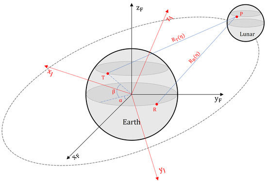
Figure 1. Earth-Centered Earth-Fixed system (ECEF) and geocentric mean equator coordinate system for epoch J2000.0 (geocentric mean J2000 system). ($x_F$, $y_F$, $z_F$) represents ECEF and ($x_J$, $y_J$, $z_J$) represents geocentric mean J2000 system. Point P represents the Moon target, point R and T represent the receiving radar and the transmitting radar, $R_T$($\eta$) and $R_R$($\eta$) represent the slant ranges between SAR and the Moon target at time t = $\eta$.

(1)

Geographic coordinate system, an inertial reference system that describes the position through longitude, latitude and altitude;

(a)

World Geodetic System-1984 (WGS84), giving the longitude, latitude and altitude of the ground-based bistatic SAR;

(b)

Moon geographic coordinate system, giving the longitude, latitude and altitude of the Moon target;

(2)

Fixed coordinate system, an inertial reference system that describes the position with (x, y, z);

(a)

Earth-Centered Earth-Fixed system (ECEF), with the z-axis from the center of the Earth’s mass to the north pole and the x-axis point to the intersection of the prime meridian and the equator;

(b)

Moon-fixed system, with the z-axis from the center of the Moon’s mass to the north pole and the x-axis points to the longitude origin in the equatorial plane;

(3)

Local Cartesian coordinate system, an inertial reference system that describes the position with (x, y, z) centered on the observation point;

The original coordinates of the target point and the two radars will be given in the form of (α, β, h), where $\alpha$, $\beta$ and h are longitude, latitude and altitude.

The coordinates of the ground-based radars can be transformed from (α, β, h) to the fixed coordinate system ($x_E$, $y_E$, $z_E$), using the following formulas

$$x_E=(N+h)cos\left(\beta \right)cos\left(\alpha \right)$$

(1)

$$y_E=(N+h)cos\left(\beta \right)sin\left(\alpha \right)$$

(2)

$$z_E=(N(1-e^2)+h)sin\left(\beta \right)$$

(3)

where N and e are the radius of the curvature in prime vertical and eccentricity of the Earth, given by

$$N=\frac{a}{\sqrt{1-e^{2}si{n}^2\left(\beta \right)}}$$

(4)

$$e=\sqrt{1-\frac{b^2}{a^2}}$$

(5)

where a and b are the semi-major axis and semi-minor axis of the Earth ellipsoid.

Meanwhile, the coordinates of the Moon targets can be transformed from (α, β, h) to the fixed coordinate system ($x_L$, $y_L$, $z_L$) more easily for the reason that the Moon is assumed to be a sphere, which takes the form of

$$x_L=(R+h)cos\left(\beta \right)cos\left(\alpha \right)$$

(6)

$$y_L=(R+h)cos\left(\beta \right)sin\left(\alpha \right)$$

(7)

$$z_L=(R+h)sin\left(\beta \right)$$

(8)

where R is the radius of the Moon.

Then, the transformation matrix of the fixed coordinate system to the geocentric mean J2000 system is fitted with the aid of JPL-DE421 [27]. Because geocentric mean J2000 coordinates vary over time, we fit 3 × 3 transformation matrices, $T_{JF}^E$ and $T_{JF}^L$, for each required moment with the help of ephemeris. Note that the coordinates of the Moon targets are first transformed to the Moon-centric mean equator coordinate system for epoch J2000.0. Consequently, the geocentric mean J2000 coordinates of the Moon’s center of mass need to be added, which takes the form of

$$\left[\begin{array}{c}{x}_E^J\\ y_E^J\\ z_E^J\end{array}\right]=T_{JF}^E\left[\begin{array}{c}{x}_E\\ y_E\\ z_E\end{array}\right]$$

(9)

$$\left[\begin{array}{c}{x}_L^J\\ y_L^J\\ z_L^J\end{array}\right]=T_{JF}^L\left[\begin{array}{c}{x}_L\\ y_L\\ z_L\end{array}\right]+\left[\begin{array}{c}{x}_{LC}^J\\ y_{LC}^J\\ z_{LC}^J\end{array}\right]$$

(10)

where ($x_E^J$, $y_E^J$, $z_E^J$), ($x_L^J$, $y_L^J$, $z_L^J$), ($x_{LC}^J$, $y_{LC}^J$, $z_{LC}^J$) are geocentric mean J2000 coordinates of the ground-based radars, Moon targets and the Moon’s center of mass.

For a more concise representation of the target area grid on the Moon’s surface, the local Cartesian coordinate system is needed, which is a target-centric reference frame, shown in Figure 2. The z-axis coincides with the normal at the target and points in the opposite direction of the Moon’s center of mass and the x-axis points to the east of the Moon in the tangent plane.

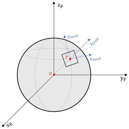
Figure 2. Moon-local Cartesian coordinate system. ($x_F$, $y_F$, $z_F$) represents the Moon-fixed system and ($x_{local}$, $y_{local}$, $z_{local}$) represents the Moon-local Cartesian coordinate system. Point P represents the Moon target and point O represents the Moon’s center of mass.

Moon-centered fixed coordinates ($x_L$, $y_L$, $z_L$) can be transformed to local Cartesian coordinates ($x_{local}$, $y_{local}$, $z_{local}$), using the following matrix

$$T_{local}={\left[\begin{array}{c}XYZ\end{array}\right]}^T$$

(11)

$$X={\left[\begin{array}{c}-sin\left(\alpha \right)cos\left(\alpha \right)0\end{array}\right]}^T$$

(11a)

$$Z=\frac{{\left[x_L{y}_L{z}_L\right]}^T}{\sqrt{x_L^2+y_L^2+z_L^2}}$$

(11b)

$$Y=Z\times X$$

(11c)

3. The Image Resolution of Ground-Based Bistatic SAR

Spatial resolution is the most important performance index of SAR. Bistatic SAR has complex geometry. The definition of range and azimuth direction is more complicated and the resolution calculation is more difficult because of two separate radars. This section refers to the gradient method [28] in order to derive the iso-range resolution and iso-Doppler resolution of the ground-based bistatic SAR.

3.1. Range Resolution

Firstly, we convert the geocentric mean J2000 system to the Moon-local Cartesian coordinate system, so the tangent plane of the Moon’s surface at the target point is equivalent to the ground, which can provide a simpler geometry. Without loss of generality, at time $t=\eta$, the coordinates of transmitting SAR are ($x_T$, $y_T$, $z_T$), the coordinates of the receiving SAR are ($x_R$, $y_R$, $z_R$) and the coordinates of the Moon target are ($x_P$, $y_P$, $z_P$). The two-way slant range is expressed as

$$R_{bi}=\sqrt{{\left(x_P-x_T\right)}^2+{\left(y_P-y_T\right)}^2+{\left(z_P-z_T\right)}^2}+\sqrt{{\left(x_P-x_R\right)}^2+{\left(y_P-y_R\right)}^2+{\left(z_P-z_R\right)}^2}$$

(12)

which can also represent the intersecting line of the ellipsoid and the ground.

In a small area, the curvature of the Moon’s surface can be ignored and the ground is assumed to be flat. The gradient at point ($x_P$, $y_P$) on the intersecting line is given by

$${\mathit{G}}_{\mathit{r}}=\frac{\partial R}{\partial x_P}{\mathit{i}}_{\mathit{x}}+\frac{\partial R}{\partial y_P}{\mathit{i}}_{\mathit{y}}=\left(\frac{x_P-x_T}{R_T}+\frac{x_P-x_R}{R_R}\right){\mathit{i}}_{\mathit{x}}+\left(\frac{y_P-y_T}{R_T}+\frac{y_P-y_R}{R_R}\right){\mathit{i}}_{\mathit{y}}$$

(13)

$$R_T=\sqrt{{\left(x_P-x_T\right)}^2+{\left(y_P-y_T\right)}^2+{\left(z_P-z_T\right)}^2}$$

(13a)

$$R_R=\sqrt{{\left(x_P-x_R\right)}^2+{\left(y_P-y_R\right)}^2+{\left(z_P-z_R\right)}^2}$$

(13b)

The range resolution along the gradient direction is obtained by [29]

$${\rho }_r=\frac{0.886c}{B\left|{\mathit{G}}_{\mathit{r}}\right|}$$

(14)

where c is the speed of light and B is the bandwidth of the signal.

3.2. Doppler Resolution

In order to simplify the formula, we use a vector to express the coordinates and velocity, and give the calculation method of Doppler resolution. According to [28,30], the Doppler frequency is given by

$$f\left(\eta \right)=-\frac{1}{\lambda }\frac{dR\left(\eta \right)}{d\eta }=-\frac{1}{\lambda }\left[\frac{{\mathit{v}}_{\mathit{T}}·({\mathit{r}}_{\mathit{T}}-{\mathit{r}}_{\mathit{P}})}{\left|{\mathit{r}}_{\mathit{T}}-{\mathit{r}}_{\mathit{P}}\right|}-\frac{{\mathit{v}}_{\mathit{R}}·({\mathit{r}}_{\mathit{R}}-{\mathit{r}}_{\mathit{P}})}{\left|{\mathit{r}}_{\mathit{R}}-{\mathit{r}}_{\mathit{P}}\right|}\right]$$

(15)

$$R\left(\eta \right)=\left|{\mathit{r}}_{\mathit{T}}-{\mathit{r}}_{\mathit{P}}\right|+\left|{\mathit{r}}_{\mathit{R}}-{\mathit{r}}_{\mathit{P}}\right|$$

(15a)

where ${\mathit{v}}_{\mathit{T}}$ and ${\mathit{v}}_{\mathit{R}}$ are velocity vectors of the radars, ${\mathit{r}}_{\mathit{P}}$, ${\mathit{r}}_{\mathit{T}}$ and ${\mathit{r}}_{\mathit{R}}$ are position vectors of the Moon target and radars. Note that R$\left(\eta \right)$ is the two-way slant range at time $t=\eta$.

The gradient of the Doppler isoline at point $(x_P,y_P)$ is written as

$${\mathit{G}}_{\mathit{d}}=\frac{\partial f}{\partial x_P}{\mathit{i}}_{\mathit{x}}+\frac{\partial f}{\partial y_P}{\mathit{i}}_{\mathit{y}}=\frac{1}{\lambda }\left[\frac{{\mathit{v}}_{\mathit{Txy}}-\left({\mathit{v}}_{\mathit{T}}·{\mathit{i}}_{\mathit{TP}}\right){\mathit{i}}_{\mathit{TPxy}}}{\left|{\mathit{r}}_{\mathit{T}}-{\mathit{r}}_{\mathit{P}}\right|}+\frac{{\mathit{v}}_{\mathit{Rxy}}-\left({\mathit{v}}_{\mathit{R}}·{\mathit{i}}_{\mathit{RP}}\right){\mathit{i}}_{\mathit{RPxy}}}{\left|{\mathit{r}}_{\mathit{T}}-{\mathit{r}}_{\mathit{P}}\right|}\right]$$

(16)

where ${\mathit{v}}_{\mathit{Txy}}$ and ${\mathit{v}}_{\mathit{Rxy}}$ are projections of ${\mathit{v}}_{\mathit{T}}$ and ${\mathit{v}}_{\mathit{R}}$ on the $(x_P,y_P)$ plane, ${\mathit{i}}_{\mathit{TP}}$ and ${\mathit{i}}_{\mathit{RP}}$ are unit vectors of ${\mathit{r}}_{\mathit{T}}$-${\mathit{v}}_{\mathit{P}}$ and ${\mathit{r}}_{\mathit{R}}$-${\mathit{r}}_{\mathit{P}}$, ${\mathit{i}}_{\mathit{TPxy}}$ and ${\mathit{i}}_{\mathit{RPxy}}$ are projections of ${\mathit{i}}_{\mathit{TP}}$ and ${\mathit{i}}_{\mathit{RP}}$ on the $(x_P,y_P)$ plane.

The Doppler resolution along the gradient direction is obtained by [29]

$${\rho }_d=\frac{0.886}{T_a\left|{\mathit{G}}_{\mathit{d}}\right|}$$

(17)

where $T_a$ is the synthetic aperture time.

3.3. Iso-Range Resolution and Iso-Doppler Resolution

The angle between the range and the Doppler direction of the mono SAR is usually 90°, making the imaging unit rectangular, which ensures the imaging quality [30]. However, unlike the mono SAR, the range direction and Doppler direction of the bistatic SAR are not always vertical. The imaging quality is poor even with high resolution due to the angle between two directions. So, iso-range resolution and iso-Doppler resolution are used.

The Iso-range direction is vertical to the direction of the range gradient ${\mathit{G}}_{\mathit{r}}$ and the Iso-Doppler direction is vertical to the direction of the Doppler gradient ${\mathit{G}}_{\mathit{d}}$. The point target simulation result in Figure 3 shows the iso-range and iso-Doppler directions, which are parallel to the envelope of the result. Therefore, iso-range resolution and iso-Doppler resolution are more suitable for evaluating imaging quality than Doppler resolution and range resolution.

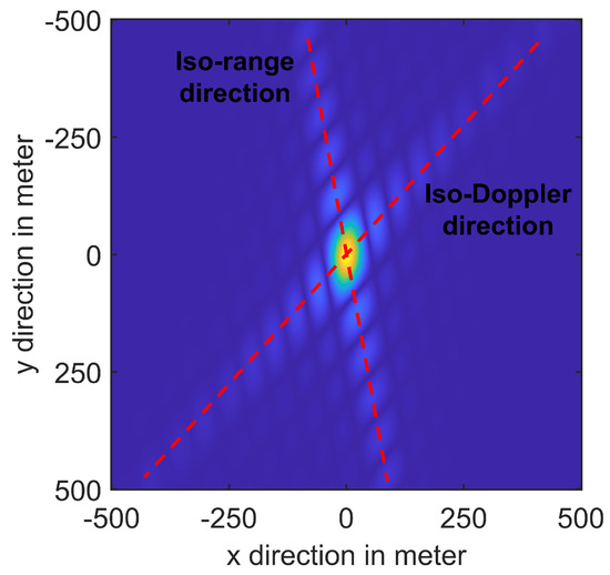
Figure 3. Point target simulation result marked with iso-range and iso-Doppler direction.

$P_{ir}$ is the projection of Doppler gradient in the iso-range direction, which is given by

$$P_{ir}=\frac{{\mathit{G}}_{\mathit{d}}·{\mathit{G}}_{\mathit{r}\perp }}{\left|{\mathit{G}}_{\mathit{r}\perp }\right|}=\frac{x_d{y}_r-x_r{y}_d}{\sqrt{x_r^2+y_r^2}}$$

(18)

where ${\mathit{G}}_{\mathit{d}}=\left(x_d,y_d\right)$ is the Doppler gradient vector, ${\mathit{G}}_{\mathit{r}}=\left(x_r,y_r\right)$ is the range gradient vector and ${\mathit{G}}_{\mathit{r}\perp }$ is the vector vertical to ${\mathit{G}}_{\mathit{r}}$.

In the same way, $P_{id}$ is given by

$$P_{id}=\frac{{\mathit{G}}_{\mathit{r}}·{\mathit{G}}_{\mathit{d}\perp }}{\left|{\mathit{G}}_{\mathit{d}\perp }\right|}=\frac{x_r{y}_d-x_d{y}_r}{\sqrt{x_d^2+y_d^2}}$$

(19)

where ${\mathit{G}}_{\mathit{d}\perp }$ is the vector vertical to ${\mathit{G}}_{\mathit{d}}$.

Then, the iso-range resolution ${\rho }_{ir}$ and the iso-Doppler resolution ${\rho }_{id}$ is obtained by

$${\rho }_{ir}=\frac{0.886}{T_a\left|P_{ir}\right|}$$

(20)

$${\rho }_{id}=\frac{0.886c}{B\left|P_{id}\right|}$$

(21)

We use ${\rho }_{ir}$ to measure Doppler resolution and ${\rho }_{id}$ to measure range resolution in the following sections.

4. The Slant Range of Ground-Based Bistatic SAR

In previous imaging experiments, the calculation of the slant-range has often been simplified, especially for mono SAR, by multiplying a one-way slant-range value by two to estimate the two-way slant range [31].

However, when it comes to ground-based SAR imaging of the Moon, the substantial distance between the Moon and the Earth causes the radars and the target to no longer remain relatively static during the transmission and reception of pulse signals. This renders the ‘stop-and-go’ assumption invalid. With an average distance of 384,000 km between the Moon and the Earth, the interval between signal transmission and reception is approximately 2.5 s, resulting in a position change of the receiving radar exceeding 1 km. Consequently, an accurate calculation method for the slant range becomes imperative. To begin with, a model should be utilized to accurately fit the curved trajectories of the Moon target and the ground-based radars.

4.1. Curve Trajectory Fitting Model

Due to the intricate motion of the Earth and the Moon, which encompasses rotation, revolution, nutation, and precession [32], the conventional models of linear motion and uniform acceleration curve motion fail to accurately depict the trajectories of the target and radars. In order to overcome this limitation, we expand the curve equation to fifth-order polynomials, enabling us to capture the intricate dynamics and complexities involved in the motion.

$$\mathit{L}\left(\eta \right)={\mathit{L}}_{\mathbf{0}}+{\mathit{L}}_{\mathbf{1}}\eta +{\mathit{L}}_{\mathbf{2}}{\eta }^2+{\mathit{L}}_{\mathbf{3}}{\eta }^3+{\mathit{L}}_{\mathbf{4}}{\eta }^4+{\mathit{L}}_{\mathbf{5}}{\eta }^5+O\left({\eta }^6\right)$$

(22)

With the assistance of JPL-DE421, we provide a set of geocentric mean J2000 coordinates for the Moon target and ground-based radars every 3 s over a span of 40 min. Figure 4 illustrates the variation of the fitting residual L2-norm for polynomials of different orders. To enhance the visibility of the changes, we employ a logarithmic coordinate axis. As the polynomial order increases, the residual diminishes rapidly, eventually reaching a plateau after the fifth order. Consequently, the fifth-order polynomial proves to be effective in terms of fitting error.

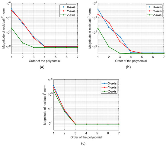
Figure 4. In the order of first to seventh, (a) the residual L2-norm of the polynomial fitting the trajectory of the receiving SAR, (b) the transmitting SAR and (c) the trajectory of the Moon target.

Moreover, we conduct a numerical simulation using the parameters outlined in Table 1 to assess the reliability of the fitting model in Moon imaging. The simulation is based on a central time of 20:11:42 on 31 December 2022, with a synthetic aperture time of 2400 s, fulfilling the resolution requirements of 50 m.

Table 1. Simulation parameters.

Parameter	Symbol	Quantity	Unit
System bandwidth	B	15	MHz
System wavelength	$\lambda$	0.24	m
Emission frequency	f	0.2	MHz
Speed of light	c	299792458	m/s
Position of Moon target	$\mathit{P}$	1.1 W, 8.9 N	degree
Position of transmitting SAR	$\mathit{T}$	80.3 E, 40.6 N	degree
Position of receiving SAR	$\mathit{R}$	106.9 E, 25.7 N	degree
Moon radius	$R_L$	1737400	m
WGS84 Earth radius	$R_E$	6378137	m

Figure 5 depicts the phase errors of polynomials of different orders at each time within the synthetic aperture period. Evidently, when the order exceeds four, the polynomial model adequately satisfies the imaging criteria, and the phase accuracy of the fourth, fifth, sixth, and seventh-order polynomial models appears comparable.

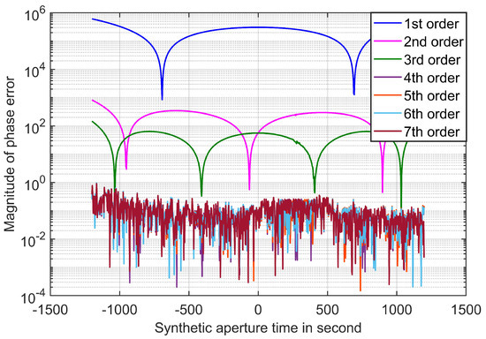
Figure 5. Relationship between the phase error and synthetic aperture time caused by different orders of polynomial model.

The Doppler frequency modulation rate is given by [30]

$$K_a\left(\eta \right)=\frac{1}{\lambda }\frac{d^{2}R\left(\eta \right)}{d{\eta }^2}=\frac{1}{\lambda }\frac{d^2\left(|{\mathit{L}}_{\mathit{T}}\left(\eta \right)-{\mathit{L}}_{\mathit{P}}\left(\eta \right)\left|+|{\mathit{L}}_{\mathit{R}}\left(\eta \right)-{\mathit{L}}_{\mathit{P}}\left(\eta \right)\right|\right)}{d{\eta }^2}$$

(23)

where ${\mathit{L}}_{\mathit{T}}$, ${\mathit{L}}_{\mathit{R}}$ and ${\mathit{L}}_{\mathit{P}}$ are the coordinates of the SARs and the Moon target in the vector form.

Next, we proceed to compare the Doppler frequency and Doppler frequency modulation rate among the fourth, fifth, sixth, and seventh-order polynomial models. Figure 6 highlights part of the result to showcase the distinctions. Over a duration of 2400 s, the Doppler frequency ranges from −9.078 to −521.895, with a maximum difference of 4.978 × 10${}^{-4}$. Meanwhile, the Doppler frequency modulation rate varies between 0.212 and 0.214, with a maximum difference of 4.806 × 10${}^{-6}$. These small errors between these models have minimal impact on the imaging focusing.

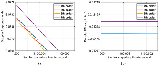
Figure 6. (a) Doppler frequency and (b) Doppler frequency modulation rate of fourth, fifth, sixth and seventh-order polynomial models in a short time.

4.2. Revising ‘Stop-and-Go’ Assumption

According to ‘stop-and-go’ assumption, the two-way slant range of the bistatic SAR is calculated by

$$R_D=R_T\left(\eta \right)+R_R\left(\eta \right)$$

(24)

where $R_T\left(\eta \right)$ and $R_R\left(\eta \right)$ represent the slant ranges between the ground-based radars and the Moon target at time $t=\eta$.

However, the position of the receiving radar undergoes changes as the backscattered signal travels between the Moon and the Earth. To rectify this error, we employ the model depicted in Figure 7. The two-way slant range is approximated by [33]

$$R_D=R_T\left(\eta \right)+R_R\left(\eta +{\tau }_T+{\tau }_R\right)$$

(25)

where ${\tau }_T$ is the time it takes for the transmitted signal to get to the Moon target, which can be calculated accurately by

$$\left|{\mathit{L}}_{\mathit{T}}\left(\eta \right)-{\mathit{L}}_{\mathit{P}}\left(\eta +{\tau }_T\right)\right|=c{\tau }_T$$

(26)

where c is the speed of light, ${\mathit{L}}_{\mathit{T}}$ and ${\mathit{L}}_{\mathit{P}}$ are coordinates of the transmitting SAR and the Moon target in vector form, which are given by

$${\mathit{L}}_{\mathit{T}}\left(\eta \right)={\mathit{L}}_{\mathbf{10}}+{\mathit{L}}_{\mathbf{11}}\eta +{\mathit{L}}_{\mathbf{12}}{\eta }^2+{\mathit{L}}_{\mathbf{13}}{\eta }^3+{\mathit{L}}_{\mathbf{14}}{\eta }^4+{\mathit{L}}_{\mathbf{15}}{\eta }^5$$

(26a)

$$\begin{array}{cc}\hfill {\mathit{L}}_{\mathit{P}}\left(\eta +{\tau }_T\right)& ={\mathit{L}}_{\mathbf{20}}+{\mathit{L}}_{\mathbf{21}}\left(\eta +{\tau }_T\right)+{\mathit{L}}_{\mathbf{22}}{\left(\eta +{\tau }_T\right)}^2+{\mathit{L}}_{\mathbf{23}}{\left(\eta +{\tau }_T\right)}^3\hfill \\ \hfill & +{\mathit{L}}_{\mathbf{24}}{\left(\eta +{\tau }_T\right)}^4+{\mathit{L}}_{\mathbf{25}}{\left(\eta +{\tau }_T\right)}^5\hfill \end{array}$$

(26b)

${\tau }_R$ is the received time of the backscattered signal, which can be calculated by

$$\left|{\mathit{L}}_{\mathit{R}}(\eta +{\tau }_T+{\tau }_R)-{\mathit{L}}_{\mathit{P}}\left(\eta +{\tau }_T\right)\right|=c{\tau }_R$$

(27)

where ${\mathit{L}}_{\mathit{R}}$ is the coordinate of the receiving SAR, which is given by

$$\begin{array}{cc}\hfill {\mathit{L}}_{\mathit{P}}\left(\eta +{\tau }_T+{\tau }_R\right)& ={\mathit{L}}_{\mathbf{30}}+{\mathit{L}}_{\mathbf{31}}\left(\eta +{\tau }_T+{\tau }_R\right)+{\mathit{L}}_{\mathbf{32}}{\left(\eta +{\tau }_T+{\tau }_R\right)}^2+{\mathit{L}}_{\mathbf{33}}{\left(\eta +{\tau }_T+{\tau }_R\right)}^3\hfill \\ \hfill & +{\mathit{L}}_{\mathbf{34}}{\left(\eta +{\tau }_T+{\tau }_R\right)}^4+{\mathit{L}}_{\mathbf{35}}{\left(\eta +{\tau }_T+{\tau }_R\right)}^5\hfill \end{array}$$

(27a)

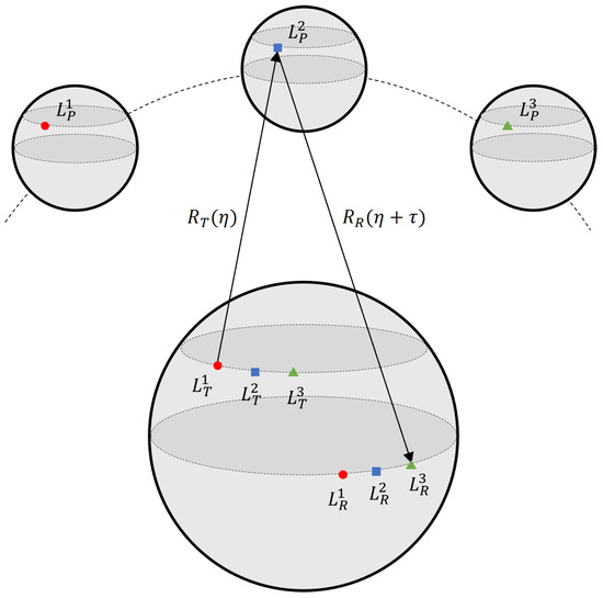
Figure 7. Transceiver separation slant-range model. ${\mathit{L}}_{\mathit{T}}^{\mathit{n}}$, ${\mathit{L}}_{\mathit{R}}^{\mathit{n}}$ and ${\mathit{L}}_{\mathit{P}}^{\mathit{n}}$ represent coordinates of transmitting SAR, receiving SAR and Moon target at different time n.

Then, the two-way slant range can be expressed as

$$R_D=c\left({\tau }_T+{\tau }_R\right)$$

(28)

This calculation method for the slant range yields an accurate solution for high-order equations without resorting to mathematical approximations. Moreover, during the derivation of the two-way slant range, the motion trajectories are not simplified or constrained; instead, they are fitted with high-order polynomials. As a result, the slant range obtained through this method is more precise.

4.3. Changes in Imaging Quality

According to the transceiver separation slant-range model, $R_T$ and $R_R$ are expressed as

$$R_T\left(\eta \right)=\left|{\mathit{L}}_{\mathit{T}}\left(\eta \right)-{\mathit{L}}_{\mathit{P}}\left(\eta +{\tau }_T\right)\right|$$

(29)

$$R_R\left(\eta \right)=\left|{\mathit{L}}_{\mathit{R}}\left(\eta +{\tau }_T+{\tau }_R\right)-{\mathit{L}}_{\mathit{P}}\left(\eta +{\tau }_T\right)\right|$$

(30)

The two-way delay is

$$\tau =\frac{R_T\left(\eta \right)+R_R\left(\eta \right)}{c}$$

(31)

Compared to the ‘stop-and-go’ assumption, the transceiver separation slant-range model offers greater accuracy. To illustrate the disparity between them, we conducted simulations using the parameters listed in Table 1. In Figure 8, we observe that the ‘stop-and-go’ assumption introduces a small two-way delay error. Within the synthetic aperture time, the maximum error exceeds $1.1\times {10}^{-7}$, which is substantial enough to cause image shift when employing the BP algorithm with a bandwidth of 15 MHz. Additionally, the variation in the Doppler frequency and Doppler frequency modulation rate is not significant, indicating that the ‘stop-and-go’ assumption has minimal impact on the resolution calculation.

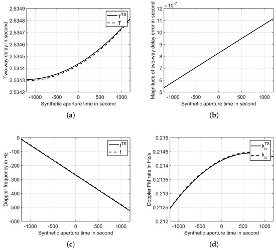
Figure 8. Variation between the transceiver separation slant-range model and the model with ‘stop-and-go’ assumption. (a) two-way delay; (b) magnitude of two-way delay error; (c) Doppler frequency; (d) Doppler frequency modulation rate. The superscript $TS$ represents the transceiver separation slant-range model.

To further investigate the influence of the ‘stop-and-go’ assumption on resolution calculations, we computed the resolution of the target point using different slant-range models over a 2400-s interval centered at 20:11:42. Figure 9 illustrates the iso-doppler and iso-range resolutions at each time point. The ‘stop-and-go’ assumption has minimal impact on these resolutions due to the small errors in slant range and vector, which are insignificant compared to the distance between the Earth and the Moon. Consequently, the gradients of the range and Doppler, as described by Equations (13) and (16), remain almost unchanged.

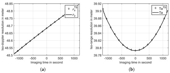
Figure 9. (a) Iso-Doppler resolution and (b) iso-range resolution of different slant-range models at each time. Note that the synthetic aperture time is set to 2400 s when we calculate the iso-range resolution.

5. Imaging Ability Analysis of Ground-Based Bistatic SAR

In this section, we present a comprehensive analysis of the imaging capabilities of ground-based bistatic SAR for Moon imaging. We begin by analyzing the effective imaging time of the system. Although the orbital period of the Moon is 27.32166 days, it is important to consider the radar’s look angles and the angle between the iso-range gradient and iso-Doppler gradient, as these factors restrict the ability to image the Moon continuously. Next, we investigate the imaging resolution of targets located at various positions on the Moon’s surface within effective imaging time.

5.1. Effective Imaging Time Analysis

To determine whether a Moon imaging experiment can be conducted at a specific time, two conditions must be validated. The first condition pertains to signal accessibility, which ensures that the transmitted signal can reach the target position and the reflected signal can be received by FAST. Figure 10 illustrates the vector relationship between the transmitting and receiving signal paths, along with the definition of four vector angles. Signal accessibility necessitates that all four angles satisfy the following condition:

$${\theta }_1<{\gamma }_T,{\theta }_2<{\gamma }_R,{\theta }_3<90°,{\theta }_4<90°$$

(32)

where ${\gamma }_T$ and ${\gamma }_R$ represent the maximum look angles of the transmitting radar and the receiving radar.

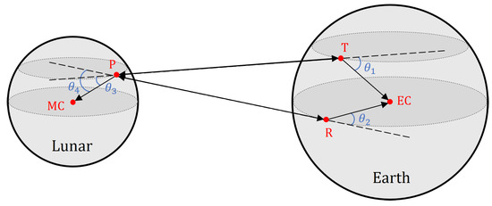
Figure 10. Vector analysis of signal accessibility. EC and MC represent the Earth’s center of mass and the Moon’s center of mass. ${\theta }_1$, ${\theta }_2$, ${\theta }_3$ and ${\theta }_4$ represent the vector angles.

The second condition pertains to ensuring the quality of the imaging. Bistatic SAR imaging differs from monostatic SAR imaging due to the utilization of separate transmitting and receiving radars, resulting in more intricate ground resolution characteristics. Unlike monostatic SAR, the iso-range direction and iso-Doppler direction in bistatic SAR imaging are not necessarily perpendicular to each other. When the angle between these two directions is either too small or too large, the desired imaging effect cannot be achieved. Therefore, it is crucial to select an imaging moment when the angle is close to 90° in order to attain optimal imaging results.

Using the parameters provided in Table 1 and Table 2, we conducted simulations to determine the effective imaging time for ground-based bistatic SAR between 8 November and 7 December 2022. The simulation results indicate that within these 30 days, the effective imaging time amounts to 878,241 s (equivalent to 10.16 days). Figure 11a,b illustrate that the iso-range direction remains relatively stable, changing within 20° during short time intervals. However, the iso-Doppler direction exhibits significant fluctuations, with a maximum difference of 90°. Consequently, the angle between the iso-range direction and the iso-Doppler direction undergoes sharp changes in Figure 11c, rendering certain time periods unsuitable for imaging, even if the Moon target is observable.

Table 2. Simulation parameters-2.

Parameter	Symbol	Quantity	Unit
Look angle of transmitting SAR	${\gamma }_T$	$\pm 90$	degree
Look angle of receiving SAR	${\gamma }_R$	$\pm 90$	degree
Angle between two direction	$\varphi$	60–120	degree
Synthetic aperture time	$T_a$	2400	second

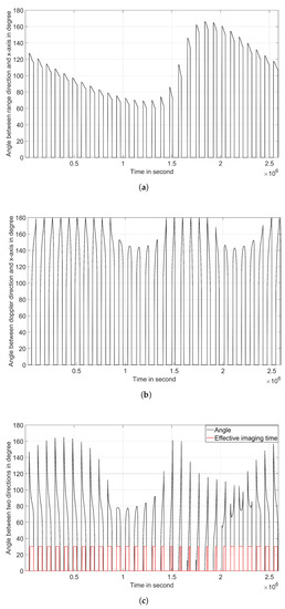
Figure 11. Changes of (a) range direction and (b) Doppler direction. (c) Changes of angle between two directions and effective imaging time.

During the simulation, we did not impose any restrictions on the radar’s look angle and had lenient requirements for the angle between the iso-range direction and the iso-Doppler direction. However, it is important to note that if the look angles of the radars are constrained or higher imaging quality is desired, the effective imaging time will be reduced.

5.2. Imaging Resolution Analysis

After determining the effective imaging time, it becomes necessary to analyze the iso-range resolution and iso-Doppler resolution of the target point. The two-dimensional resolution of the same target varies at different times, and imaging different targets at the same time also yields varying two-dimensional resolutions.

To begin, we select a fixed target point and examine the changes in two-dimensional resolution over a period. Utilizing the parameters provided in Table 1 and Table 2, we simulate the change of two-dimensional resolution of a target point at (8.9°N, 1.1°W), which is near the center of the Moon disk.

Figure 12a,b depict the alterations in iso-Doppler resolution over the course of a 30-day period. The changes in iso-Doppler resolution during each short period of effective imaging time are generally small, typically less than 1 m. However, the iso-Doppler resolution exhibits significant variations across different effective time periods, indicating differences of over 150 m when observing the same target point on different days.

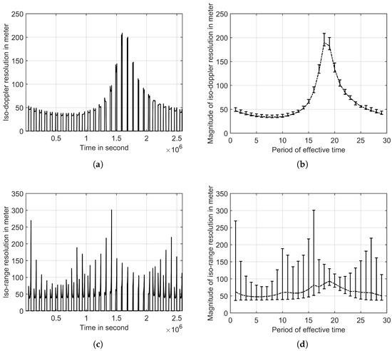
Figure 12. Changes of (a,b) iso-Doppler resolution and (c,d) iso-range resolution. (b,d) shows the mean, minimum and maximum resolutions for each effective time period.

Figure 12c,d showcase the variation in iso-range resolution. In contrast to the iso-Doppler resolution, the iso-range resolution demonstrates significant fluctuations within each effective time period, over 100 m even within the span of a single day. However, the performance of iso-range resolution is similar across different effective time periods.

Therefore, in the actual imaging experiment, it becomes crucial to choose the appropriate time window based on the iso-Doppler resolution. Subsequently, within this effective time period, the optimal imaging time is selected based on the iso-range resolution.

Secondly, the influence of the longitude and latitude of the Moon target on the imaging resolution is studied. We select 25 Moon targets with a latitude of $-60°$, $-30°$, 0°, 30°, 60° and longitude of $-60°$, $-30°$, 0°, 30°, 60° to calculate the mean value of iso-Doppler resolution and iso-range resolution in the effective time. The theoretically calculated resolutions are listed in Table 3 and Table 4.

Table 3. Mean iso-Doppler resolution of simulation.

	Longitude	$-60°$	$-30°$	0°	30°	60°
Latitude
$-60°$		9.42 m	10.34 m	10.81 m	10.25 m	9.46 m
$-30°$		10.52 m	14.99 m	19.95 m	14.32 m	10.38 m
0°		10.70 m	17.57 m	84.52 m	20.09 m	10.98 m
30°		9.88 m	13.29 m	18.27 m	12.84 m	9.89 m
60°		9.31 m	10.07 m	10.53 m	10.02 m	9.30 m

Table 4. Mean iso-range resolution of simulation.

	Longitude	$-60°$	$-30°$	0°	30°	60°
Latitude
$-60°$		88.73 m	73.09 m	69.28 m	71.21 m	80.22 m
$-30°$		81.42 m	68.63 m	67.05 m	63.91 m	70.65 m
0°		87.31 m	77.14 m	59.16 m	87.78 m	88.03 m
30°		70.99 m	63.78 m	61.29 m	66.52 m	76.66 m
60°		81.35 m	71.29 m	68.88 m	70.11 m	76.55 m

From the results in Table 3, we can find that, with the increase of longitude and latitude, iso-Doppler resolution improves. Figure 13a shows the distance contour on the surface of the Moon. Due to the movement of the Moon and the Earth, the sub-radar points of transmitting SAR and receiving SAR move periodically between $\pm 10°$ longitude and $\pm 10°$ latitude. The distribution of distance contour is dense far from the sub-radar points and sparse near it, which means as the distance to the sub-radar points increases, ${\mathit{G}}_{\mathit{r}}$ increases, $P_{id}$ increases and iso-Doppler resolution ${\rho }_{\mathit{id}}$ improves.

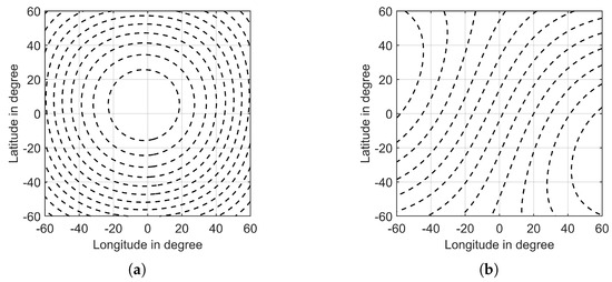
Figure 13. (a) Distance contour and (b) Doppler frequency contour on the Moon’s surface. They cover the area of 60°W to 60°E and 60°N to 60°S, including most of the visible region of the Moon.

Figure 13b shows the Doppler frequency contour on the surface of the Moon. The distribution of Doppler frequency contour with position is opposite to that of distance contour, but the change is much smaller. So, at the edge of the Moon disk, ${\mathit{G}}_{\mathit{d}}$ decreases, $P_{ir}$ decreases and iso-range resolution ${\rho }_{\mathit{ir}}$ becomes worse. The results in Table 4 reflect the trend.

5.3. Point Targets Simulation

Due to the symmetry of the Moon, we have chosen nine target points with a longitude of 0°, 30°, 60° and a latitude of 0°, 30°, 60° to carry out the point targets simulation, generating images using the BP algorithm. Then, we measure the iso-Doppler resolution and iso-range resolution, comparing them to the results obtained through theoretical calculation. The central time is set at 3:37:45 on 19 November 2022. From Figure 14, Table 5 and Table 6, it is evident that the resolutions achieved through point target simulations are in line with the theoretically calculated values. This outcome serves as a validation of the accuracy and reliability of both the imaging model and the resolution analysis method.

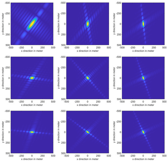
Figure 14. The points simulation results of different positions on the Moon’s surface. The latitude values are 0°, 30°, 60° from top to bottom and the longitude values are 0°, 30°, 60° from left to right. Note that we set $B=5$ MHz, $T_a=2400$ s to make iso-range resolution and iso-Doppler resolution close.

Table 5. Iso-range resolution of theoretical calculation and point target simulation.

Latitude	Longitude	Theoretical Calculation	Point Target Simulation	Relative Error
0°	0°	55.134	55.179	0.081%
0°	30°	77.402	77.487	0.109%
0°	60°	86.438	86.514	0.088%
30°	0°	63.642	63.723	0.127%
30°	30°	55.318	55.391	0.132%
30°	60°	58.356	58.437	0.138%
60°	0°	66.895	66.965	0.105%
60°	30°	58.604	58.688	0.143%
60°	60°	56.139	56.154	0.025%

Table 6. Iso-Doppler resolution of theoretical calculation and point target simulation.

Latitude	Longitude	Theoretical Calculation	Point Target Simulation	Relative Error
0°	0°	199.285	198.423	0.434%
0°	30°	58.820	58.945	0.212%
0°	60°	32.787	32.712	0.229%
30°	0°	49.360	49.179	0.369%
30°	30°	35.109	35.192	0.237%
30°	60°	28.103	28.186	0.294%
60°	0°	30.088	30.178	0.298%
60°	30°	28.156	28.193	0.131%
60°	60°	26.753	26.831	0.290%

6. Conclusions

For Moon imaging missions using ground-based bistatic SAR systems such as FAST and other active radars, the iso-Doppler and iso-range resolutions of different observation areas exhibit significant differences at a given imaging time. Additionally, within a given observation area, the iso-Doppler and iso-range resolutions vary significantly with different imaging times. Hence, it becomes crucial to establish the relationship between resolution capabilities, radar systems, and observation conditions to ensure the success of Moon imaging missions. This paper introduces a methodology for analyzing the Moon imaging capabilities of FAST in bistatic configurations along with other radars. The proposed method allows us to predict imaging resolutions in advance and set appropriate parameters based on resolution requirements, such as bandwidth, synthetic aperture time, imaging time period, observation location, and more. This paper offers theoretical guidance for Moon imaging missions using FAST in bistatic configurations, and the approach can also be extended to missions involving imaging other celestial bodies or signal station configurations.

References

- Pettengill, G.H.; Henry, J.C. Enhancement of radar reflectivity associated with the Moon Crater tycho. J. Geophys. Res. 1962, 67, 4881–4885. [Google Scholar] [CrossRef]
- Thompson, T.W. Map of Moon radar reflectivity at 7.5-m wavelength. Icarus 1970, 13, 363–370. [Google Scholar] [CrossRef]
- Thompson, T.W. Atlas of Moon radar maps at 70-cm wavelength. Moon 1974, 10, 51–85. [Google Scholar] [CrossRef]
- Zisk, S.H.; Pettengill, G.H.; Catuna, G.W. High-resolution radar maps of the Moon’s surface at 3.8-cm wavelength. Moon 1974, 10, 17–50. [Google Scholar] [CrossRef]
- Thompson, T.W. High-resolution Moon radar map at 70-cm wavelength. Earth Moon Planets 1987, 37, 59–70. [Google Scholar] [CrossRef]
- Stacy, N.J.S. High-Resolution Synthetic Aperture Radar Observations of the Moon. Ph.D. Thesis, Cornell University, Ithaca, NY, USA, May 1993. [Google Scholar]
- Stacy, N.J.S.; Campbell, D.B.; Ford, P.G. Arecibo radar mapping of the Moon poles: A search for ice deposits. Science 1997, 276, 1527–1530. [Google Scholar] [CrossRef]
- Campbell, B.A.; Campbell, D.B.; Margot, J.L.; Ghent, R.R.; Nolan, M.; Chandler, J.; Carter, L.M.; Stacy, N.J.S. Focused 70-cm wavelength radar mapping of the Moon. IEEE Trans. Geosci. Remote Sens. 2007, 45, 4032–4042. [Google Scholar] [CrossRef]
- Campbell, B.A.; Hawke, B.R.; Morgan, G.A.; Carter, L.M.; Campbell, D.B.; Nolan, M. Improved discrimination of volcanic complexes, tectonic features, and regolith properties in mare serenitatis from Earth-based radar mapping. J. Geophys. Res. Planets 2014, 119, 313–330. [Google Scholar] [CrossRef]
- Vierinen, J.; Lehtinen, M.S. 32-cm wavelength radar mapping of the Moon. In Proceedings of the 2009 European Radar Conference (EuRAD), Rome, Italy, 30 September–2 October 2009; IEEE: New York, NY, USA, 2009; pp. 222–225. [Google Scholar]
- Vierinen, J.; Tveito, T.; Gustavsson, B.; Kesaraju, S.; Milla, M. Radar images of the Moon at 6-meter wavelength. Icarus 2017, 297, 179–188. [Google Scholar] [CrossRef]
- Taylor, P. Next Generation Planetary Radar with the Green Bank Telescope. Am. Astron. Soc. Meet. Abstr. 2023, 55, 139. [Google Scholar]
- Harmon, J.K.; Nolan, M.C.; Husmann, D.I.; Campbell, B.A. Arecibo radar imagery of Mars: The major volcanic provinces. Icarus 2012, 220, 990–1030. [Google Scholar] [CrossRef]
- Neish, C.D.; Blewett, D.T.; Harmon, J.K.; Coman, E.I.; Cahill, J.T.S.; Ernst, C.M. A comparison of rayed craters on the Moon and Mercury. J. Geophys. Res. Planets 2013, 113, 2247–2261. [Google Scholar] [CrossRef]
- Lawrence, K.J.; Benner, L.A.M.; Brozovic, M.; Ostro, S.J.; Jao, J.S.; Giorgini, J.D.; Slade, M.A.; Jurgens, R.F.; Nolan, M.C.; Howell, E.S.; et al. Arecibo and goldstone radar images of near-Earth asteroid (469896) 2005 WC1. Icarus 2018, 300, 12–20. [Google Scholar] [CrossRef]
- Xu, Z.; Chen, K. On signal modeling of Moon-based Synthetic Aperture Radar (SAR) imaging of Earth. Remote Sens. 2018, 10, 486. [Google Scholar] [CrossRef]
- Xu, Z.; Chen, K.; Zhou, G. Effects of the Earth’s irregular rotation on the Moon-based synthetic aperture radar imaging. IEEE Access 2019, 99, 155014–155027. [Google Scholar] [CrossRef]
- Huang, J.; Guo, H.; Liu, G.; Shen, G.; Ye, H.; Deng, Y.; Dong, R. Spatio-temporal characteristics for Moon-based Earth observations. Remote Sens. 2020, 12, 2848. [Google Scholar] [CrossRef]
- Vaishnav, R.; Jin, Y.; Mostafa, M.G.; Aziz, S.R.; Zhang, S.; Jacobi, C. Study of the upper transition height using ISR observations and IRI predictions over Arecibo. Adv. Space Res. 2021, 68, 2177–2185. [Google Scholar] [CrossRef]
- Wu, K.; Ji, C.; Luo, L.; Wang, X. Simulation Study of Moon-Based InSAR Observation for Solid Earth Tides. Remote Sens. 2020, 12, 123. [Google Scholar] [CrossRef]
- Zhang, K.; Wu, J.; Li, D.; Krčo, M.; Staveley-Smith, L.; Tang, N.; Qian, L.; Liu, M.; Jin, C.; Yue, Y.; et al. Status and perspectives of the CRAFTS extra-galactic HI survey. Sci. China Phys. Mech. Astron. 2019, 62, 1–9. [Google Scholar] [CrossRef]
- Nan, R. Five hundred meter aperture spherical radio telescope (FAST). Sci. China Ser. G 2006, 49, 129–148. [Google Scholar] [CrossRef]
- Yan, J.; Zhang, H. Introduction to main application goals of Five-hundred-meter Aperture Spherical radio Telescope. J. Deep Space Explor. 2020, 7, 128–135. [Google Scholar]
- Li, M.; Yue, X.; Wang, Y.; Wang, J.; Ding, F.; Vierinen, J.; Zhang, N.; Wang, Z.; Ning, B.; Zhao, B.; et al. Moon imaging technique and experiments based on Sanya incoherent scatter radar. IEEE Trans. Geosci. Remote Sens. 2022, 60, 1–14. [Google Scholar] [CrossRef]
- Schuh, H.; Behrend, D. VLBI: A fascinating technique for geodesy and astrometry. J. Geodyn. 2012, 61, 68–80. [Google Scholar] [CrossRef]
- Chen, R.; Zhang, H.; Jin, C.; Gao, Z.; Zhu, Y.; Zhu, K.; Jiang, P.; Yue, Y.-L.; Lu, J.-G.; Zhang, B.; et al. FAST VLBI: Current status and future plans. Res. Astron. Astrophys. 2020, 20, 74. [Google Scholar] [CrossRef]
- Folkner, W.M.; Williams, J.G.; Boggs, D.H. The planetary and lunar ephemeris DE 421. IPN Prog. Rep. 2009, 42, 1. [Google Scholar]
- Qiu, X.; Hu, D.; Ding, C. The resolution ability and velocity determination in translational variant bistatic SAR. J. Astronaut. 2009, 20, 1609–1614. [Google Scholar]
- Cardillo, G.P. On the use of the gradient to determine bistatic SAR resolution. In International Symposium on Antennas and Propagation Society, Merging Technologies for the 90’s; IEEE: New York, NY, USA, 1990; pp. 1032–1035. [Google Scholar]
- Cumming, I.G.; Wong, F.H. Digital Signal Processing of Synthetic Aperture Radar Data: Algorithms and Implementation; Artech House: Norwood, MA, USA, 2005. [Google Scholar]
- Li, M.; Yue, X.; Ding, F.; Ning, B.; Wang, J.; Zhang, N.; Luo, J.; Huang, L.; Wang, Y.; Wang, Z. Focused Moon imaging experiment using the back projection algorithm based on Sanya incoherent scatter radar. Remote Sens. 2022, 14, 2048. [Google Scholar] [CrossRef]
- Ouyang, Z.Y. Introduction to Moon Science, 1st ed.; China Astron Publishing House: Beijing, China, 2005. [Google Scholar]
- Hu, C.; Long, T.; Zeng, T.; Liu, F.; Liu, Z. The accurate focusing and resolution analysis method in geosynchronous SAR. IEEE Trans. Geosci. Remote Sens. 2011, 49, 3548–3563. [Google Scholar] [CrossRef]
Disclaimer/Publisher’s Note: The statements, opinions and data contained in all publications are solely those of the individual author(s) and contributor(s) and not of MDPI and/or the editor(s). MDPI and/or the editor(s) disclaim responsibility for any injury to people or property resulting from any ideas, methods, instructions or products referred to in the content. |
© 2023 by the authors. Licensee MDPI, Basel, Switzerland. This article is an open access article distributed under the terms and conditions of the Creative Commons Attribution (CC BY) license (https://creativecommons.org/licenses/by/4.0/).