Abstract
Global mapping of essential vegetation traits (EVTs) through data acquired by Earth-observing satellites provides a spatially explicit way to analyze the current vegetation states and dynamics of our planet. Although significant efforts have been made, there is still a lack of global and consistently derived multi-temporal trait maps that are cloud-free. Here we present the processing chain for the spatiotemporally continuous production of four EVTs at a global scale: (1) fraction of absorbed photosynthetically active radiation (FAPAR), (2) leaf area index (LAI), (3) fractional vegetation cover (FVC), and (4) leaf chlorophyll content (LCC). The proposed workflow presents a scalable processing approach to the global cloud-free mapping of the EVTs. Hybrid retrieval models, named S3-TOA-GPR-1.0-WS, were implemented into Google Earth Engine (GEE) using Sentinel-3 Ocean and Land Color Instrument (OLCI) Level-1B for the mapping of the four EVTs along with associated uncertainty estimates. We used the Whittaker smoother (WS) for the temporal reconstruction of the four EVTs, which led to continuous data streams, here applied to the year 2019. Cloud-free maps were produced at 5 km spatial resolution at 10-day time intervals. The consistency and plausibility of the EVT estimates for the resulting annual profiles were evaluated by per-pixel intra-annually correlating against corresponding vegetation products of both MODIS and Copernicus Global Land Service (CGLS). The most consistent results were obtained for LAI, which showed intra-annual correlations with an average Pearson correlation coefficient (R) of 0.57 against the CGLS LAI product. Globally, the EVT products showed consistent results, specifically obtaining higher correlation than 0.5 with reference products between 30 and 60° latitude in the Northern Hemisphere. Additionally, intra-annual goodness-of-fit statistics were also calculated locally against reference products over four distinct vegetated land covers. As a general trend, vegetated land covers with pronounced phenological dynamics led to high correlations between the different products. However, sparsely vegetated fields as well as areas near the equator linked to smaller seasonality led to lower correlations. We conclude that the global gap-free mapping of the four EVTs was overall consistent. Thanks to GEE, the entire OLCI L1B catalogue can be processed efficiently into the EVT products on a global scale and made cloud-free with the WS temporal reconstruction method. Additionally, GEE facilitates the workflow to be operationally applicable and easily accessible to the broader community.
1. Introduction
Through a fleet of Earth observation (EO) satellites, Europe is dedicated to keeping track of the dynamics of the global vegetation cover [1]. Among the most innovative vegetation monitoring concepts is the FLuorescence EXplorer (FLEX), which was selected as ESA’s eighth Earth Explorer (EE8). Foreseen to be launched in 2025, FLEX will orbit in tandem 100 km ahead of a Copernicus Sentinel-3 (S3) satellite, and will globally measure the full spectral emission of solar-induced chlorophyll fluorescence (SIF) from terrestrial vegetation. The FLEX-S3 tandem mission will offer unprecedented possibilities to increase knowledge of the basic functioning of the Earth’s vegetation, notably the photosynthetic process of plants resulting in carbon fixation [2]. In support of interpreting the spectrally resolved SIF towards the quantification of photosynthetic activity, essential vegetation traits (EVTs) will be derived from the principal optical sensors, i.e., S3 Ocean and Land Color Instrument (OLCI) and FLEX Fluorescence Imaging Spectrometer (FLORIS). These EVTs include (1) fraction of absorbed photosynthetically active radiation (FAPAR), (2) leaf area index (LAI), (3) fractional vegetation cover (FVC), and (4) leaf chlorophyll content (LCC). As opposed to vegetation indices, which are relative measures, EVTs are quantifiable variables with physical units and can be collected during field campaigns. The four targeted EVTs are briefly described as follows.
FAPAR refers to the amount of incoming solar radiation absorbed by living green vegetation in the spectral range of 400–700 nm, divided by the total amount of radiation absorbed at the surface [3,4]. Overall, FAPAR is an important variable used for modelling primary productivity [5]. In addition, FAPAR provides an observational constraint for simulating vegetation–atmosphere carbon fluxes in terrestrial biosphere models [4,6].
LAI is defined as half of the total intercepting leaf area per unit ground surface area [7]. The variable is strongly related to canopy photosynthesis and evapotranspiration [5] and plays an essential role in the exchange of energy and water between the biosphere and atmosphere. Hence, LAI can be seen as a key component of biogeochemical cycles in ecosystems [8]. FVC corresponds to the fraction of green vegetation as seen from nadir, and reflects the spatial extent of photosynthetic leaf areas [9]. Generally, FVC is an important biophysical indicator required for modelling land surface processes, climate change, and numerical weather prediction [10]. The amount of solar radiation absorbed by leaves is driven by photosynthetic pigments, with chlorophyll a and b as the most abundant ones. LCC directly determines photosynthetic potential and thus primary production [11,12].
Whereas FLEX is set to be launched in 2025, S3 has been in orbit since 2016 (S3-A) and 2018 (S3-B), and two more additional satellites are planned to be launched in 2023 (S3-C) and 2025 (S3-D). The S3 mission originated from the need to provide data continuity for ERS, ENVISAT, and SPOT-VGT satellites. ESA has supported several activities to retrieve EVTs from data acquired by the OLCI sensor onboard S3 [13,14]. The OLCI instrument onboard Sentinel-3 is advantageous for EVT retrieval at the continental or global scale given a spatial resolution of 300 m with worldwide coverage every ∼2 days and its spectral range from 400 to 1040 nm [15]. For instance, the red and red-edge bands (bands O8 to O12) are especially important for chlorophyll monitoring and a crucial indicator of plant health [16]. Operational retrieval algorithms targeting these EVTs have been presented within the context of supporting the FLEX mission. A prototyping approach was provided by De Grave et al. [17] with the concept of hybrid retrieval approaches. Hybrid models combine the generalization capabilities offered by radiative transfer models (RTMs) with the flexibility and computational efficiency of machine learning regression algorithms [18]. In this sense, De Grave et al. [17] used the RTM Soil Canopy Observation, Photochemistry and Energy fluxes (SCOPE) [19] to generate a database of reflectance spectra corresponding to a large variety of canopy states. Subsequently, the dataset served as input to train a Gaussian processes regression (GPR) algorithm and establish individual models for the targeted variables given all available bands, i.e., coming from OLCI or FLORIS or their synergy. While these hybrid models served for the first processing of S3-OLCI top-of-canopy (TOC) reflectance images, they were not implemented into an operational processing chain. Yet, when it comes to processing at a continental scale, computationally efficient solutions have to be sought. Moreover, essential preprocessing steps, such as selecting and preparing S3 tiles from the Copernicus data hub, add up to computation time. In addition, imposed restrictions on the data hub can be a substantial bottleneck even for fully automated processes. Consequently, to achieve dynamic processing of a vast amount of S3 data, there is the need to migrate towards cloud-computing platforms. Taking advantage of the Google Earth Engine (GEE) facilities, recent studies demonstrated that GPR models can be integrated into the GEE framework [20,21,22], thus enabling conversion of the GEE satellite catalogue into vegetation properties. However, a key challenge with GEE is that only top-of-atmosphere (TOA) L1B radiance data are provided by the platform. This implied that the hybrid GPR models needed to be upscaled from TOC reflectance to TOA radiance data, thereby taking atmospheric effects into account. Advancing along this line, Reyes-Muñoz et al. [23] presented a worflow for the processing of the four EVTs based on the TOA S3-OLCI collection available in the GEE platform. To do so, the SCOPE-simulated reflectance was coupled with simulations coming from the atmospheric RTM Second Simulation of a Satellite Signal in the Solar Spectrum-vector (6SV) [24]. The subsequently trained retrieval algorithms, named “S3-TOA-GPR-1.0” models, were then implemented in GEE to enable large-scale quantification of the traits from TOA data as acquired by the S3-OLCI sensor. Thanks to the unparalleled processing capacity of GEE, the first spatiotemporal maps were presented and validated at the European continental scale [23]. This has opened up opportunities to process data on a global scale and to provide spatially and temporally continuous data streams. Nonetheless, it has yet to be determined if the S3-TOA-GPR-1.0 EVT models are viable for global use and can operate throughout the year, which is required to confirm their suitability for operational use within the FLEX processing chain. When upscaling towards global processing, the availability of continuous EO data streams is often hampered by cloud cover. Omnipresent cloud layers are prevalent in many regions of the world. In such situations, it may not be possible to obtain a cloud-free image for several weeks or even months [25,26]. Furthermore, additional inadequate weather conditions (e.g., snow, dust, aerosols) [27], instrumentation changes or errors [28], and low temporal resolution of the sensors [29] can induce inconsistencies in the continuity of data streams. Still, clouds and their shadows are probably the most stringent limitation of optical satellite data, since the majority of Earth’s terrestrial surface is regularly covered by clouds. Therefore, spatiotemporal reconstruction of cloud-free satellite imagery methods became a crucial step in EO data processing. Time series reconstruction algorithms further can be broadly categorized into (1) smoothing and empirical methods, (2) data transformations, and (3) curve-fitting methods [30]. Among these, two main groups can be identified [31], those being decomposition techniques, which are typically applied to whole time series, and curve-fitting methods focusing on a limited temporal window. Curve-fitting methods are conventionally used, with Fourier-based approaches, double logistic curves, and the Savitzky–Golay filter (SGF) as the most popular methods for the reconstruction of EO data [25,32]. To overcome identified disadvantages of these smoothers, extended versions of the Whittaker Smoother (WS) [33] have been introduced by Eilers [34], Atzberger and Eilers [35].
The WS function, which is based on penalized least squares, fits a discrete series to discrete data and balances the reliability of the observations with the roughness of the smoothed curve. In particular, the smoother allows continuous control over smoothness, works fast, and is capable of automatic interpolation [35]. Comparison analysis of these methods for reconstructing time series purposes often found the WS among the top-performing [36,37,38,39], although the success of a method may also depend on the nature of the input data [40]. Thanks to its computational efficiency and flexibility, the WS proved to be attractive for implementation in GEE. Earlier efforts of GEE implementation or using GEE-downloaded imagery for gap-filling processing were presented by Kong et al. [38], Khanal et al. [39], Xie and Fan [40], Yang et al. [41]. However, these studies focused on gap filling of spectral vegetation indices, i.e., combinations of spectral reflectance data from a maximum of two or three wavelengths. Conversely, studies integrating the quantification of EVTs in combination with time series reconstruction and gap-filling processing into GEE are still rare. GEE-integrated approaches were recently presented at the local scale with Sentinel-2 by Pipia et al. [20] and Salinero-Delgado et al. [21], who generated time series from vegetation quantities for agricultural sites and improved their continuity by filling gaps, and so enhanced consistency by smoothing over the time course. A similar approach at the continental scale was recently presented by Martínez-Ferrer et al. [42], with a gap-filling method based on the HIghly Scalable Temporal Adaptive Reflectance Fusion Model (HISTARFM). Nevertheless, EVT quantification in combination with time series reconstruction at the global scale in GEE has not yet been tackled. At the same time, cross-comparison against reference products must be conducted to assess the spatiotemporal validity of continental or global retrieval models of the diverse products [23,43]. Operationally produced LAI/FAPAR products from Moderate Resolution Imaging Spectroradiometer (MODIS) sensor data are available in GEE through the MCD15A3H collection 6 product. Furthermore, comparison datasets from the Copernicus Global Land Service (CGLS) were available to correlate the variables FAPAR, LAI, and FVC obtained with the presented workflow. To the best of our knowledge, an integrated and scalable processing pipeline of gap-filled EVT products through a hybrid method applicable at the global scale is still absent in GEE. With the ambition to present a solution regarding the above-mentioned research gaps, this work identified the following main objectives: (1) expanding the applicability of the S3-TOA-GPR-1.0 EVT models for mapping traits and corresponding uncertainties at the global scale; (2) running the WS to reconstruct temporal profiles to obtain spatiotemporally continuous, cloud-free global EVT maps; and (3) intercomparison of intra-annual mapping results against already existing products at global and local scales.
2. Materials and Methods
2.1. Workflow and Study Design
To generate S3-OLCI-based global maps of the EVTs, the following modules were implemented into our workflow (see Figure 1). (1) The S3-TOA-GPR-1.0 models as recently developed and adequately validated by Reyes-Muñoz et al. [23] were applied for the retrieval of the targeted EVTs across the globe. The development of these models is briefly explained in Section 2.2. (2) The implementation of the S3-TOA-GPR-1.0 models in GEE for processing at a global scale can be found in Section 2.3. (3) To deal with temporal discontinuities, the WS function was run per pixel to reconstruct spatiotemporally cloud-free maps. The principles are described in Section 2.4. Module (4) involves the intra-annual cross-comparison against other existing vegetation products on a global scale (reference datasets and error metrics are presented in Section 2.5 and Section 2.7). Finally, (5) describes the goodness-of-fit statistics over different land covers between our and reference products. Section 2.6 describes this analysis.
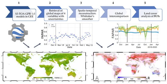
Figure 1.
Workflow for the generation of spatiotemporally reconstructed global maps of the four EVTs. The five main modules are presented with exemplary results.
2.2. S3-TOA-GPR-1.0 Models
A first prototype of the GPR-based hybrid EVT models was presented and validated by De Grave et al. [17,44]. The key steps performed to build the models started with simulating TOC reflectance for a multitude of leaf canopy states using the SCOPE model (v.1.7), for which the radiative transfer scheme is based on PROSPECT-D [45] and 4SAIL [46]. To generate TOC reflectance with SCOPE, leaf biochemical, canopy biophysical, soil, and geometry variables were defined with specified ranges and distributions. Additionally, a diversity of non-vegetated reflectance spectra were added to the training data to account for surface heterogeneity [17]. To successfully implement the models into GEE for global-scale processing of S3 data, however, the models needed to be adapted for running within the platform. Currently, GEE does not feature OLCI L2 reflectance data but provides the L1B product. Thus, the models had to be adapted to enable the processing of TOA radiance data. To achieve this, Reyes-Muñoz et al. [23] initially presented a workflow where the SCOPE TOC simulations were upscaled to TOA radiance data coupling with simulations coming from the atmospheric RTM 6SV (v.2.1) [24]. That workflow is here briefly described and further elaborated. A broad range of atmosphere and geometry scenarios were simulated to ensure that trained TOA models are generically applicable. The input variable values, ranges, and distributions for the SCOPE and 6SV models, as applied also in our study, are summarized in Table 1 and Table 2.

Table 1.
Biochemical leaf and canopy structure variables used for SCOPE simulations. See De Grave et al. [17] for details about default values.
Table 2.
6SV input variables used to simulate the atmospheric transfer functions.
An automated coupling process was realized with the Atmospheric Lookup table Generator (ALG) [47] and with the TOC2TOA toolbox from the Automated Radiative Transfer Models Operator (ARTMO) [48]. Similar to before, TOA radiance spectra of non-vegetated surfaces from different land covers and seasons were selected from S3 imagery (e.g., bare soils, rocks, and water bodies). This serves to provide robust training inputs and to obtain high-quality mapping performances over heterogeneous landscapes. It led to about 10% of non-vegetated spectra to the total training dataset per EVT.
GPR was chosen as the core retrieval algorithm [49,50]. GPR is a Bayesian supervised machine learning regression algorithm where predictor and target are continuous variables. The GPR method learns the relationship between the input samples and output observations. The similarity of samples and is quantified through a kernel function [51]. Among the multiple kernel functions available, the Asymmetric Square Exponential equation has been demonstrated to be efficient for vegetation modelling from EO data [52]. This function makes the assumption that the correlation between two input variables declines proportionally with their respective distance, signifying that closer points are expected to behave more similarly than the points placed further away from each other [53]. The process starts with using the observed and measured data and constraining the prior GP distribution to create a posterior GP function. The more data points, the lower the uncertainty, due to the function being better adjusted. The theory for uncertainty () has been experimentally demonstrated by Verrelst et al. [54]. For an exhaustive description of the S3-TOA-GPR-1.0 models and validation accuracy information of the generated maps, readers are referred to Reyes-Muñoz et al. [23].
2.3. S3-TOA-GPR-1.0 Model Implementation in Google Earth Engine
GEE is a powerful planetary-scale cloud-computing platform for Earth science data and analysis. GEE enables free programmatic access to global-scale Earth observation products. It has an interactive application programming interface (API) that allows users to quickly handle and visualize results with ease in the interactive development environment (IDE). Users can perform spatial calculations by having access to a multi-petabyte database and make requests through JavaScript or Python APIs that are sent by the client to Google via JSON objects [55]. Given the limitations of client–server data transfer, we followed the method by Pipia et al. [20] to implement the GPR models into GEE. In brief, it consists of expanding the standard GPR formulas through matrix algebra formulations, through the specific image-array datatype of GEE. The EVT products were retrieved by the GPR models in batches using the Python API, and consequently masked within GEE with bare land cover and water body masks. Additionally, according to the workflow presented by Reyes-Muñoz et al. [23], the OLCI L1B quality band [56] was used for classifying pixels as invalid, bright, or saturated, and these pixels were also excluded from the retrievals.
For uploading external files we used an open-source command line interface (CLI) by Samapriya [57] called geeup. Thus, global spatiotemporal products of the four EVTs were produced for the year 2019. For fast processing and memory-efficient exporting, the global GPR-derived products were mapped at a 5 km global resolution, for which each temporally composited map has a file size of 350–360 Megabytes. Note that for the nominal 300 m resolution, this increases up to 70 Gigabytes per global map.
2.4. Spatiotemporal Reconstruction with Whittaker Smoother Function
Since only the raw OLCI L1B product is provided in the GEE platform, cloud-flagging information is missing. To bypass this constraint, a solution was sought by filling cloud-induced gaps exclusively based on temporal patterns of the retrieved EVT data. Given that clouds typically emerge relatively short in time, signal reconstruction in the temporal domain through interpolation is commonly applied as a solution to fill cloud-induced gaps [58]. Among interpolation functions in time series analysis, the WS function is advantageous because it interpolates smoothly given the temporal observations, and at the same time provides control over the degree of smoothness with only one parameter: [35]. The function works in the following way. Suppose a noisy series y, which is predicted to have equal intervals and has a length of m. We aim to reach an accurate but smooth series z, to fit y without irregularities. However, the smoother the series z, the less accurately it shall fit the original y dataset [34]. The differences between two consecutive values of z can be expressed as:
By squaring and summing the differences, we obtain a clean and simple measure of roughness z:
Furthermore, if we sum the squares of the differences, we obtain S, which can be considered as the value that corresponds to the lack of fit of the data:
Thus, Q as the balanced sum of the two is calculated with , whose value is chosen by the user:
The goal of the penalized least squares method is to come up with a Q as low as possible. If a larger is chosen, that results in a stronger R influence on Q’s outcome, and z will be smoother. To aid calculations, matrices and vectors ought to be introduced:
where Each row contains the pattern −1 1, shifted such that and . D has m − 1 rows and m columns:
Equating the partial derivative of to zero, the linear system of equation is obtained:
where I is an identity matrix with m × m dimensions. It can be clearly seen in Equation (6) that the smoothed vector y depends on the penalty weight imposed by . Lower values of yield lower penalization, thus a rough curve, whereas when the weighing is increased, a smoother, but less accurate function is retrieved [59]. In order to select optimal values, the user has to visually assess the conformity of the smoothed series. This can be achieved by referring to the error values calculated between different series with different and assessing visually to select an adequate penalty weight value [34]. Finally, the GEE platform allows the implementation of the WS, so it is scalable to any time series data stream. The workflow for programming the WS presented by Khanal et al. [39] was taken as a basis and slightly modified to allow the function to run smoothly with S3-TOA-GPR-1.0 models in GEE. We chose to generate output maps at a 10-day temporall -composited resolution. The resulting reconstructed products are hereinafter referred to as S3-TOA-GPR-1.0-WS.
2.5. Reference Datasets
We cross-compared our estimates of the S3-TOA-GPR-1.0-WS models against established reference products. A correlation analysis was run per pixel on a global scale along the temporal domain. The selection criteria for reference products was the availability throughout the year 2019, to make intra-annual correlation possible.
For FAPAR and LAI, the reference products consisted of the MCD15A3H Version 6 MODIS Level 4 Terra and Aqua, corresponding to 4-day composite data sets in 500 m spatial resolution [60].
Our FVC product was compared against products from Copernicus Global Land Service (CGLS), originating from PROBA-V and SPOT [61]. This product is also smoothed and gap-filled. When the exact date of the retrieval differed from our maps, the products with the closest corresponding date were taken. The CGLS data sets were downloaded from https://land.copernicus.eu/global/themes/vegetation (accessed on 10 January 2023).
To our awareness, only a few global LCC products are publicly available and can suit our intercomparison analysis. For instance, no official LCC products have been produced by the MODIS or CGLS teams. Instead, we used the LCC product retrieved by Xu et al. [62] to verify the consistency of our LCC S3-TOA-GPR-1.0-WS models. This dataset is available on https://zenodo.org/record/5805575#.Y9ozrHZByUm (accessed on 10 January 2023). The product is a global 8-day LCC dataset at 500 m resolution which was generated between the years 2000 and 2020 from MODIS data using a multi-level matrix system with two pairs of vegetation indices. The locally adjusted cubic-spline capping (LACC) method was applied to fill gaps and smooth the LCC data set [62]. A summary of each reference dataset can be found in Table 3.
Table 3.
Reference datasets, EVT products, and their properties.
The MODIS MCD15A3H products, i.e., FAPAR and LAI, were already available on GEE. All the other reference datasets were first downloaded locally and subsequently resampled, reprojected, and then uploaded to GEE. The spatial resolution of the reference products was resampled to 5 km, and the nearest corresponding observation for our 10-day temporally composited retrievals was used for comparison. The LCC dataset’s nominal CRS was sinusoidal; thus, it had to be reprojected to the default WGS84 coordinate reference system (CRS). The CGLS (FAPAR, LAI, and FVC) and MOD09A1v006 (LCC) datasets were downloaded and uploaded to GEE in batches with geeup [57]. Regarding the usage of GEE, an aspect that could limit the uploading times for external data is the personal quota GEE assigns per user. The users are limited to a number of concurrently running up and downloading tasks (namely 3000) from the platform, and running numerous tasks in parallel could lead to longer uploading times [63].
2.6. Study Sites for Land Cover Analysis
To verify how different vegetated land covers affect the S3-TOA-GPR-1.0-WS retrieval method’s consistency, the 4 EVT products were correlated against corresponding MODIS and CGLS products. The effect of distinct types of land covers was investigated by superimposing specific land covers selected from the Copernicus Dynamic Land Cover (CGLS-LC100) database. The land covers were selected from the database as available within GEE [64]. Four study sites of approximately 400 × 400 km were selected. The locations of the study sites are indicated in Figure 2. Each region of interest (ROI) was carefully selected around the world in order to match the corresponding land cover. The criterion for selecting the locations of the ROIs was that the land cover of interest in each region must surpass 70% of the area of the region analyzed. The ROIs for the different land cover analyses were the following: (1) evergreen broadleaf rainforests over the Congo basin; (2) deciduous broadleaf forests over the Monongahela National Park in Western USA; (3) agricultural fields, consisting mainly of wheat and rice crops [65] over the Indo-Gangetic plains in India; and finally, (4) sparsely vegetated surfaces with very low vegetation cover and less pronounced yearly phenological dynamics over Western Australia. The exact location and percentage of land covers within the ROIs are represented in Table 4. Following this, land cover-specific comparisons against reference datasets were conducted calculating error metrics were calculated between our and reference products with representation of per-pixel p-values indicating statistical significance, and their corresponding temporal profiles were plotted within the ROIs using the land cover pixel’s averages.
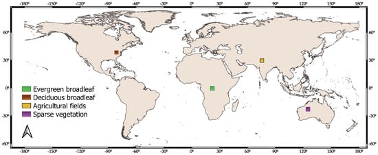
Figure 2.
Global distribution of the ROIs with the four different land covers.
Table 4.
Locations of the 500 × 500 km regions where land cover analysis was conducted. The percentage of the analyzed land cover’s area to the ROI’s area is also shown.
2.7. Statistical Evaluation
With the purpose of evaluating the spatiotemporal consistency of our S3-TOA-GPR-1.0-WS products, we correlated on a per-pixel basis all the data for the year 2019 to already existing and validated data sets explained in Section 2.6. For this intra-annual dataset, the Pearson correlation coefficient was then per-pixel calculated.
The Pearson correlation coefficient is a dimensionless index which is invariant to linear transformations of its variables. The values in the numerator are centered by subtracting out the mean of each variable, and the sum of cross-products for the center variable is calculated. The denominator is an adjustment for the variables to have equal units [66]. Equation (7) shows the mathematical formula to obtain R, the correlation coefficient:
Correlation coefficients indicate the strength of a linear relationship between two different variables x and y. When R is greater than zero, the relationship is positive, and when it is lower than zero, it is negative. A value of zero means no relationship between the variables exists [67]. Furthermore, root mean squared error (RMSE), normalized RMSE (NRMSE), as well the coefficient of determination (R) were calculated between S3-TOA-GPR-1.0-WS and the reference datasets. These calculations were run over the four selected ROIs. The equations of the error metrics are given below:
Consequently, by squaring R obtained from Equation (7), values were obtained. Finally, Pearson correlation and corresponding p-value maps showing statistical significance with additional statistical data were directly calculated and handled within the GEE platform. The p-value serves as an index measuring the strength of evidence against the null hypothesis that no significance exists on the given observations. p-values lower than 0.05 indicate evidence against the null hypothesis being tested [68].
3. Results
3.1. Global EVT Product Retrieval: Cloud-Gapped Maps
As expected, the first iteration of the global EVT products retrieved from the raw OLCI L1B TOA radiance data for the year 2019 produced gapped maps, mostly caused by cloud cover. The maps with zoomed-in regions where gaps were present are illustrated in Figure 3. These spatiotemporal gaps are the size of a few tens of pixels and exist for some daily observations. They are not visible when observing composited maps of mean pixel values for months or years. The gaps with a size of only a few pixels emerged for a shorter time span (1–2 observations) as opposed to the entire year’s temporal profile (∼36 observations). Most of these gaps have irregular sizes and were mainly caused by clouds and some by snow cover. The most apparent gaps were present along latitudes of 28° over Southeast Asia and 0° over the Amazon and the Congo Basin. Cloud cover also emerged over the British Isles and over latitudes of 50° by the Pacific coast of Canada and 70° in Russia. The resulting data discontinuity in both the spatial and temporal domains of the EVT products was resolved by creating new, temporally reconstructed maps, as addressed in Section 3.3.
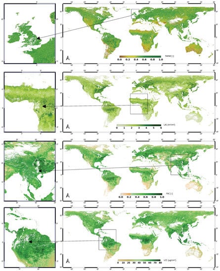
Figure 3.
Global EVT maps with gaps highlighted at specific regions before temporal reconstruction at 5 km resolution for 10 July 2019.
3.2. Uncertainty Maps
Apart from mean estimates of the targeted EVT, the Bayesian GPR algorithm also delivers associated uncertainty intervals. The maps displayed in Figure 4 present the spatial distribution of the S3-TOA-GPR-1.0 uncertainty, expressed as standard deviation (). Retrievals with high levels of uncertainty indicate pixels with spectral information that deviates from what was used during the training phase. Conversely, retrievals with low uncertainty refer to pixels that were well-represented in the training process. High uncertainties are caused by inaccuracies in the input data and model imperfections. They are estimated during the retrieval process and serve as a quality layer to filter out unreliable estimates. Areas with higher uncertainties include the southern border of the Sahara for mainly all the variables. For LCC and LAI, the Amazon region and generally northern latitudes indicate the highest uncertainties. However, when interpreting the uncertainty maps, it must be noted that values are related to the absolute values of the mean estimates. As an example, an LCC uncertainty value of = 4 g/cm would be critical for a mean LCC estimate of 4 g/cm. Conversely, = 4 g/cm can be considered as low uncertainty when the mean LCC is equal to 40 g/cm.
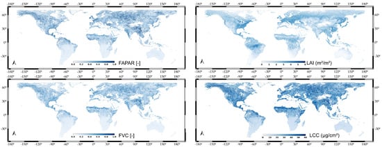
Figure 4.
Global uncertainty maps () of FAPAR, LAI, FVC, and LCC at 5 km resolution for 10 July 2019.
3.3. Whittaker Smoother and Spatiotemporally Reconstructed Cloud-Free Global Maps
Due to clouds, globally derived EVT maps are prone to gaps both in the spatial and temporal domains. To overcome these gaps, the WS interpolation technique was implemented. The performance of the WS was tuned by adjusting the value of the penalty weight , which controls the smoothness of the series. In order to find the optimal , several iterations were run for the year 2019 by changing , i.e., using values of 0.5, 1, 10, 100, 1000, and 10,000. The resulting R values between the series of S3-TOA-GPR-1.0-WS and the differently weighed WS series were then inspected. According to the error metrics and visual assessment, the most satisfactory fits of WS were obtained by using = 100. Five months were added at the beginning and end of the 2019 time window to achieve validly smoothed and reconstructed profiles for the entire annual time window. Such extension helps to avoid introducing unrealistic predictions at the tails (see also Figure 5). This practice is also applied by the TIMESAT software package, which has been extensively used in various research applications for the purpose of extracting phenology metrics, using the SG filter, which is similar in many of its aspects to WS function [30,69].
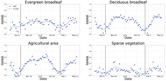
Figure 5.
Whittaker’s interpolating function applied to S3-TOA-GPR-1.0 retrievals of four different land covers with a of 100. The vertical lines indicate the start and end of the year 2019.
The WS function processed discrete values at the available daily pixel data and returned a continuous profile. The images were reprocessed throughout the entire data stream, thus yielding spatiotemporally continuous maps without gaps. The function was directly implemented into GEE; therefore, global temporally reconstructed maps can be managed within the platform. Figure 6 presents the resulting temporally reconstructed EVT maps for 10 July 2019 as generated by the S3-TOA-GPR-1.0-WS models at 5 km resolution. Although we demonstrate only results for 10 July 2019 (Figure 6), maps of any day of the year (2019) can be generated. A full, annual global data stream took only 20–30 s to reconstruct within GEE.
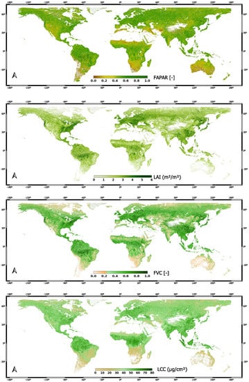
Figure 6.
Global EVT temporally reconstructed maps using the S3-TOA-GPR-1.0-WS models at 5 km spatial resolution, 10 July 2019.
3.4. Global Intra-Annual Correlation Maps against Reference Products
With the purpose of assessing the consistency of the global mapping, the Pearson correlation coefficient, R, was calculated between the S3-TOA-GPR-1.0-WS data stream and corresponding comparison datasets. In order to examine the temporal profiles for intercomparison, the year 2019 was extended with data ranging from August 2018 to May 2020. These extra months were not used to retrieve the global correlation maps (Figure 7 and Figure 8), where only data from 2019 were used. FAPAR and LAI were cross-compared against both MODIS and CGLS, FVC only against CGLS, and finally, LCC against MODIS for the year 2019. Globally averaged R values along with their standard deviation were also calculated. The general trend amongst all EVT correlation revealed that areas with pronounced vegetation dynamics correlated well with MODIS and CGLS products, whilst regions of low yearly change in vegetation yielded R values close to zero.
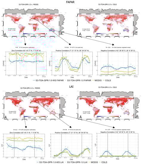
Figure 7.
Pearson correlation coefficients for FAPAR (top) and LAI (bottom) for the year 2019 between S3-TOA-GPR-1.0-WS models and datasets from MODIS and CGLS at 5 km spatial resolution. The global mean and standard deviation of the R correlation are also given. Examples of three distinct correlation values are highlighted with their corresponding temporal profiles. Both WS reconstructed (blue line) and original S3-TOA-GPR-1.0 values (light blue dots) are plotted. The vertical lines indicate the start and end of the year 2019.
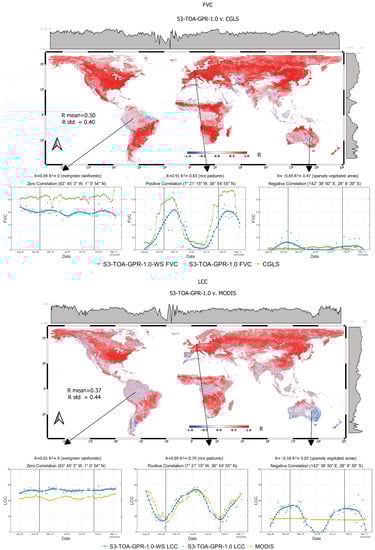
Figure 8.
Pearson correlation coefficients for FVC (top) and LCC (bottom) for the year 2019 between S3-TOA-GPR-1.0-WS models and MODIS CGLS dataset at 5 km spatial resolution. The global mean and standard deviation of the R correlation are also given. Examples of three distinct correlation values are highlighted with their corresponding temporal profiles. Both WS reconstructed (blue line) and original S3-TOA-GPR-1.0 values (light blue dots) are plotted. The vertical lines indicate the start and end of the year 2019.
The S3-TOA-GPR-1.0-WS models showed consistent results over latitudes with pronounced yearly vegetation phenology and agricultural croplands compared to the reference products. The models’ correlation consistency agreed closely over these land covers with 0.6. Lower correlation was found over sparsely vegetated areas where pronounced phenological dynamics are absent. When inspecting each EVT, we can conclude that the S3-TOA-GPR-1.0-WS models produce fairly consistent products across the globe. However, some discrepancies were found for FAPAR with an of 0.33 against both reference products and an of 0.38 for MODIS and 0.39 for CGLS. LAI proved to be the most consistent, with a mean global correlation of 0.52 against MODIS and the highest value against CGLS with standard deviations of similar magnitude as calculated for FAPAR. FVC produced similar error statistics as LAI, being the second most consistent variable on a global scale. It led to an of 0.50 and of 0.40. LCC, out of all EVTs, produced the highest , namely 0.44, while the correlation on a global scale was lower than the standard deviation, being = 0.37. For a quantitative comparison of the correlation maps, histograms are provided in Figure A1 and Pearson correlation-associated p-value maps are also presented in Figure A2. Additionally, Pearson correlation-associated p-value maps provide more information over the statistical significance of the R correlation maps. Areas with higher values include regions around the equator and sparsely vegetated areas over Australia and the Namibian desert. Areas that show no statistically significant correlations are mainly regions that have land covers such as evergreen broadleaf and sparse vegetation. Areas showing higher p-values mean that the observed correlation between the two time series is likely to have occurred by chance only. This can be observed on the temporal profiles in Figure 7 and Figure 8, showing two radically different temporal profiles for evergreen broadleaf and sparsely vegetated land covers. The null hypothesis, stating that no linear relationship exists between the two time series, cannot be rejected with such high p-values (greater than 0.05) [68].
Figure 7 and Figure 8 also present three specific cases where distinct correlation cases were present. Time series for high-, zero-, and low-correlation cases are shown, with gapped and temporally reconstructed EVT profiles. Furthermore, the latitudinal and longitudinal distributions of the R values are plotted along the maps.
The temporal profiles shown in Figure 7 and Figure 8 (left) depict cases where the correlation is around zero between S3-TOA-GPR-1.0-WS and reference products ( 0). The land covers with low yearly change in phenology tend towards these low correlations, which is also reflected in the latitudinal R distribution plot. For demonstration, we selected an exemplary site of the Amazon rainforest, where LAI, FAPAR, and FVC yearly profiles calculated from S3-TOA-GPR-1.0-WS models revealed underestimation compared to those of MODIS and CGLS products.
The temporal profiles shown in Figure 7 and Figure 8 (middle) demonstrate a high correlation ( 0.8) between the products, observed over agricultural areas on the Iberian Peninsula. Here, the S3-TOA-GPR-1.0-WS EVT model’s temporal profile is consistent with the comparison datasets’ for all EVTs. For LAI, the S3-TOA-GPR-1.0-WS model slightly overestimated both MODIS and CGLS estimates, whilst the FVC product tends to underestimate CGLS’s profile. The LCC temporal profile is in agreement with the MODIS LCC product. Accordingly, the latitudinal R distribution indicates a consistent R profile for all S3-TOA-GPR-1.0-WS products over the Northern Hemisphere.
Figure 7 and Figure 8 (right), demonstrates profiles with negatively correlated maps, which emerged especially over the Central Australian shrublands and are characterized by sparse herbaceous vegetation. Negative correlations between all four S3-TOA-GPR-1.0-WS EVT products and the reference products can be mainly found in deserts and regions with scarce vegetation cover.
Apparently, the S3-TOA-GPR-1.0-WS models produce stronger seasonal effects than MODIS and CGLS products, with values around LAI = 2 in the Australian summer, that are mostly caused by precipitation. The sparsely vegetated shrublands are sensitive to water and can reach LAI = 2 after few days of rain. These areas cause a drop in the R distribution profile that can be observed around −30° latitude, in the Southern Hemisphere.
3.5. Local Land Cover Analysis
Following the successful retrieval of the global EVT maps and the running of the WS temporal reconstruction function, the resulting annual cloud-free S3-TOA-GPR-1.0-WS data stream was correlated against corresponding MODIS and CGLS products over four distinct land covers within the ROIs (see Figure 2). These sites were selected due to their analyzed vegetated land cover being dominant over the area. The averaged temporal profiles over distinct vegetated land covers for the extended year 2019 can be observed in Figure 9. Goodness-of-fit statistics for each land cover can be found in Table 5. Surfaces marked by considerable phenological dynamics, particularly deciduous broadleaf forests and agricultural areas, obtained higher consistency. Cross-comparison for evergreen broadleaf forests and sparsely vegetated surfaces obtained a rather low R correlation, in the case of all four EVTs.
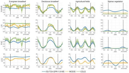
Figure 9.
Averaged temporal profiles with the shaded area as one standard deviation for selected vegetated land covers, as defined in Table 4. The vertical lines indicate the start and end of the year 2019.
Table 5.
Goodness-of-fit statistics of the S3-TOA-GPR-1.0-WS products vs. the reference products for selected vegetated land covers as defined in Table 4.
The closest agreements were obtained for the land covers with the greater annual variation in vegetation cover, namely deciduous broadleaf forests. For these land covers, R was always greater than 0.87 for each EVT, with the best-performing variable: FVC against CGLS with an R of 0.98 over deciduous broadleaf forests. The only zero-correlation case was produced by LCC against MODIS over the agricultural fields, where R was 0.26. For evergreen and deciduous broadleaf forests, LAI/FAPAR values of MODIS tend to reach higher maximum yearly values than those provided by the S3-TOA-GPR-1.0-WS models. The S3-TOA-GPR-1.0-WS FVC product consistently underestimates as opposed to the two other datasets. Also, the S3-TOA-GPR-1.0-WS underestimated LAI, FAPAR, and FVC for land covers with lower yearly changes in phenology, such as evergreen broadleaf forests, compared to MODIS and CGLS products. For shrublands or sparsely vegetated areas, S3-TOA-GPR-1.0-WS retrieved LAI ≈ 2 and FAPAR ≈ 0.4 during cold seasons (winter). The least consistency appeared for LCC against MODIS, where the best-performing land cover was deciduous broadleaf forests, with an R of 0.88; conversely, other vegetation land covers led to poorer correlations, with an R below 0.26.
4. Discussion
The integration of hybrid GPR models into GEE opened up new avenues in facilitating research activities in the field of vegetation trait mapping and monitoring. Although a few studies had examined the incorporation of GPR models into GEE for time series processing at regional to continental scale [20,21,23], the potential of the models for GEE-based time series processing at a global scale remained to be investigated. Therefore, we evaluated whether the hybrid EVT models can be likewise applied at the global scale, thereby preserving sufficient fidelity. In the following sections, we will discuss the results of the global processing of the four gap-free EVT products (Section 4.1), followed by the WS-based temporal reconstruction processing (Section 4.2) and intra-annual cross-comparison against reference FAPAR, LAI, FVC, and LCC products (Section 4.3). Finally, we will provide a critical discussion on limitations, challenges, and opportunities (Section 4.4 and Section 4.5).
4.1. Global Mapping of EVTs in GEE
GEE proved to be a versatile platform for fast retrieval of planetary-scale EVT maps and consequent temporal reconstruction. Its ability to process global datasets within a few seconds allows for the quick visualization of EVT products and for evaluating their consistency against reference data. Specifically being able to resample and reproject maps in a few seconds, GEE provides the option to compare products from different sensors [26,43]. To retrieve global EVT maps and cross-compare them intra-annually against reference datasets, the most important challenges to be tackled by GEE were the batch integration of external files and data such as CGLS products. In our experience, GEE is limited when handling large-scale operations with the involvement of external data.
Upon integration of the S3-TOA-GPR-1.0 models in GEE, as outlined in Section 2.3, it became feasible to process EVT maps on a global scale. Using the Python API to generate EVT maps in batches, the process did not take longer than 1 h for processing a full data stream of one year. The chosen temporal resolution of 10-day composites was adequate for analysis, as it balanced well between memory usage and output quality. Note that, for testing purposes, the global vegetation maps were exported in 500 m spatial resolution and had file sizes of roughly 70 Gigabytes of one EVT for a single 10 days temporal-composite observation. Our integrated workflow and the retrieval of S3-TOA-GPR-1.0-WS global EVT maps can be accessed and replicated by running the JavaScript code in GEE or the Python API in Google Colab and following the instructions on the GitHub page indicated in Appendix A.
4.2. Temporal Reconstruction Using the Whittaker Smoother
When expanding from regional towards global EO data processing, the requirement for resolving data discontinuities becomes more pressing. Throughout the retrieval process, the continuity of the data streams was mainly hindered due to cloud coverage. Aiming to replace those empty pixels with meaningful values, previous studies favored the usage of the WS function as a method for gap-free spatiotemporal reconstruction, e.g., [35,39,70,71]. One particular advantage of the WS is its superior performance against Fourier and Linear fit algorithms over stable land cover classes. This was also reported by Khanal et al. [39], who compared three temporal smoothers for distinct land covers. Furthermore, the WS possesses outstanding computational efficiency [72]; thus, its implementation in GEE is preferred as opposed to the weighted SGF, as also concluded by Zhang et al. [71]. Also in our study, the WS function succeeded in generating smooth, spatiotemporally continuous data streams.
Since the WS is a curve-fitting method, it requires sufficient data points in time to work adequately. Thus, the temporal reconstruction worked well in the case of smaller data gaps, as demonstrated in Figure 3. However, the reconstruction proved to be less accurate in the case of more extensive temporal gaps (the magnitude of several weeks). A decreasing consistency of the WS in case of larger data gaps was also reported by Kandasamy et al. [31].
To achieve optimally reconstructed gap-free time series here for the year 2019, the temporal domain used for calculating the WS had to be adjusted. If the WS was only fitted to the year 2019, the fitted curve’s consistency would decrease at the beginning and end of the year due to boundary effects. For this reason, the function was extended to ±5 months before and after 2019; see also Figure 5.
Distinct land covers have inherently different yearly temporal profiles; thus, it would be beneficial to obtain dynamically changing values for each. The study by Kong et al. [38] investigated varying and their performances over multiple land covers. The authors indicated that should be larger ( 10) in cloudy, equatorial regions with relatively high and constant vegetation cover. Over higher latitudes and regions with lower vegetation cover, must be smaller ( 5). Having examined a range of S3-TOA-GPR-1.0-WS profiles with varying and their statistical errors against non-smoothed S3-TOA-GPR-1.0 retrieval values, we chose the value of 100 due to its capability to be relatively accurate worldwide; it yields a smooth reconstructed curve without being affected by outliers. Amongst other curve-fitting algorithms, Kandasamy et al. [31] also analyzed the WS to fill gaps in MODIS LAI time series and confirmed that for the optimal results, should be 100. Note that decreasing did not notably enhance the overall accuracy (results not shown), but made the smoothed curve more susceptible to the influence of outliers within the data.
4.3. Intra-Annual Analysis of EVT Products over Distinct Land Covers
To evaluate the consistency of the S3-TOA-GPR-1.0-WS EVT products against the reference products, it was necessary to examine the models’ performances across different vegetation types. Each targeted vegetation cover (i.e., evergreen broadleaf and deciduous broadleaf forests, agricultural and sparsely vegetated areas) was selected from the Copernicus Dynamic Land Cover map database within the ROIs, while other regions were masked out.
There has been a slight underestimation of all four EVTs as opposed to the reference datasets over denser vegetated surfaces, such as evergreen forests. The anomalies encountered with our S3-TOA-GPR-1.0-WS LAI models could be explained by the differences in the algorithms employed to calculate an EVT value and the use of different LAI definitions for product estimates. For instance, the underestimation of S3-TOA-GPR-1.0-WS at high LAI values could result from the fact that our workflow assumes a turbid medium canopy that results in effective LAI, whilst the MODIS retrieval algorithm incorporates radiative transfer formulations taking into account vegetation clumping, thus yielding the total LAI. Similar shortcomings were also noted by Campos-Taberner et al. [43]. The authors also retrieved LAI maps using Landsat-7/8 and Sentinel-2A data using hybrid methods (i.e., RTM with random forests regression). By comparing their results to the MODIS LAI product, an analogous underestimation can be observed, especially over high LAI values arising from the fact that MODIS retrieval algorithm infers the total LAI.
Throughout the WS-based reconstruction of EVT time series, the S3-TOA-GPR-1.0-WS EVT temporal profiles showed less variability as compared to MODIS or CGLS, especially over evergreen broadleaf rainforests. Despite obtaining profiles that present fewer fluctuations throughout the investigated time domain, the smoothing effect could impose limitations, such as the under- and overestimation of EVT values. Since irregular EVT retrieval values were smoothed, it led to a lower amplitude of the temporal profile. Therefore, yearly minima and maxima values were not represented with such high consistency.
One possible reason for the inconsistencies between our and reference LCC products can be explained by the spectral data source used by the two methods for retrieval. In contrast to the S3-OLCI product, the MOD09A1v006 Terra surface reflectance product used by Xu et al. [62] does not include a red-edge band (≈680–750 nm). However, the spectral information of this specific region is highly relevant to obtain accurate LCC retrieval results [73]. Red-edge wavebands are covered by OLCI bands (bands O8 to O12) and used in our retrieval chain; thus, our models retrieve variables at a higher consistency.
Furthermore, some discrepancies were noticed over northern latitudes and the equator. These are mainly caused by long stretches of missing data due to persistent cloudiness or irregular EVT values resulting from residual clouds and snow contamination. Similar challenges were reported by Fuster et al. [61], who validated PROBA-V LAI, FAPAR, and FVC datasets. They also noted that there were greater differences between CGLS PROBA-V products for evergreen broadleaf forests in tropical areas and needle-leaf forests in northern latitudes.
4.4. Limitations and Challenges of Global EVT Mapping
Regarding the building of the S3-TOA-GPR-1.0-WS models, training data sets relied on benchmark vegetation and atmosphere RTMs, but they remain a simplification of reality. For instance, the turbid media assumptions of SCOPE, composed of PROSPECT-D [45] plus 4SAIL [46] models (=PROSAIL), may lead to limitations, but also provide multiple advantages. The SAIL model was predominantly validated on grassland and crop canopies that were homogeneous, rather than on heterogeneous forest stands, according to [74]. Yet, the coarse spatial resolution used in our study may compensate by integrating the detailed structure effect of heterogeneous stands. In general, studies confirmed that PROSAIL presents a good compromise between the realistic descriptions of the radiation regime within a canopy, model complexity, simulation accuracy, and computational requirements [75,76]. For further model improvements, additional training data can be introduced from forest 3D RTMs. However, at a coarse resolution in the order of hundreds of meters to kilometers, horizontal land cover heterogeneity plays a more important role in the radiation emission and scattering than in vertical distribution. The directional reflectances simulated by 1D and 3D models tend to converge at coarser spatial resolutions, typically beyond 100 m [77]. To account for surface heterogeneity, here, a diversity of non-vegetated spectra has been added to the training data, thereby respecting a trade-off to ensure that the models stay lightweight and easily implementable in GEE (up to 10% of total training datasets).
The limitations and inaccuracies resulting from different atmospheric factors when using TOA radiance must also be addressed. One specific challenge is correcting the strong impact of atmospheric gases including water vapor, carbon dioxide, ozone, and aerosols, as they can be highly variable in both space and time, and have complex scattering and absorbing properties that depend on factors such as size, shape, chemistry, and density [78]. These atmospheric gases can distort the consistency of remotely sensed data [79,80]. The aforementioned variability was addressed in our hybrid models by applying a random sub-sampling strategy from the pool of 6SV simulations. A few more limitations of the atmospheric 6SV RTM may play a minor role, such as the parallel plane assumption for the atmosphere [78].
Altogether, running the S3-TOA-GPR-1.0 models in combination with the WS function provides an effective framework for global cloud-free mapping of EVTs. Smaller data gaps were easily corrected by the temporal reconstruction of the WS. Both the S3-TOA-GPR-1.0 retrieval and the WS function encountered limitations imposed by the high cloud cover frequency between −15° and +15° latitudes when monitoring agricultural areas and evergreen rainforests. Optical data face limitations, especially throughout the September–February time span. To mitigate the EVT underestimation due to omnipresent cloud cover, fusion approaches together with complementary all-weather radar time series could be considered, e.g., as proposed by Pipia et al. [81] and applied by Caballero et al. [82].
In our experience, the WS function processed optimally at regular temporal profiles; however, when it encountered noisier temporal profiles, its performance decreased. For irregular temporal profiles, the asymmetric Gaussian method could give better predictions for the beginnings and ends of the seasons [83]. Despite the similarities between WS and the conventional SGF, the WS offers more advantages. One particular appealing advantage of WS is its higher speed and lower computational demands as opposed to SGF. Additionally, the WS provides continuous smoothness over the entire span of the series, whereas the SGF gives only a discrete control over the smoothness. Although both the WS and SGF encounter difficulties with irregular retrieval values, the WS is capable of interpolation of missing data of larger width, whereas the SGF can only work with smaller stretches of missing data that are covered by its working window. Even though WS faces limitations when interpolating larger stretches of missing data, its performance is still superior in this aspect to SGF [34]. Alternative approaches towards obtaining gap-free EVT maps are also possible. One particular approach executable within GEE is the HISTARFM algorithm, which uses a combination of multispectral imagery from various sensors to reduce noise and obtain monthly gap-free observations over land. The HISTARFM uses the bias-aware Bayesian algorithm data assimilation scheme with historical Landsat data and fused MODIS-Landsat data to retrieve interpolated surface reflectances. The main bottleneck of this approach is the high computational and memory burden. Unlike the WS, HISTARFM requires areas to be pre-processed and cannot be run quickly, in the order of seconds within GEE [26]. Altogether, the quoted advantages of WS and its seamless implementation in GEE provided a quick and robust way to obtain cloud-free global EVT maps.
4.5. Opportunities for Next-Version Model Optimization
The presented temporally reconstructed global cloud-free EVT products were only processed for the extended year 2019, yet the developed workflow can be easily applied to any available OLCI L1B date range from 24TH May 2016 onwards. The S3-TOA-GPR-1.0-WS global EVT models and codes are freely accessible, and local-to-global maps can be quickly generated on the GEE platform. This offers opportunities for the broader community to inspect and use the four EVT products in higher-level applications. For instance, such applications may include the assessment of multi-year trends and seasonal anomalies [21,25]. Global data streams of the EVT products can be used to further assimilate into models which estimate global gross primary productivity [84,85].
Thanks to the Bayesian nature of the GPR models, uncertainty intervals along with the mean estimates were provided. The uncertainty maps provide a way to evaluate the robustness of the GPR algorithm when trained by artificial spectra, e.g., generated by RTMs [54]. The measurement of uncertainties associated with EVTs is crucial when incorporating these products into higher-level processing operations [86]. To further improve our EVT products, introducing a quality threshold for unrealistically high values provides a way to flag or mask out highly uncertain retrieval pixel values. Although this option is not implemented here, such quality flags would be a convenient upgrade for the next iteration of the presented workflow.
The 5 km resolution for global mapping inevitably contained pixel heterogeneity. Further investigation using time series of in situ measurements is required for a better understanding of the causes of the observed disagreements between the different products [87]. The EVT models can be improved through additional training data at sites presenting negative correlations. Nonetheless, the GPR models can be run at the native 300 m resolution in GEE. One has to be careful with memory handling when aiming to process time series, but when restricting to dedicated regions, processing at 300 m is perfectly possible, e.g., over the Iberian Peninsula (see also Figure A3 for a direct visual comparison of the 300 m vs. 5 km resolution maps processed over the same area). For this region, the memory file size reached up to a gigabyte per temporally composited 300 m map.
Finally, in the framework of the S3-FLEX tandem mission concept, it is foreseen that the S3-TOA-GPR-1.0-WS models presented here will play a crucial role in the quantification of photosynthetic activity within assimilation processing chains once FLEX is operational and begins transmitting data [88,89].
5. Conclusions
We presented a scalable retrieval workflow for the global cloud-free production of four essential vegetation traits (FAPAR, LAI, FVC, LCC) based on S3 TOA radiance data. By implementing hybrid models (S3-TOA-GPR-1.0) into the GEE platform, we have successfully processed the four EVT products for the year 2019. Our workflow utilized a 5 km spatial resolution and observations at a temporal resolution of 10 days of the S3-OLCI TOA radiance (L1B) product. The novelty of the GPR algorithm is the model’s associated per-pixel uncertainties, which can be used to assess the fidelity of the predictions. For instance, the uncertainty information serves to identify spectral surfaces that are less well-presented by the training data sets. Due to the absence of cloud screening in the L1B radiance product, we applied reconstruction of the data stream across the temporal domain using the Whittaker smoother function. The WS function processed the global EVT data streams almost instantaneously in GEE, resulting in cloud-free, spatiotemporally continuous maps (S3-TOA-GPR-1.0-WS). Global cross-comparison of the S3-TOA-GPR-1.0-WS products against reference products suggested a moderate-to-high correlation depending on the EVT, vegetation type, and geographic location. On a global scale, the generated EVTs behaved consistently along 30–60° latitude over the Northern Hemisphere. The most consistently mapped EVT was LAI, which yielded a globally averaged correlation of R = 0.57. The specific land cover analysis over local 400 × 400 km sites showed FVC to respond in closest agreement with the corresponding CGLS product over deciduous broadleaf forests in the Monongahela National Park in Western USA (R of 0.98). For all EVTs, the S3-TOA-GPR-1.0-WS produced generally consistent values over regions marked by pronounced yearly phenological dynamics, which led to strong correlations against reference products.
Ultimately, the presented processing scheme is anticipated to support the interpretation of terrestrial SIF observations delivered by the upcoming FLEX mission that will orbit in tandem with S3, thus enabling global monitoring of vegetation’s health and productivity dynamics at 300 m pixel resolution.
Author Contributions
D.D.K.—Conceptualization, Methodology, Software, Writing—original draft. P.R.-M.—Conceptualization, Methodology, Resources, Writing—Review and Editing. M.S.-D.—Resources, Writing—Review and Editing. V.I.M.—Software, Data Curation, Visualization. K.B.—Conceptualization, Methodology, Formal analysis, Writing—original draft. J.V.—Conceptualization, Methodology, Formal analysis, Writing—original draft. All authors have read and agreed to the published version of the manuscript.
Funding
The research was funded by the European Research Council (ERC) under the ERC-2017-STG SENTIFLEX project. Grant number: 755617. The ESA’s Land surface Carbon Constellation (LCC) project (4000131497/20/NL/CT) also partially supported this research.
Data Availability Statement
The code for the processing of the global cloud-free EVT maps can be accessed via https://github.com/daviddkovacs/Global-EVT-maps (accessed on 1 July 2023).
Conflicts of Interest
The authors declare no conflict of interest.
Appendix A

Figure A1.
Histograms with descriptive statistics showing the frequency of the R values as calculated over the 2019 window for the GPR models against reference products over the world.
Figure A1.
Histograms with descriptive statistics showing the frequency of the R values as calculated over the 2019 window for the GPR models against reference products over the world.


Figure A2.
Pearson correlation-associated global distribution of p-values at 5 km spatial resolution. Regions with p-values < 0.05 are considered to be statistically significant.
Figure A2.
Pearson correlation-associated global distribution of p-values at 5 km spatial resolution. Regions with p-values < 0.05 are considered to be statistically significant.


Figure A3.
EVT maps over the Iberian Peninsula at 300 m and 5 km resolution, 10 July 2019.
Figure A3.
EVT maps over the Iberian Peninsula at 300 m and 5 km resolution, 10 July 2019.


References
- ESA. ESA’s Living Planet Programme: Scientific Achievements and Future Challenges. Scientific Context of the Earth Observation Science Strategy for ESA; European Space Agency: Noordwijk, The Netherlands, 2015. [Google Scholar]
- Moreno, J.; Goulas, Y.; Huth, A.; Middleton, E.; Miglietta, F.; Mohammed, G.; Nedbal, L.; Rascher, U.; Verhoef, W.; Drusch, M.; et al. Report for mission selection: FLEX. ESA SP 2015, 1330, 3. [Google Scholar]
- Pinty, B.; Lavergne, T.; Widlowski, J.L.; Gobron, N.; Verstraete, M.M. On the need to observe vegetation canopies in the near-infrared to estimate visible light absorption. Remote Sens. Environ. 2009, 113, 10–23. [Google Scholar] [CrossRef]
- Knorr, W.; Kaminski, T.; Scholze, M.; Gobron, N.; Pinty, B.; Giering, R.; Mathieu, P.P. Carbon cycle data assimilation with a generic phenology model. J. Geophys. Res. Biogeosci. 2010, 115. [Google Scholar] [CrossRef]
- Weiss, M.; Frederic, B.; Smith, G.; Jonckheere, I.; Coppin, P. Review of methods for in situ leaf area index (LAI) determination: Part II. Estimation of LAI, errors and sampling. Agric. For. Meteorol. 2004, 121, 37–53. [Google Scholar] [CrossRef]
- Kaminski, T.; Knorr, W.; Scholze, M.; Gobron, N.; Pinty, B.; Giering, R.; Mathieu, P.P. Consistent assimilation of MERIS FAPAR and atmospheric CO2 into a terrestrial vegetation model and interactive mission benefit analysis. Biogeosciences 2012, 9, 3173–3184. [Google Scholar] [CrossRef]
- Chen, J.M.; Black, T.A. Defining leaf area index for non-flat leaves. Plant Cell Environ. 1992, 15, 421–429. [Google Scholar] [CrossRef]
- Bréda, N.J.J. Ground-based measurements of leaf area index: A review of methods, instruments and current controversies. J. Exp. Bot. 2003, 54, 2403–2417. [Google Scholar] [CrossRef]
- Liang, S.; Wang, J. Fractional vegetation cover. In Advanced Remote Sensing, 2nd ed.; Academic Press: Cambridge, MA, USA, 2020; pp. 477–510. [Google Scholar]
- Zeng, X.; Dickinson, R.E.; Walker, A.; Shaikh, M.; DeFries, R.S.; Qi, J. Derivation and Evaluation of Global 1-km Fractional Vegetation Cover Data for Land Modeling. J. Appl. Meteorol. Climatol. 2000, 39, 826–839. [Google Scholar] [CrossRef]
- Curran, P.J.; Dungan, J.L.; Gholz, H.L. Exploring the relationship between reflectance red edge and chlorophyll content in slash pine. Tree Physiol. 1990, 7, 33–48. [Google Scholar] [CrossRef]
- Gitelson, A.A.; Gritz, Y.; Merzlyak, M.N. Relationships between leaf chlorophyll content and spectral reflectance and algorithms for non-destructive chlorophyll assessment in higher plant leaves. J. Plant Physiol. 2003, 160, 271–282. [Google Scholar] [CrossRef]
- Albero Peralta, E.; Lopez-Baeza, E.; Lidon Cerezuela, A.; Bautista Carrascosa, I.; Lull Noguera, C. Validation of OGVI (OLCI Global Vegetation Index) and OTCI (OLCI Terrestrial Chlorophyll Index) provided by the OLCI (Ocean and Land Color Instrument) sensor at the Valencia Anchor Station. 42nd COSPAR Sci. Assem. 2018, 42, 1–2. [Google Scholar]
- Gobron, N.; Morgan, O.; Adams, J.; Brown, L.A.; Cappucci, F.; Dash, J.; Lanconelli, C.; Marioni, M.; Robustelli, M. Evaluation of Sentinel-3A and Sentinel-3B ocean land colour instrument green instantaneous fraction of absorbed photosynthetically active radiation. Remote Sens. Environ. 2022, 270, 112850. [Google Scholar] [CrossRef]
- Donlon, C.; Berruti, B.; Buongiorno, A.; Ferreira, M.H.; Féménias, P.; Frerick, J.; Goryl, P.; Klein, U.; Laur, H.; Mavrocordatos, C.; et al. The Global Monitoring for Environment and Security (GMES) Sentinel-3 mission. Remote Sens. Environ. 2012, 120, 37–57. [Google Scholar] [CrossRef]
- Bourg, L.; Bruniquel, J.; Morris, H.; Dash, J. Copernicus Sentinel-3 OLCI Land User Handbook. 2021. Available online: https://sentinel.esa.int/documents/247904/4598066/Sentinel-3-OLCI-Land-Handbook.pdf (accessed on 1 July 2023).
- De Grave, C.; Verrelst, J.; Morcillo-Pallarés, P.; Pipia, L.; Rivera-Caicedo, J.P.; Amin, E.; Belda, S.; Moreno, J. Quantifying vegetation biophysical variables from the Sentinel-3/FLEX tandem mission: Evaluation of the synergy of OLCI and FLORIS data sources. Remote Sens. Environ. 2020, 251, 112101. [Google Scholar] [CrossRef]
- Verrelst, J.; Malenovský, Z.; der Tol, C.V.; Camps-Valls, G.; Gastellu-Etchegorry, J.P.; Lewis, P.; North, P.; Moreno, J. Quantifying Vegetation Biophysical Variables from Imaging Spectroscopy Data: A Review on Retrieval Methods. Surv. Geophys. 2019, 40, 589–629. [Google Scholar] [CrossRef]
- Van Der Tol, C.; Verhoef, W.; Timmermans, J.; Verhoef, A.; Su, Z. An integrated model of soil-canopy spectral radiances, photosynthesis, fluorescence, temperature and energy balance. Biogeosciences 2009, 6, 3109–3129. [Google Scholar] [CrossRef]
- Pipia, L.; Amin, E.; Belda, S.; Salinero-Delgado, M.; Verrelst, J. Green LAI Mapping and Cloud Gap-Filling Using Gaussian Process Regression in Google Earth Engine. Remote Sens. 2021, 13, 403. [Google Scholar] [CrossRef]
- Salinero-Delgado, M.; Estévez, J.; Pipia, L.; Belda, S.; Berger, K.; Paredes Gómez, V.; Verrelst, J. Monitoring Cropland Phenology on Google Earth Engine Using Gaussian Process Regression. Remote Sens. 2021, 14, 146. [Google Scholar] [CrossRef]
- Estévez, J.; Salinero-Delgado, M.; Berger, K.; Pipia, L.; Rivera-Caicedo, J.P.; Wocher, M.; Reyes-Muñoz, P.; Tagliabue, G.; Boschetti, M.; Verrelst, J. Gaussian processes retrieval of crop traits in Google Earth Engine based on Sentinel-2 top-of-atmosphere data. Remote Sens. Environ. 2022, 273, 112958. [Google Scholar] [CrossRef]
- Reyes-Muñoz, P.; Pipia, L.; Salinero-Delgado, M.; Belda, S.; Berger, K.; Estévez, J.; Morata, M.; Rivera-Caicedo, J.P.; Verrelst, J. Quantifying Fundamental Vegetation Traits over Europe Using the Sentinel-3 OLCI Catalogue in Google Earth Engine. Remote Sens. 2022, 14, 1347. [Google Scholar] [CrossRef]
- Vermote, E.; Tanré, D.; Deuzé, J.; Herman, M.; Morcrette, J.J. Second simulation of the satellite signal in the solar spectrum, 6S: An overview. IEEE Trans. Geosci. Remote Sens. 1997, 35, 675–686. [Google Scholar] [CrossRef]
- Atkinson, P.M.; Jeganathan, C.; Dash, J.; Atzberger, C. Inter-comparison of four models for smoothing satellite sensor time-series data to estimate vegetation phenology. Remote Sens. Environ. 2012, 123, 400–417. [Google Scholar] [CrossRef]
- Moreno-Martínez, Á.; Izquierdo-Verdiguier, E.; Maneta, M.P.; Camps-Valls, G.; Robinson, N.; Muñoz-Marí, J.; Sedano, F.; Clinton, N.; Running, S.W. Multispectral high resolution sensor fusion for smoothing and gap-filling in the cloud. Remote Sens. Environ. 2020, 247, 111901. [Google Scholar] [CrossRef] [PubMed]
- Huete, A.; Didan, K.; Miura, T.; Rodriguez, E.P.; Gao, X.; Ferreira, L.G. Overview of the radiometric and biophysical performance of the MODIS vegetation indices. Remote Sens. Environ. 2002, 83, 195–213. [Google Scholar] [CrossRef]
- Brinckmann, S.; Trentmann, J.; Ahrens, B. Homogeneity Analysis of the CM SAF Surface Solar Irradiance Dataset Derived from Geostationary Satellite Observations. Remote Sens. 2013, 6, 352–378. [Google Scholar] [CrossRef]
- Roy, D.P.; Ju, J.; Lewis, P.; Schaaf, C.; Gao, F.; Hansen, M.; Lindquist, E. Multi-temporal MODIS–Landsat data fusion for relative radiometric normalization, gap filling, and prediction of Landsat data. Remote Sens. Environ. 2008, 112, 3112–3130. [Google Scholar] [CrossRef]
- Zeng, L.; Wardlow, B.D.; Xiang, D.; Hu, S.; Li, D. A review of vegetation phenological metrics extraction using time-series, multispectral satellite data. Remote Sens. Environ. 2020, 237, 111511. [Google Scholar] [CrossRef]
- Kandasamy, S.; Baret, F.; Verger, A.; Neveux, P.; Weiss, M. A comparison of methods for smoothing and gap filling time series of remote sensing observations – application to MODIS LAI products. Biogeosciences 2013, 10, 4055–4071. [Google Scholar] [CrossRef]
- Beck, P.S.; Atzberger, C.; Høgda, K.A.; Johansen, B.; Skidmore, A.K. Improved monitoring of vegetation dynamics at very high latitudes: A new method using MODIS NDVI. Remote Sens. Environ. 2006, 100, 321–334. [Google Scholar] [CrossRef]
- Whittaker, E.T. On a New Method of Graduation. Proc. Edinb. Math. Soc. 1922, 41, 63–75. [Google Scholar] [CrossRef]
- Eilers, P.H.C. A Perfect Smoother. Anal. Chem. 2003, 75, 3631–3636. [Google Scholar] [CrossRef]
- Atzberger, C.; Eilers, P.H.C. International Journal of Digital Earth A time series for monitoring vegetation activity and phenology at 10-daily time steps covering large parts of South America. Int. J. Digit. Earth 2011, 4, 365–386. [Google Scholar] [CrossRef]
- Geng, L.; Ma, M.; Wang, X.; Yu, W.; Jia, S.; Wang, H. Comparison of Eight Techniques for Reconstructing Multi-Satellite Sensor Time-Series NDVI Data Sets in the Heihe River Basin, China. Remote Sens. 2014, 6, 2024–2049. [Google Scholar] [CrossRef]
- Shao, Y.; Lunetta, R.S.; Wheeler, B.; Iiames, J.S.; Campbell, J.B. An evaluation of time-series smoothing algorithms for land-cover classifications using MODIS-NDVI multi-temporal data. Remote Sens. Environ. 2016, 174, 258–265. [Google Scholar] [CrossRef]
- Kong, D.; Zhang, Y.; Gu, X.; Wang, D. A robust method for reconstructing global MODIS EVI time series on the Google Earth Engine. ISPRS J. Photogramm. Remote Sens. 2019, 155, 13–24. [Google Scholar] [CrossRef]
- Khanal, N.; Matin, M.A.; Uddin, K.; Poortinga, A.; Chishtie, F.; Tenneson, K.; Saah, D. A comparison of three temporal smoothing algorithms to improve land cover classification: A case study from Nepal. Remote Sens. 2020, 12, 2888. [Google Scholar] [CrossRef]
- Xie, F.; Fan, H. Deriving drought indices from MODIS vegetation indices (NDVI/EVI) and Land Surface Temperature (LST): Is data reconstruction necessary? Int. J. Appl. Earth Obs. Geoinf. 2021, 101, 102352. [Google Scholar] [CrossRef]
- Yang, X.; Meng, F.; Fu, P.; Wang, Y.; Liu, Y. Time-frequency optimization of RSEI: A case study of Yangtze River Basin. Ecol. Indic. 2022, 141, 109080. [Google Scholar] [CrossRef]
- Martínez-Ferrer, L.; Moreno-Martínez, Á.; Campos-Taberner, M.; García-Haro, F.J.; Muñoz-Marí, J.; Running, S.W.; Kimball, J.; Clinton, N.; Camps-Valls, G. Quantifying uncertainty in high resolution biophysical variable retrieval with machine learning. Remote Sens. Environ. 2022, 280, 113199. [Google Scholar] [CrossRef]
- Campos-Taberner, M.; Moreno-Martínez, Á.; García-Haro, F.J.; Camps-Valls, G.; Robinson, N.P.; Kattge, J.; Running, S.W. Global Estimation of Biophysical Variables from Google Earth Engine Platform. Remote Sens. 2018, 10, 1167. [Google Scholar] [CrossRef]
- De Grave, C.; Pipia, L.; Siegmann, B.; Morcillo-Pallarés, P.; Rivera-Caicedo, J.P.; Moreno, J.; Verrelst, J. Retrieving and validating leaf and canopy chlorophyll content at moderate resolution: A multiscale analysis with the sentinel-3 OLCI sensor. Remote Sens. 2021, 13, 1419. [Google Scholar] [CrossRef] [PubMed]
- Féret, J.B.; Gitelson, A.A.; Noble, S.D.; Jacquemoud, S. PROSPECT-D: Towards modeling leaf optical properties through a complete lifecycle. Remote Sens. Environ. 2017, 193, 204–215. [Google Scholar] [CrossRef]
- Verhoef, W.; Jia, L.; Xiao, Q.; Su, Z. Unified Optical-Thermal Four-Stream Radiative Transfer Theory for Homogeneous Vegetation Canopies. IEEE Trans. Geosci. Remote Sens. 2007, 45, 1808–1822. [Google Scholar] [CrossRef]
- Vicent, J.; Verrelst, J.; Sabater, N.; Alonso, L.; Rivera-Caicedo, J.P.; Martino, L.; Muñoz Marí, J.; Moreno, J. Comparative analysis of atmospheric radiative transfer models using the Atmospheric Look-up table Generator (ALG) toolbox (version 2.0). Geosci. Model Dev. 2020, 13, 1945–1957. [Google Scholar] [CrossRef]
- Verrelst, J.; Romijn, E.; Kooistra, L. Mapping Vegetation Density in a Heterogeneous River Floodplain Ecosystem Using Pointable CHRIS/PROBA Data. Remote Sens. 2012, 4, 2866–2889. [Google Scholar] [CrossRef]
- Verrelst, J.; Alonso, L.; Camps-Valls, G.; Delegido, J.; Moreno, J. Retrieval of vegetation biophysical parameters using Gaussian process techniques. IEEE Trans. Geosci. Remote Sens. 2012, 50, 1832–1843. [Google Scholar] [CrossRef]
- Verrelst, J.; Muñoz, J.; Alonso, L.; Delegido, J.; Rivera, J.P.; Camps-Valls, G.; Moreno, J. Machine learning regression algorithms for biophysical parameter retrieval: Opportunities for Sentinel-2 and-3. Remote Sens. Environ. 2012, 118, 127–139. [Google Scholar] [CrossRef]
- Rasmussen, C.; Williams, C. Gaussian Processes for Machine Learning; The MIT Press: Cambridge, MA, USA, 2006. [Google Scholar]
- Camps-Valls, G.; Verrelst, J.; Munoz-Mari, J.; Laparra, V.; Mateo-Jimenez, F.; Gomez-Dans, J. A Survey on Gaussian Processes for Earth-Observation Data Analysis: A Comprehensive Investigation; A Survey on Gaussian Processes for Earth-Observation Data Analysis: A Comprehensive Investigation. IEEE Geosci. Remote Sens. Mag. 2016, 4, 58–78. [Google Scholar] [CrossRef]
- Schulz, E.; Speekenbrink, M.; Krause, A. A tutorial on Gaussian process regression: Modelling, exploring, and exploiting functions. J. Math. Psychol. 2018, 85, 1–16. [Google Scholar] [CrossRef]
- Verrelst, J.; Rivera, J.P.; Moreno, J.; Camps-Valls, G. Gaussian processes uncertainty estimates in experimental Sentinel-2 LAI and leaf chlorophyll content retrieval. ISPRS J. Photogramm. Remote Sens. 2013, 86, 157–167. [Google Scholar] [CrossRef]
- Gorelick, N.; Hancher, M.; Dixon, M.; Ilyushchenko, S.; Thau, D.; Moore, R. Google Earth Engine: Planetary-scale geospatial analysis for everyone. Remote Sens. Environ. 2017, 202, 18–27. [Google Scholar] [CrossRef]
- ESA. Sentinel-3 OLCI Technical Guide. Available online: https://sentinels.copernicus.eu/web/sentinel/technical-guides/sentinel-3-olci (accessed on 28 February 2023).
- Samapriya, R. Samapriya/Geeup: Geeup: Simple CLI for Earth Engine Uploads (0.6.2). 2023. Available online: https://samapriya.github.io/geeup/ (accessed on 10 January 2023).
- Pipia, L.; Belda, S.; Franch, B.; Verrelst, J. Trends in Satellite Sensors and Image Time Series Processing Methods for Crop Phenology Monitoring. 2022. Available online: https://link.springer.com/chapter/10.1007/978-3-030-84144-7_8 (accessed on 13 July 2022).
- Zuliana, S.U.; Perperoglou, A. Two dimensional smoothing via an optimised Whittaker smoother. Big Data Anal. 2017, 2, 6. [Google Scholar] [CrossRef]
- Myneni, R.; Knyazikhin, Y.; Park, T. MCD15A3H MODIS/Terra+Aqua Leaf Area Index/FPAR 4-day L4 Global 500 m SIN Grid V006. 2015. Available online: https://ladsweb.modaps.eosdis.nasa.gov/missions-and-measurements/products/MCD15A3H (accessed on 1 July 2023).
- Fuster, B.; Sánchez-Zapero, J.; Camacho, F.; García-Santos, V.; Verger, A.; Lacaze, R.; Weiss, M.; Baret, F.; Smets, B. Quality Assessment of PROBA-V LAI, fAPAR and fCOVER Collection 300 m Products of Copernicus Global Land Service. Remote Sens. 2020, 12, 1017. [Google Scholar] [CrossRef]
- Xu, M.; Liu, R.; Chen, J.M.; Liu, Y.; Wolanin, A.; Croft, H.; He, L.; Shang, R.; Ju, W.; Zhang, Y.; et al. A 21-Year Time Series of Global Leaf Chlorophyll Content Maps From MODIS Imagery. IEEE Trans. Geosci. Remote Sens. 2022, 60, 1–13. [Google Scholar] [CrossRef]
- Google. Processing Environments | Google Earth Engine | Google Developers. 2022. Available online: https://earthengine.google.com/ (accessed on 23 February 2022).
- Buchhorn, M.; Bertels, L.; Smets, B.; Roo, B.D.; Lesiv, M.; Tsendbazar, N.E.; Masiliunas, D.; Li, L. Copernicus Global Land Service: Land Cover 100m: Version 3 Globe 2015–2019: Algorithm Theoretical Basis Document. Zenodo 2021. [Google Scholar] [CrossRef]
- Panigrahy, S.; Upadhyay, G.; Ray, S.; Parihar, J. Mapping of cropping system for the Indo-Gangetic plain using multi-date SPOT NDVI-VGT data. J. Indian Soc. Remote Sens. 2010, 38, 627–632. [Google Scholar] [CrossRef]
- Rodgers, J.L.; Nicewander, W.A. Thirteen Ways to Look at the Correlation Coefficient. Am. Stat. 1988, 42, 59–66. [Google Scholar] [CrossRef]
- Nickolas, S.; Mansa, J.; Katrina, M. Correlation Coefficients: Positive, Negative, & Zero. 2021. Available online: https://www.investopedia.com/ask/answers/032515/what-does-it-mean-if-correlation-coefficient-positive-negative-or-zero.asp (accessed on 1 July 2023).
- Chakkera, H.; Schold, J.; Kaplan, B. P Value: Significance Is Not All Black and White. Transplantation 2016, 100, 1607–1609. [Google Scholar] [CrossRef]
- Eklundh, L.; Jönsson, P. TIMESAT: A Software Package for Time-Series Processing and Assessment of Vegetation Dynamics. In Remote Sensing Time Series: Revealing Land Surface Dynamics; Kuenzer, C., Dech, S., Wagner, W., Eds.; Springer International Publishing: Cham, Switzerland, 2015; pp. 141–158. [Google Scholar] [CrossRef]
- Klisch, A.; Atzberger, C. Operational Drought Monitoring in Kenya Using MODIS NDVI Time Series. Remote Sens. 2016, 8, 267. [Google Scholar] [CrossRef]
- Zhang, Y.; Kong, D.; Gan, R.; Chiew, F.H.S.; McVicar, T.R.; Zhang, Q.; Yang, Y. Coupled estimation of 500 m and 8-day resolution global evapotranspiration and gross primary production in 2002–2017. Remote Sens. Environ. 2019, 222, 165–182. [Google Scholar] [CrossRef]
- Caballero, G.; Pezzola, A.; Winschel, C.; Casella, A.; Sanchez Angonova, P.; Orden, L.; Berger, K.; Verrelst, J.; Delegido, J. Quantifying Irrigated Winter Wheat LAI in Argentina Using Multiple Sentinel-1 Incidence Angles. Remote Sens. 2022, 14, 5867. [Google Scholar] [CrossRef]
- Xie, Q.; Dash, J.; Huang, W.; Peng, D.; Qin, Q.; Mortimer, H.; Casa, R.; Pignatti, S.; Laneve, G.; Pascucci, S.; et al. Vegetation Indices Combining the Red and Red-Edge Spectral Information for Leaf Area Index Retrieval. IEEE J. Sel. Top. Appl. Earth Obs. Remote Sens. 2018, 11, 1482–1493. [Google Scholar] [CrossRef]
- Jacquemoud, S.; Verhoef, W.; Baret, F.; Bacour, C.; Zarco-Tejada, P.J.; Asner, G.P.; François, C.; Ustin, S.L. PROSPECT+SAIL models: A review of use for vegetation characterization. Remote Sens. Environ. 2009, 113, S56–S66. [Google Scholar] [CrossRef]
- Cernicharo, J.; Verger, A.; Camacho, F. Empirical and Physical Estimation of Canopy Water Content from CHRIS/PROBA Data. Remote Sens. 2013, 5, 5265–5284. [Google Scholar] [CrossRef]
- Berger, K.; Atzberger, C.; Danner, M.; D’Urso, G.; Mauser, W.; Vuolo, F.; Hank, T. Evaluation of the PROSAIL Model Capabilities for Future Hyperspectral Model Environments: A Review Study. Remote Sens. 2018, 10, 85. [Google Scholar] [CrossRef]
- Widlowski, J.L.; Pinty, B.; Lavergne, T.; Verstraete, M.M.; Gobron, N. Using 1-D models to interpret the reflectance anisotropy of 3-D canopy targets: Issues and caveats. IEEE Trans. Geosci. Remote Sens. 2005, 43, 2008–2017. [Google Scholar] [CrossRef]
- Vermote, E.; Justice, C.; Claverie, M.; Franch, B. Preliminary analysis of the performance of the Landsat 8/OLI land surface reflectance product. Remote Sens. Environ. 2016, 185, 46–56. [Google Scholar] [CrossRef]
- Kaufman, Y.; Gao, B.C. Remote sensing of water vapor in the near IR from EOS/MODIS. IEEE Trans. Geosci. Remote Sens. 1992, 30, 871–884. [Google Scholar] [CrossRef]
- Li, Z.L.; Tang, B.H.; Wu, H.; Ren, H.; Yan, G.; Wan, Z.; Trigo, I.F.; Sobrino, J.A. Satellite-derived land surface temperature: Current status and perspectives. Remote Sens. Environ. 2013, 131, 14–37. [Google Scholar] [CrossRef]
- Pipia, L.; Muñoz-Marí, J.; Amin, E.; Belda, S.; Camps-Valls, G.; Verrelst, J. Fusing optical and SAR time series for LAI gap filling with multioutput Gaussian processes. Remote Sens. Environ. 2019, 235, 111452. [Google Scholar] [CrossRef]
- Caballero, G.; Pezzola, A.; Winschel, C.; Sanchez Angonova, P.; Casella, A.; Orden, L.; Salinero-Delgado, M.; Reyes-Muñoz, P.; Berger, K.; Delegido, J.; et al. Synergy of Sentinel-1 and Sentinel-2 Time Series for Cloud-Free Vegetation Water Content Mapping with Multi-Output Gaussian Processes. Remote Sens. 2023, 15, 1822. [Google Scholar] [CrossRef]
- Jönsson, J.; Eklundh, L. TIMESAT—A program for analysing time-series of satellite sensor data. Comput. Geosci. 2004, 30, 833–845. [Google Scholar] [CrossRef]
- Kaminski, T.; Knorr, W.; Scholze, M.; Gobron, N.; Pinty, B.; Giering, R.; Mathieu, P. Simultaneous Assimilation of FAPAR and Atmospheric CO2 into a Terrestrial Vegetation Model. In EGU General Assembly Conference Abstracts; NASA: Washington, DC, USA, 2012; p. 11748. [Google Scholar]
- Kaminski, T.; Knorr, W.; Schürmann, G.; Scholze, M.; Rayner, P.J.; Zaehle, S.; Blessing, S.; Dorigo, W.; Gayler, V.; Giering, R.; et al. The BETHY/JSBACH Carbon Cycle Data Assimilation System: Experiences and challenges. J. Geophys. Res. Biogeosci. 2013, 118, 1414–1426. [Google Scholar] [CrossRef]
- Jägermeyr, J.; Gerten, D.; Lucht, W.; Hostert, P.; Migliavacca, M.; Nemani, R. A high-resolution approach to estimating ecosystem respiration at continental scales using operational satellite data. Glob. Chang. Biol. 2014, 20, 1191–1210. [Google Scholar] [CrossRef]
- Meroni, M.; Atzberger, C.; Vancutsem, C.; Gobron, N.; Baret, F.; Lacaze, R.; Eerens, H.; Leo, O. Evaluation of Agreement Between Space Remote Sensing SPOT-VEGETATION fAPAR Time Series. IEEE Trans. Geosci. Remote Sens. 2012, 51, 1951–1962. [Google Scholar] [CrossRef]
- Drusch, M.; Moreno, J.F.; del Bello, U.; Franco, R.; Goulas, Y.; Huth, A.; Kraft, S.; Middleton, E.M.; Miglietta, F.; Mohammed, G.H.; et al. The FLuorescence EXplorer Mission Concept—ESA’s Earth Explorer 8. IEEE Trans. Geosci. Remote Sens. 2017, 55, 1273–1284. [Google Scholar] [CrossRef]
- Van Wittenberghe, S.; Sabater, N.; Cendrero-Mateo, M.; Tenjo, C.; Moncholi, A.; Alonso, L.; Moreno, J. Towards the quantitative and physically-based interpretation of solar-induced vegetation fluorescence retrieved from global imaging. Photosynthetica 2021, 59, 438–457. [Google Scholar] [CrossRef]


Disclaimer/Publisher’s Note: The statements, opinions and data contained in all publications are solely those of the individual author(s) and contributor(s) and not of MDPI and/or the editor(s). MDPI and/or the editor(s) disclaim responsibility for any injury to people or property resulting from any ideas, methods, instructions or products referred to in the content. |
© 2023 by the authors. Licensee MDPI, Basel, Switzerland. This article is an open access article distributed under the terms and conditions of the Creative Commons Attribution (CC BY) license (https://creativecommons.org/licenses/by/4.0/).