Hyperspectral Image Classification Based on Fusing S³-PCA, 2D-SSA and Random Patch Network

Abstract

Recently, the rapid development of deep learning has greatly improved the performance of image classification. However, a central problem in hyperspectral image (HSI) classification is spectral uncertainty, where spectral features alone cannot accurately and robustly identify a pixel point in a hyperspectral image. This paper presents a novel HSI classification network called MS-RPNet, i.e., multiscale superpixelwise RPNet, which combines superpixel-based S³-PCA with two-dimensional singular spectrum analysis (2D-SSA) based on the Random Patches Network (RPNet). The proposed frame can not only take advantage of the data-driven method, but can also apply S³-PCA to efficiently consider more global and local spectral knowledge at the super-pixel level. Meanwhile, 2D-SSA is used for noise removal and spatial feature extraction. Then, the final features are obtained by random patch convolution and other steps according to the cascade structure of RPNet. The layered extraction superimposes the different sparial information into multi-scale spatial features, which complements the features of various land covers. Finally, the final fusion features are classified by SVM to obtain the final classification results. The experimental results in several HSI datasets demonstrate the effectiveness and efficiency of MS-RPNet, which outperforms several current state-of-the-art methods.

1. Introduction

Hyperspectral image (HSI) includes tens to hundreds of wavelength bands with rich spectral and spatial information, which can reflect the material properties of features from different perspectives [1]; therefore, HSI has been increasingly used in major fields, such as environmental monitoring [2], mineral exploration and analysis [3], and land classification [4]. However, Hughes phenomena appear due to the high dimension of the HSI data and the limited number of labeled samples [5]. Apart from spectrum and space information, there is redundancy and noise in HSI data caused by environmental noise, sensor constraints and atmosphere. Therefore, how to effectively extract features and utilize the rich spectral information to achieve accurate classification results is a key issue in hyperspectral image classification.

Because of the highly redundant characteristics of HSI spectrum bands, spectral feature extraction and dimension reduction are important prerequisites to attain a high-precision classification. In general, the dimensions of HSI data can be reduced in two ways: feature selection [6,7,8,9] and feature extraction [10,11]. Some classical statistical feature-extraction techniques have been developed in recent decades, such as principal component analysis (PCA) [12], linear discriminant analysis (LDA) [13], and maximum noise fraction (MNF) [14]. Although PCA has been widely applied in the field of unsupervised downscaling, it is often not possible to extract useful local spectral information. There have been some improvements in PCA, such as structured covariance-PCA (SC-PCA) [15], segmented-PCA (SPCA) [16] and fold-PCA (FPCA) [17], which not only reduce the computation burden and memory, but also incorporate local spectral features. Meanwhile, only the basic spectral information of HSI is considered in many traditional classification methods, ignoring the spatial domain information between pixels, which easily leads to unsmooth hyperspectral classification results [18]. Recently, hyperpixel segmentation has been gradually applied to the classification of hyperspectral images. The superpixel segmentation method can be regarded as the process in which a spatial image is divided into several homogeneous regions, which provides an effective method for the structural distribution of the spatial distribution of HSI and can obtain better results. Jiang et al. [19] proposed the superpixel principal component analysis (SuperPCA) approach based on principal component analysis to extract the HSI based on the homogeneous regions obtained from superpixel segmentation. Zhang et al. [20] proposed the S³-PCA method based on SuperPCA with superpixels, which used the local reconstruction of superpixels to filter HSI and combined global PCA and local PCA to obtain global–local features.

As the spatial resolution [21] increases, it often leads to a decrease in spectral variability. Specifically, the rich information contained in high-resolution images may increase intra-class variability and decrease inter-class variability [22], which affects the classification accuracy. The spatial distribution in HSI is regular and contains abundant textural information, which can be combined with the spectral information extracted by the above methods to enhance the classification performance [23]. For the extraction of different types of spatial features, scholars have proposed morphological attribute profiles (MAPs) [24], extended MPs (EMPs) [25] and extended MAPs (EMAPs) [26], and many other morphological profile (MP) extension methods. After that, a technique named singular spectrum analysis (SSA) [27] facilitates the feature extraction of HSI and is successfully applied to the one-dimensional spectral domain (one-dimensional singular spectrum analysis (1D-SSA)), 1D-SSA-based singular value decomposition (SVD) outperforms other techniques in terms of classification [27]. Compared with PCA, SSA can preserve more spectrum information, so it can be separated more effectively. SSA can also be used in combination with other methods of HSI classification, such as Curvelet [28]. Although 1D-SSA can be applied to HSI analysis, it can increase the precision of classification [27], but only considers spectral correlation and does not consider the relationship between pixels. As spatial properties can also improve the classification accuracy, Zabalza et al. [29] extended SSA in two dimensions to obtain 2D-SSA, which can easily eliminate noise and improve the classification accuracy. However, PCA itself is less efficient without being combined with spatial information, so Yan et al. [30] proposed a framework for fusing PCA and 2D-SSA to extract features, which effectively fuses spectral and spatial features and achieves good classification results, even with small samples.

Recently, a number of deep learning approaches have been applied in the field of hyperspectral image classification, and typical deep neural network models include convolutional neural networks (CNNs) [31], stacked self-encoders (SAEs) [32], and deep belief networks (DBNs) [33]. Although these methods improve clssification by pretraining networks, fine-tuning and adapting parameter remain the key challenges. Some new attention models are proposed for HSI restoration and denoising tasks. For instance, in [34], a variational network for HSI-MSI fusion was proposed, which contains degradation model and data prior. The authors of [35] proposed a well-designed end-to-end deep learning framework for joint denoising and classification. In addition to attention models, as 3D tensors can represent an HSI, tensor-based models are also applied to extract features and classify HSI. For instance, in [36], a novel multilayer sparsity-based tensor decomposition (MLSTD) was applied for low-rank tensor completion (LRTC), which aims to reveal the complexity of hierarchical knowledge with implicit sparsity attributes. Based on low-rank tensor completion, Zeng et al. [37] developed a new multimodal core tensor factorization (MCTF) method, which is expected to restore the data based on few samples. Recently, an unsupervised deep tensor network (UDTN) [38] for HSI-MSI fusion was proposed, which integrates deep learning and tensor theory.

Additionally, a number of new approaches employ hierarchical feature extraction. For example, Chan et al. [39] proposed a hybrid PCA that extracts features based on hierarchical learning and logistic regression for scene classification. Specifically, PCA is employed to learn convolutional kernels from a set of patches, which are used to extract convolutional features from different layers. Moreover, Xu, et al. [40] proposed Random Patches Network (RPNet), where random patches obtained from images are directly used as convolutional kernels without any training. It is not only multi-scale, but can effectively address the information loss problem when extracting hierarchical features. Other backbone networks, i.e., GANs, CapsNet and GCNs, undeniably perform well in learning spectral representation [41], but the insufficient utilization of spectral information is still a key issue. Transformers are a current state-of-the-art structure that adopt a self-attention mechanism. However, they perform poorly in capturing locally contextual relationships. Thus, Hong et al. [41] developed a novel transformers-based network architecture called Spectral Former, which designed two modules, enabling high-performance HSI classification. In addition, some other methods have also been proposed in recent years [42,43,44,45,46,47,48,49,50,51,52,53,54,55,56,57].

Since RPNet is primarily concerned with the extraction of deep spatial features, an improved framework is presented in this paper. Firstly, the PCA in the original network is replaced with superpixel-based S³-PCA because PCA itself is less efficient without combining spatial information, while the data-preprocessing stage of the S³-PCA algorithm [20] uses nearest-neighbor pixels in the same superpixel block to reconstruct the data for each pixel, and then performs principal component analysis for each region and the whole region to obtain local and global information. Secondly, the noise and the absence of spatial information in the acquisition of the HSI process affect the model accuracy to a certain extent, and by combining the application with 2D-SSA, the noise can be eliminated and combine the spectral and spatial features effectively, thus improving classification accuracy. Finally, a mature SVM classifier is used to verify the robustness and anti-overfitting ability of the classification model under small sample conditions. Therefore, a fusion based on S³-PCA, 2D-SSA and RPNet is proposed, fully combining the advantages of the three algorithms.

2. Methods

2.1. Spectral–Spatial and SuperPCA (S³-PCA)

The conventional dimensionality reduction methods in feature extraction usually perform global principal component analysis on the whole HSI, ignoring local features. However, hyperspectral images contain many homogeneous regions, and pixels of the same category are often within homogeneous regions, so conventional dimensionality-reduction methods tend to ignore the differences between non-homogeneous regions. Inspired by this, Jiang et al. proposed a “divide and conquer” dimensionality reduction method, SuperPCA [19]. However, SuperPCA and its variants only focus on the local spatial information but ignore the overall structure, which results in less accurate feature extraction. Therefore, Zhang et al. proposed the S³-PCA approach based on SuperPCA: firstly, ERS superpixel segmentation is performed on the hyperspectral image X ∈ R^{M × N × B} to obtain homogeneous regions X_k (1 ≤ k ≤ y, y is the segmented superpixel number), and local spatial reconstruction is performed for each pixel in each superpixel block X_k. Then, the global PCA-based features, H_g, and SuperPCA-based features, H₁, are concatenated to obtain new features, H. Finally, the newly enlarged features are subjected to principal component analysis again to reduce their feature dimensionality.

2.2. Two-Dimensional Singular Spectrum Analysis (2D-SSA)

(1) Embedded 2D signal: an image $M^{2D}$ of size $N_m\times N_{\mathrm{n}}$; the matrix is [29]:

$$M^{2D}=\left(\begin{array}{l}\begin{array}{ccc}{p}_{1,1}& \begin{array}{cc}{p}_{1,2}& \cdots \end{array}& p_{1,N_n}\\ p_{2,1}& \begin{array}{cc}{p}_{2,2}& \cdots \end{array}& p_{2,N_n}\\ ⋮& \begin{array}{cc}⋮& \ddots \end{array}& ⋮\end{array}\\ \begin{array}{ccc}{p}_{N_m,1}& p_{N_m,2}& \begin{array}{cc}\cdots & p_{N_m,N_n}\end{array}\end{array}\end{array}\right)$$

(1)

where a two-dimensional window of size is defined, where $L_m\in (1,N_m)$, $L_n\in (1,N_n)$, and the constructed trajectory matrix [29]:

$$W_{i,j}=\left(\begin{array}{ccc}\begin{array}{c}{p}_{i,j}\\ p_{i+1,j}\\ ⋮\\ p_{i+L_m-1,n}\end{array}& \begin{array}{cc}\begin{array}{c}{p}_{i,j+1}\\ p_{i+1,j+1}\\ ⋮\\ p_{i+L_m-1,j+1}\end{array}& \begin{array}{c}\cdots \\ \cdots \\ \ddots \\ \cdots \end{array}\end{array}& \begin{array}{c}{p}_{i,j+L_n-1}\\ p_{i+1,j+L_n-1}\\ ⋮\\ p_{i+L_m-1,j+L_n-1}\end{array}\end{array}\right)$$

(2)

The reference point range is $i\in [1,N_m-L_m+1]$, $j\in [1,N_n-L_n+1]$. There is a given pixel coordinate $(i,j)$ whose two-dimensional, window is a renewed column $vco{l}_{i,j}={(\begin{array}{cccc}{p}_{i,j}& p_{i,j+1}& \cdots & \begin{array}{ccc}{p}_{i,j+L_n-1}& p_{i+1,j}& \begin{array}{cc}\cdots & p_{i+L_m-1,j+L_n-1}\end{array}\end{array}\end{array})}^T\in R^{L_m,L_n+1}$.

There are $(N_m-L_m+1)\times (N_n-L_n+1)$ possible window positions, which means the trajectory matrix of the image $M$ can be deduced $X^{2D}\in R^{L_m,L_n\times {(\mathrm{N}}_m{-\mathrm{L}}_m{+1\left)\right(\mathrm{N}}_n{-\mathrm{L}}_n+1)}$, more specifically, $X^{2D}{=(\mathrm{vcol}}_{1,1}{,\mathrm{vcol}}_{1,2}\dots {\mathrm{vcol}}_{1,N_n-L_n+1}{,\mathrm{vcol}}_{2,1}\dots {\mathrm{vcol}}_{N_m-L_m+1,N_n-L_n+1})$, where the trajectory matrix $X^{2D}$ is called Hankel by Hankel (HbH), and expressed as follows [29].

$$X^{2D}={\left(\begin{array}{l}\begin{array}{ccc}{H}_1& \begin{array}{cc}{H}_2& \cdots \end{array}& H_{N_m-L_m+1}\\ H_2& \begin{array}{cc}{H}_3& \cdots \end{array}& H_{N_m-L_m+2}\\ ⋮& \begin{array}{cc}⋮& \ddots \end{array}& ⋮\end{array}\\ \begin{array}{ccc}{H}_{L_m}& H_{L_m+1}& \begin{array}{cc}\cdots & H_{L_m}\end{array}\end{array}\end{array}\right)}_{L_m-(N_m-L_m+2)}$$

(3)

$$H_t={\left(\begin{array}{l}\begin{array}{ccc}{p}_{t,1}& \begin{array}{cc}{p}_{t,2}& \cdots \end{array}& p_{t,N_{\mathrm{n}}-L_n+1}\\ p_{t,1}& \begin{array}{cc}{p}_{2,2}& \cdots \end{array}& p_{2,N_{\mathrm{n}}-L_n+2}\\ ⋮& \begin{array}{cc}⋮& \ddots \end{array}& ⋮\end{array}\\ \begin{array}{ccc}{p}_{t,L_{\mathrm{n}}}& p_{t,L_{\mathrm{n}}+1}& \begin{array}{cc}\cdots & p_{t,N_n}\end{array}\end{array}\end{array}\right)}_{L_n\times (N_n-L_n+1)}$$

(4)

The HbH matrix ($X^{2D}$) is the Hankel matrix of blocks, and each block ($H_t$) is itself a Hankel matrix.

(2) SVD and grouping: use the same steps as in SSA. Additionally, the respective dimensionality of varied matrices becomes two-dimensional. Specifically, $K_{2D}=(N_m-L_m+1)(N_n-L_n+1)$ and $L_{2D}=L_m\times L_{\mathrm{n}}$.

(3) Diagonal averaging: the matrices $X_{\mathrm{m}}^{2D}$ obtained in 2D-SSA may not be HbH. As a consequence, there is need to transform this into the HbH matrix by means of the two-step diagonal averaging method shown in (5), i.e., firstly applied within each block applied and then between blocks [29].

$$y_{uv}=\left\{\begin{array}{l}\begin{array}{cc}\frac{1}{v}{\displaystyle \sum _{j=1}^n{a}_{j,v-j+1}}& 1\le v\le L\end{array}\\ \begin{array}{cc}\frac{1}{L}{\displaystyle \sum _{j=1}^n{a}_{j,v-j+1}}& L\le v<K\end{array}\\ \begin{array}{cc}\frac{1}{L}{\displaystyle \sum _{j=1}^L{a}_{j,v-j+1}}& K\le v\le N\end{array}\end{array}\right.$$

(5)

Let the two-dimensional signal $Z_{\omega }^{2D}\in R^{N_m\times N_n}$ be transformed by the group matrix $X_{\omega }^{2D}$, which can be expressed as [29]:

$$Z_{\omega }^{2D}=\left(\begin{array}{l}\begin{array}{ccc}{z}_{{\omega }_1,1}& \begin{array}{cc}{z}_{{\omega }_1,2}& \cdots \end{array}& z_{{\omega }_1,N_n}\\ z_{{\omega }_2,1}& \begin{array}{cc}{z}_{{\omega }_2,2}& \cdots \end{array}& z_{{\omega }_2,N_{\mathrm{n}}}\\ ⋮& \begin{array}{cc}⋮& \ddots \end{array}& ⋮\end{array}\\ \begin{array}{ccc}{z}_{{\omega }_{N_m},1}& z_{{\omega }_{N_m},2}& \begin{array}{cc}\cdots & z_{{\omega }_{N_m},N_{\mathrm{n}}}\end{array}\end{array}\end{array}\right)$$

(6)

Then, the original 2D image is reconstructed $M^{2D}=Z_1^{2D}+Z_2^{2D}+\dots +Z_W^{2D}={\displaystyle \sum _{\omega =1}^W{Z}_{\omega }^{2D}}$.

In 2D-SSA, primary spatial trend information is included in the first decomposed component, and is therefore used for classification instead of the original image [11,19]. Like SSA, the original image is represented by a fixed number of components (EVG = 1), and the only parameter that influences performance is the window size $L_m\times L_{\mathrm{n}}$ when embedding.

2.3. Random Patches Network (RPNet)

RPNet [40] is a HSI classification model rooted in deep learning, which uses random patches as convolution kernels with a cascade structure. Firstly, the hyperspectral data $X\in R^{rc\times \mathrm{n}}$ is processed by principal component analysis, then downscaled to obtain $X_{\mathrm{p}}\in R^{rc\times p}$, and then a whitening operation towards $X_p$ is performed to make the variance in different bands similar and reduce the correlation between different bands [58]. k pixels are randomly selected from $X_{Whiten}\in R^{rc\times p}$ to obtain k random patches of size $w\times w\times h$, which are convolved with $X_{Whiten}$ to obtain K feature maps. This method combines shallow and deep features, which effectively solves the loss of information in the hierarchical feature-extraction process.

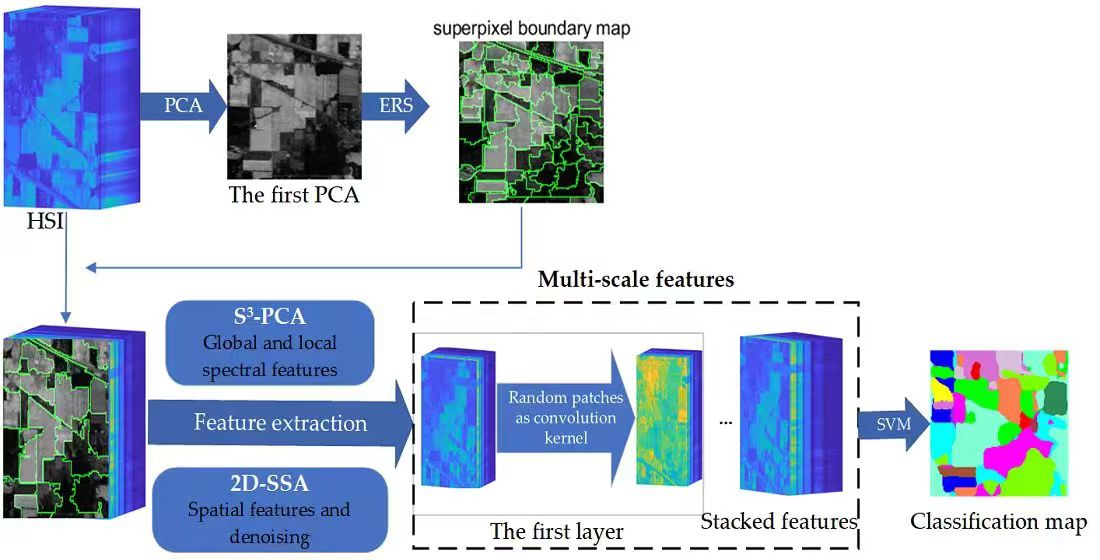
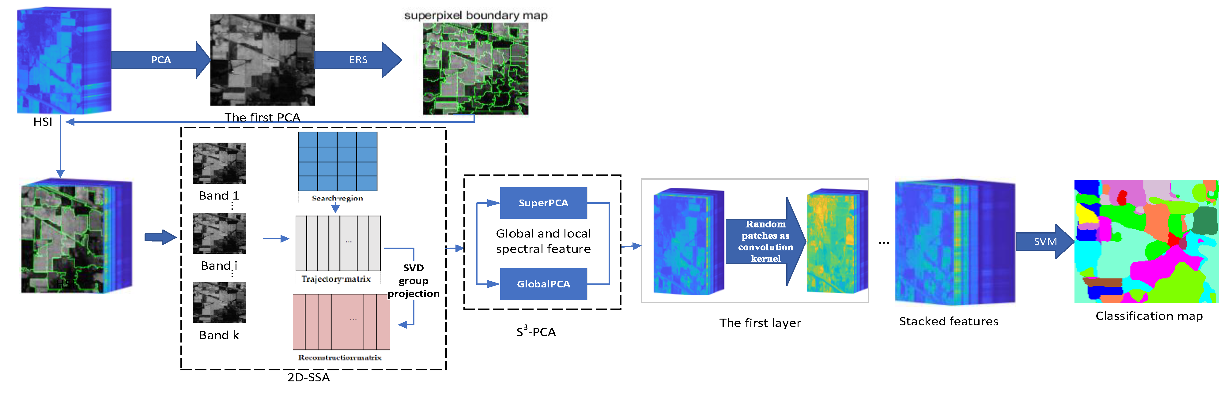
2.4. Proposed MS-RPNet Model

A central problem in hyperspectral image classification is spectral uncertainty, where spectral features alone cannot accurately and robustly identify a pixel point in a hyperspectral image. This motivates the need for recent spectral spatial classification methods to additionally consider spatial information and reduce the effect of spectral uncertainty, and then consider the noise-induced intra-class variation and higher inter-class similarity. This paper introduces a novel model called MS-RPNet (Figure 1) which uses 2D-SSA for noise removal and spatial feature extraction. Then, global and local features are separately extracted using superpixel-based S³-PCA, and the final features are obtained by random patch convolution and other steps according to the cascade structure of RPNet. The layered extraction superimposes the spatial difference information into multi-scale spatial features, which complements the features of various land covers. Finally, the final fusion features were classified by SVM to obtain the final classification results.

2.4.1. S³-PCA Domain Feature Extraction and Fusion with 2D-SSA

Let a hyperspectral cube be $D\in R^{D_x\times D_y\times D_{\lambda }}$, ${\mathrm{x}}_n={[x_{n1},x_{n2},\dots ,x_{n{D}_{\lambda }}]}^T$; $n\in [1,n]$, is the each pixel’s spectral vector, where the total number of pixels is $N=D_x{D}_y$. To avoid spectral distortion, the effective features of the homogeneous region are extracted by the superpixel segmentation technique. To reduce the computational effort of superpixel segmentation, the first principal component of HSI to be classified is denoted as $P{C}_1=R^{D_x\times D_y}$. This is first extracted by PCA, and then the entropy rate superpixel segmentation (ERS) [31] algorithm is used for superpixel segmentation of the first principal component to generate a homogeneous region block $P{C}_1={\displaystyle \underset{k=1}{\overset{s}{\cup }}{B}_k}$, where ($B_k\cap B_g=\varnothing \ne g$), S is the superpixel number and $B_k$ is the kth pixel. 2D-SSA is applied for noise removal and spatial feature extraction: first, an embedding window $L\in R^{L_x\times L_y}$ is cfreated; then, the trajectory matrix $T\in R^{\mathrm{m}\times n}$ is created, where $m=L_x\times L_y$, $n=(D_x-L_x+1)(D_y-D_y+1)$. For simplicity, we usually make $L_x=L_y$, and then SVD, grouping and diagonal averaging are used to obtain the reconstructed image Z. Based on the homogeneous regions formed by segmentation, the reconstructed image Z is subjected to the superpixel-based S³-PCA method to reduce the data dimensionality and obtain global–local spatial–spectral features $H=[H_{\mathrm{g}},H_l]\in R^{D_{\mathrm{x}}{D}_y\times \mathrm{p}}$ (where p is the principal component fraction), and the combined application of 2D-SSA and S³-PCA is a useful method to suppress the noise and strengthen the recognition of spectral space. Compared with the original HSI, the processed image has richer spectral diversity features and lower feature dimensionality.

2.4.2. Convolution with Random Patches

A whitening operation is performed on the reduced dimensional data H, which makes the variance in different bands similar and reduces the different correlation of the bands [39]. Then, k pixels are randomly selected from the data after the Whitening operation, and a block of size w × w × p is taken around each pixel, i.e., k random blocks are obtained. For the pixels distributed at the edges, the neighboring vacant pixels are filled by mirroring. Then, these k random blocks $P_1,P_2,\dots ,P_k$ are used as convolution kernels, and the convolution operation between $H_{Whitening}$ and random patches is performed to obtain k feature maps: $I_i:I_i={\displaystyle \sum _{j=1}^p{H}_{Whitening}{}^{(j)}}*P_i{}^{(j)}$, $i=1,2,\dots ,k$, where $*$ denotes the 2D convolution operation. The activation function is arranged to improve the sparsity of the features: $f(I)=\max (0,I-M)$, $M=[m_2\dots m_2]$, where $m_2\in R^{D_x{D}_{\mathrm{y}}\times 1}$ and M, respectively, denote the average vector and matrix in a two-dimensional space for k times replications. Eventually, the features in the first layer are expressed as $Z^{(1)}=f(I)\in R^{D_x{D}_y\times k}$. $Z^{(l-1)}\in R^{D_x{D}_y\times \mathrm{k}}$ is assumed to be the features of layer $(l-1)$, which is input again to extract features and obtain the lth-layer features $Z^l$, from which the features of the different layers can be obtained. Finally, all the features are passed through an SVM (with RFB kernel) classifier to predict the category labels and obtain the classification result map. This was obtained using the algorithm flow in Algorithm 1.

Algorithm 1. The proposed hyperspectral image classification algorithm.

Input: HSI image D, principal component number (PC_num), superpixel number (Pixel_num), layer number (Layernum). The first layer: (1) Apply 2D-SSA to D for spatial feature extraction and noise removal, and the reconstructed image Z is obtained. (2) A first principal component analysis of Z to obtain PC1. (3) Apply super-pixel segmentation algorithm ERS to PC1 for division into multiple homogeneous regions. (4) Apply S3-PCA to obtain the global–local spectral–spatial feature H. (5) Extract k random patches for convolution operation to obtain convolution features. (6) The other layers L (L ≤ Layernum): (7) Update the matrix while repeating steps 2–5 to obtain different features $C^L$. (8) Combine $C^1~C^L$ with the raw spectral data to form the final features and normalize them. (9) The final classification result is obtained by SVM for classification. Output: Classification accuracy and classification results

3. Experiments

To test the feasibility and validity of this approach, we chose three data sets as the test case, and PCA, SuperPCA, S³-PCA, PCA-2D-SSA, SuperPCA-2D-SSA, RPNet-5 [40], S³-PCA-RPNet, DMLSR [59], LeNet [40] and SSFTT [60] were used as the control groups. OA is the percent of pixels that are properly sorted, AA is the percent of correctly sorted elements in each class, and Kappa coefficient is obtained using the confusion matrix, which combines OA and AA. The experimental environment was Windows 10 with processor Intel (R) Core (TM) i5-8250U CPU @ 1.60GHz, 8GB of RAM, and NVIDIA GeForce MX 150 graphics card.

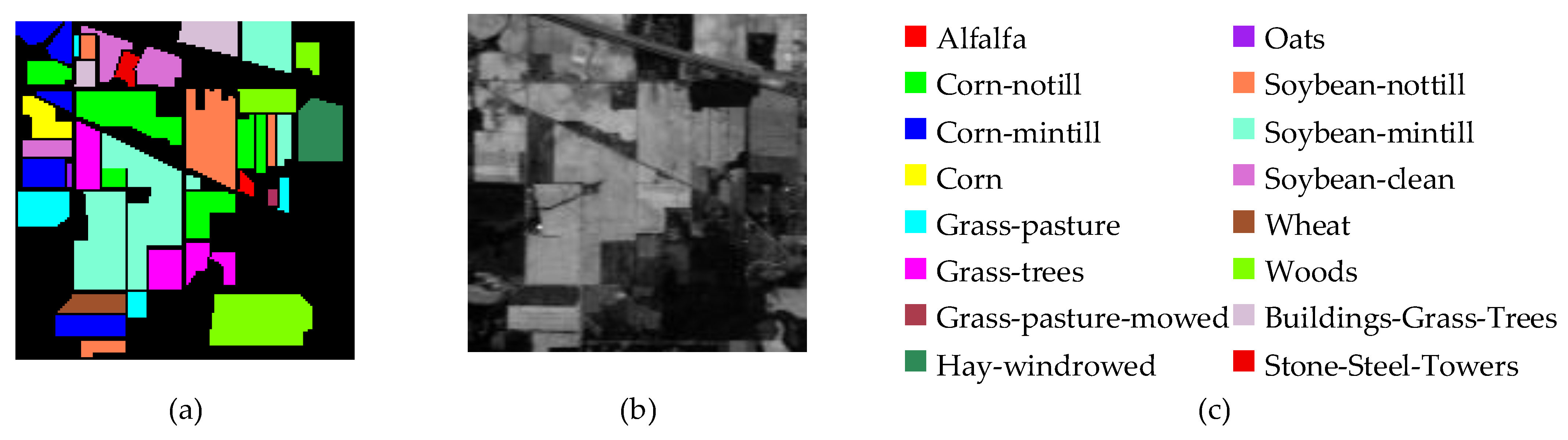
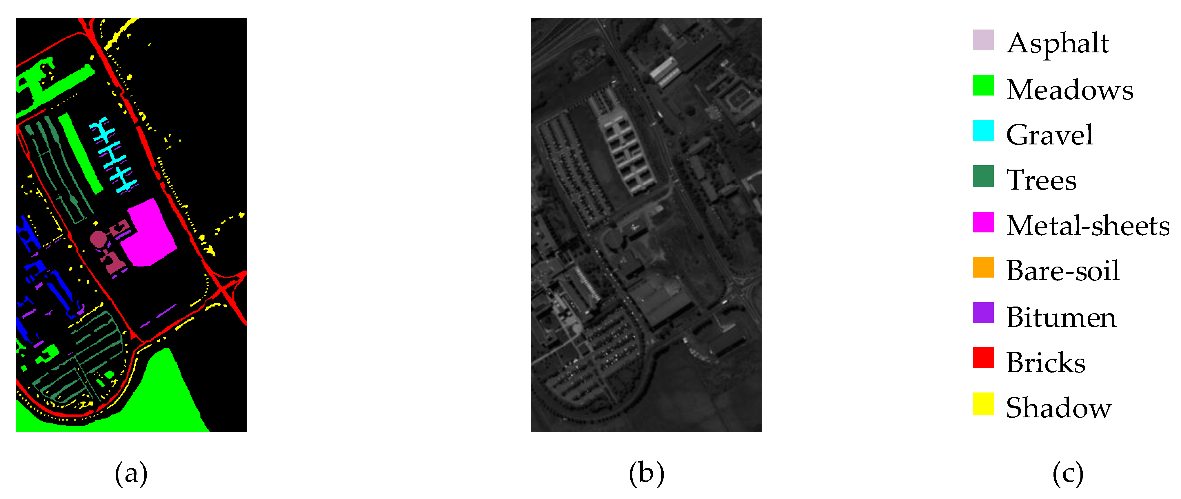
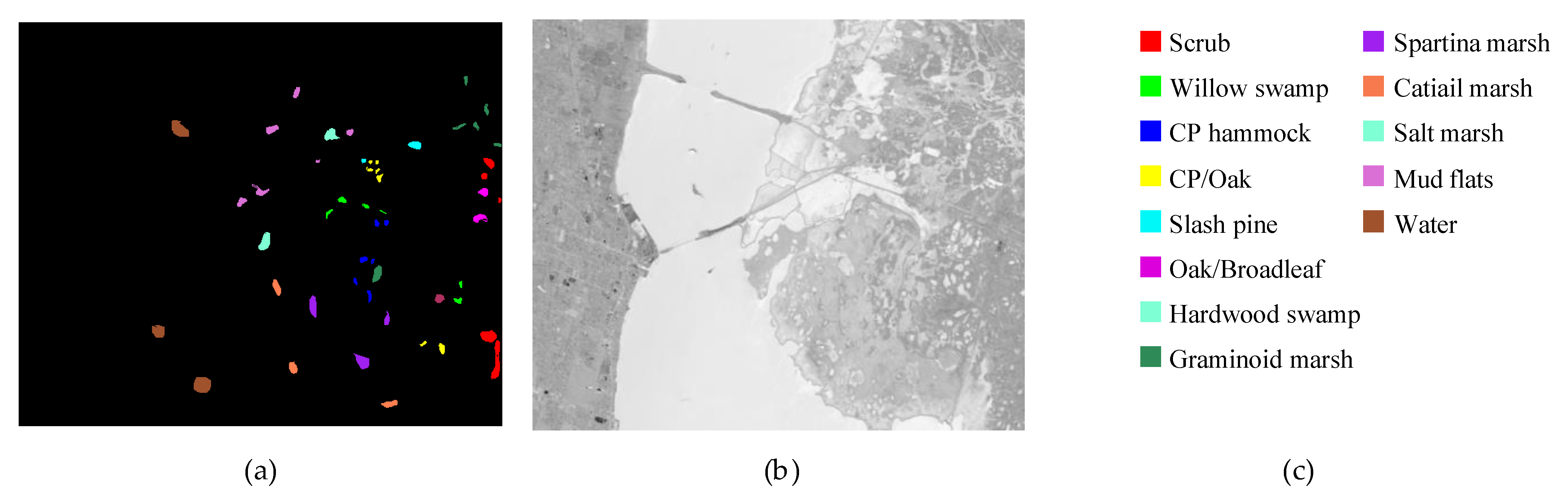
3.1. Introduction of Datasets

All experiments were conducted on the Indian Pines dataset, the KSC dataset and the Pavia University dataset. The real feature distribution and the first principal component of each original HSI are shown in Figure 2, Figure 3 and Figure 4. The Indian Pines datasets uses 200 bands after removing the bands covering the water-absorption region, which contain 16 types of feature elements. As for the KSC datasat, the discrimination of land cover according to its environment is difficult due to the similarity of spectral signatures for certain vegetation types. That is the reason that Figure 4b shows the fuzzy features of legend region in the ground-truth map to be different from those in Figure 2 and Figure 3b. More specific information can be found in

Table 1. Information about the three data sets.

Related Information	Data Sets
	Indian Pines	Pavia University	KSC
Sensor	AVIRIS	ROSIS	AVIRIS
Size (pixels)	145 × 145	610 × 340	512 × 614
Bands	200	103	176
Class	16	9	13
Spatial resolution (m)	20	1.3	18
Spectral wavelength (µm)	0.4–2.45	0.43–0.86	0.4–2.5

; the training and test sets are shown in

Table 2. Number of training and test samples used in Indian Pines dataset.

Class Number	Class Name	Training	Test
1	Alfalfa	30	16
2	Corn–notill	150	1278
3	Corn–mintill	150	680
4	Corn	100	137
5	Grass–pasture	150	333
6	Grass–trees	150	580
7	Grass–pasture–mowed	20	8
8	Hay–windrowed	150	328
9	Oats	15	5
10	Soybean–notill	150	822
11	Soybean–mintill	150	2305
12	Soybean–clean	150	443
13	Wheat	150	55
14	Woods	150	1115
15	Buildings–Grass–Trees–Drivers	50	336
16	Stone–Steel–Towers	50	43
	Total	1765	8484

,

Table 3. Number of training and test samples used in Pavia University dataset.

Class Number	Class Name	Training	Test
1	Asphalt	548	6083
2	Meadows	540	18,109
3	Gravel	392	1707
4	Trees	542	2522
5	Metal sheets	256	1089
6	Bare soil	532	4497
7	Bitumen	375	955
8	Bricks	514	3168
9	Shadows	231	716
	Total	3930	38,846

and

Table 4. Number of training and test samples used in KSC dataset.

Class Number	Class Name	Training	Test
1	Scrub	33	728
2	Willow swamp	23	220
3	CP hammock	24	232
4	CP/Oak	24	228
5	Slash pine	15	146
6	Oak/Broadleaf	22	207
7	Hardwood swamp	9	96
8	Graminoid marsh	38	393
9	Spartina marsh	51	469
10	Catiail marsh	39	365
11	Salt marsh	41	378
12	Mud flats	49	454
13	Water	91	836
	Total	459	4752

.

3.2. Parameter Analysis

In this experiment, there were several parameters that the influence classification results to different degrees. For instance, the random block size w and number k of model RPNet in the experiments were selected according to the literature [38], i.e., w = 21 and k = 20, $L_x\times L_y$ fixed at 10 × 10, and the rest of the parameter settings were shown in the following section. The data were repeated 10 times, and the mean was taken as the end result.

(1)

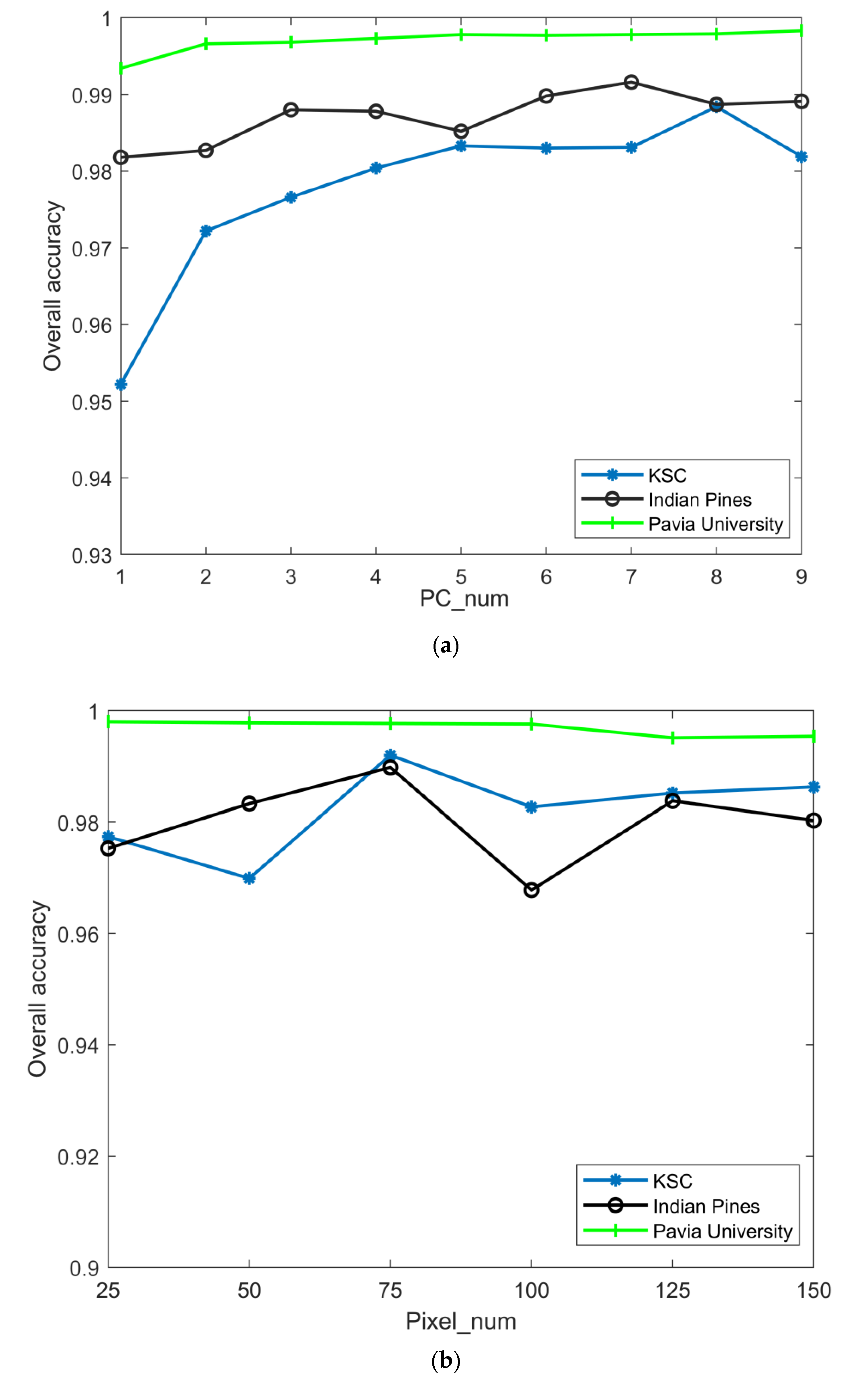
Analyze the effect of the parameter PC_num (number of principal components) on the experiment. The values of PC_num were divided into 9 cases (PC_num = 1, 2, 3, 4, 5, 6, 7, 8, 9), the effect of parameter PC_num on classification accuracy was observed in 9 cases, and the specific classification accuracy is plotted in Figure 5. From the figure, it can be seen that for the Indian Pines dataset, the variation in PCA does not affect the overall precision of classification, and the principal component dimension is taken as 7; for the Pavia University dataset, the change in the principal component dimension has a smaller impact on the overall accuracy, and the low-dimensional matrix is considered to be more beneficial to the subsequent calculation of the model, and PC_num = 5. For the KSC dataset, the change in the principal component dimension causes the overall accuracy to fluctuate, and the curves show a tendency to increase and then level, and PC_num = 8.

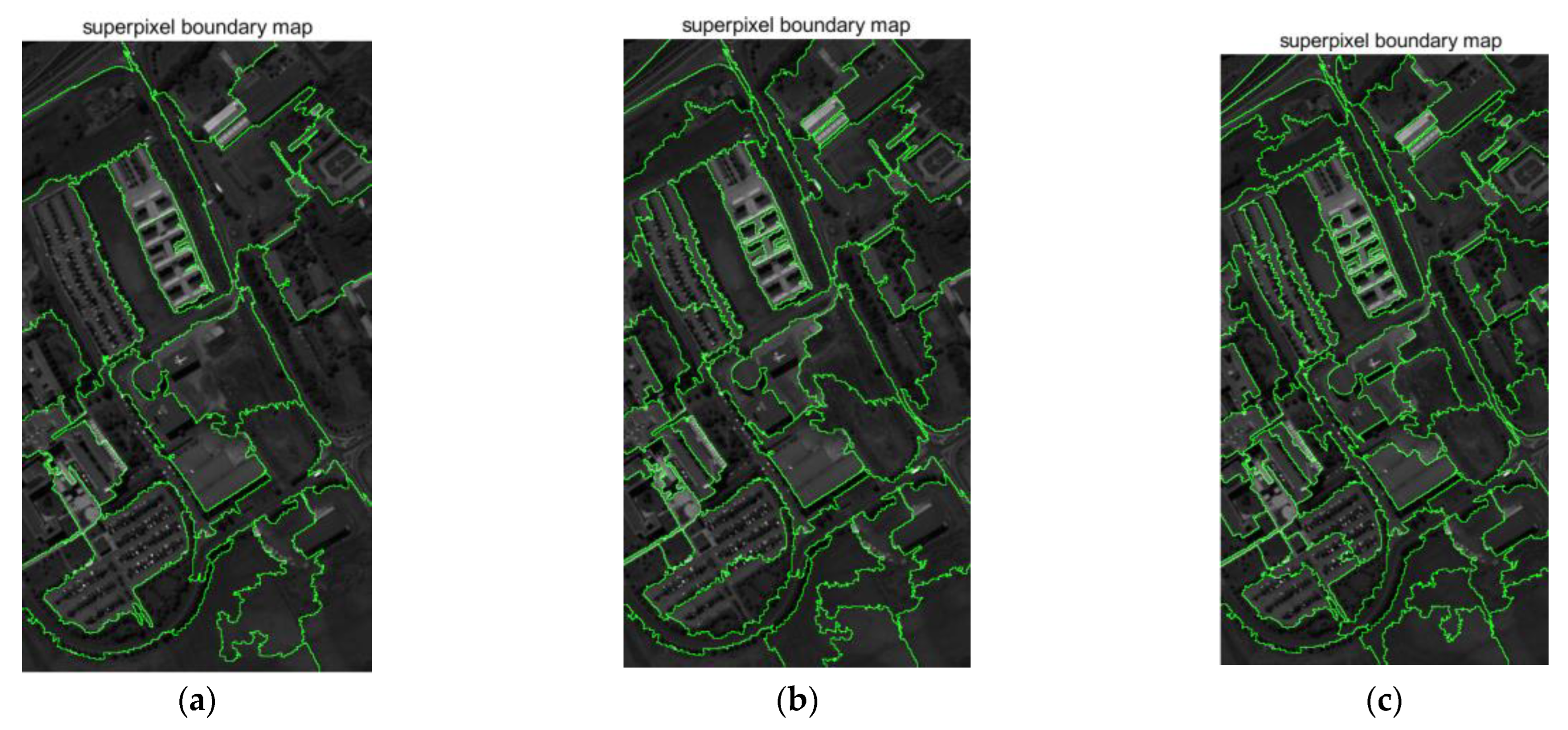
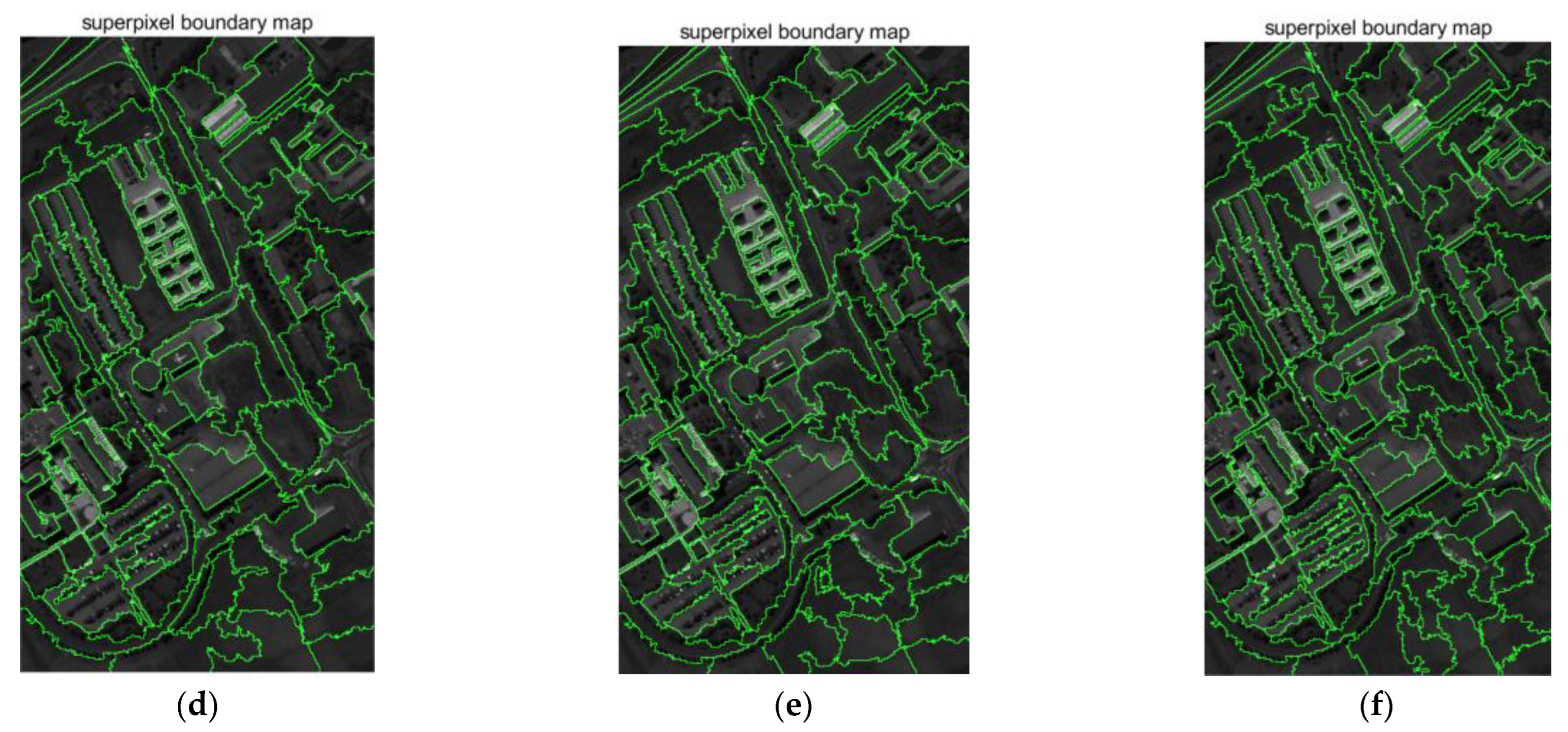
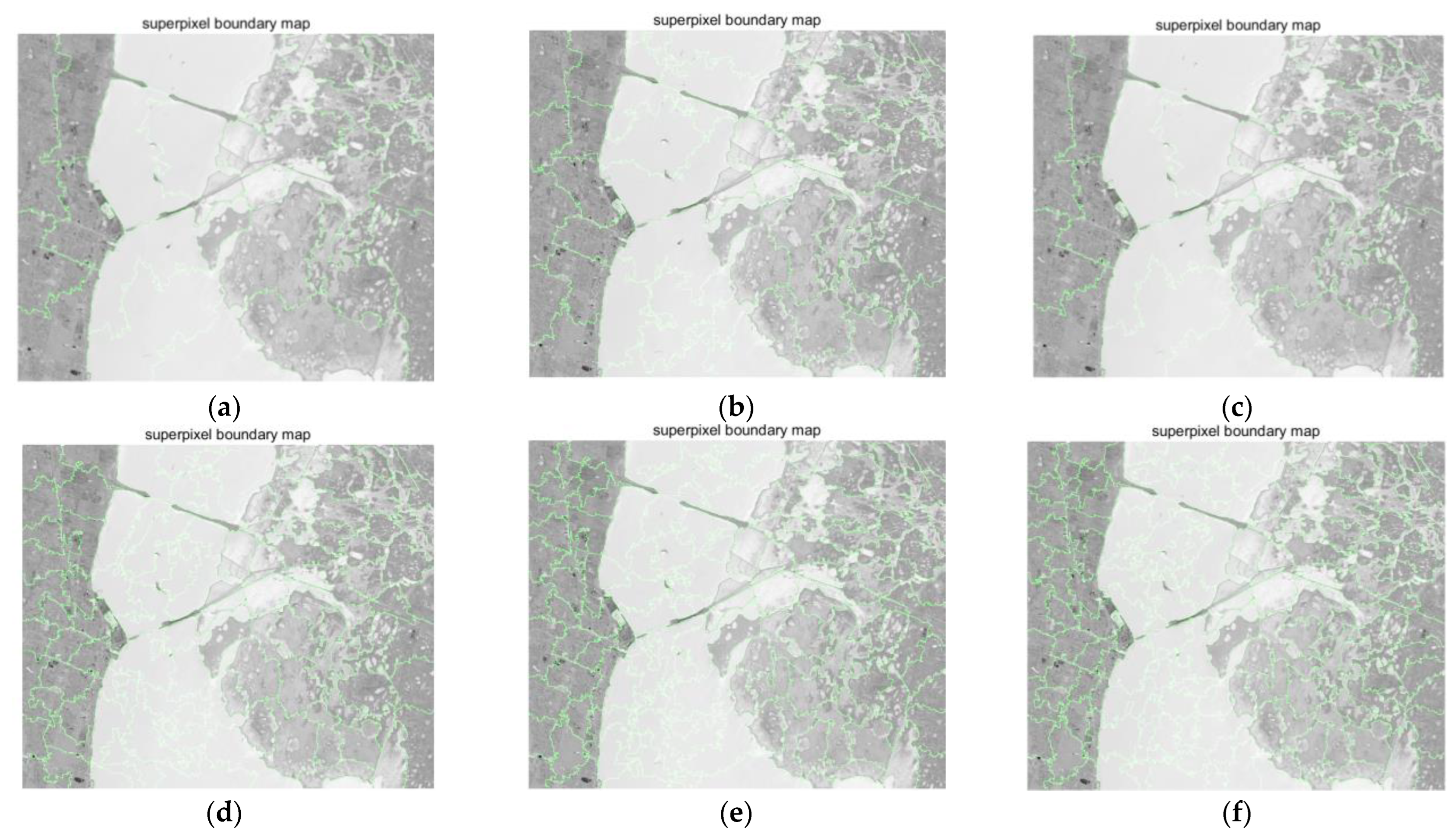
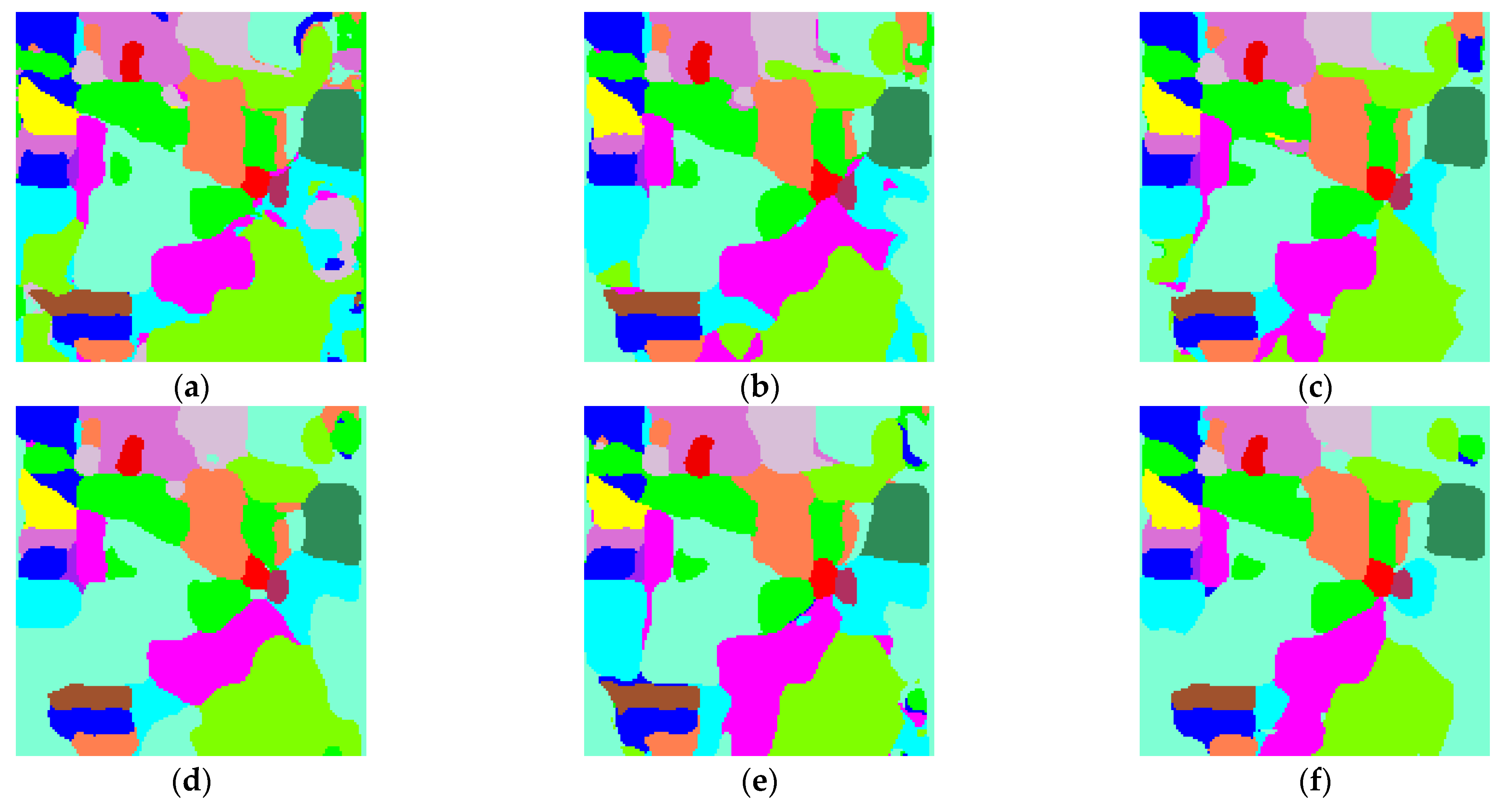
(2)

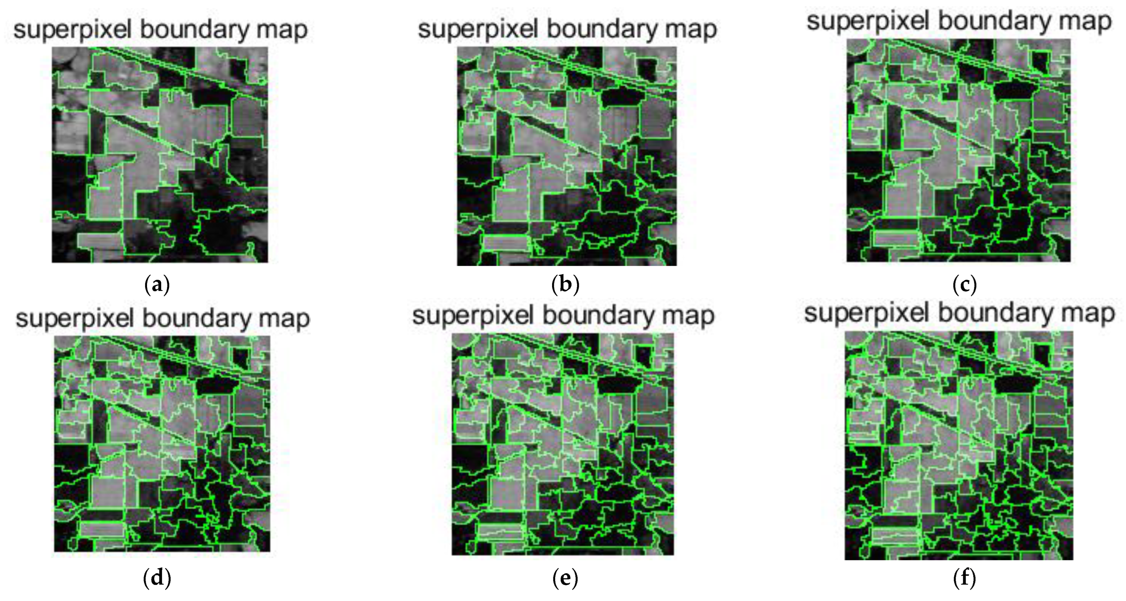
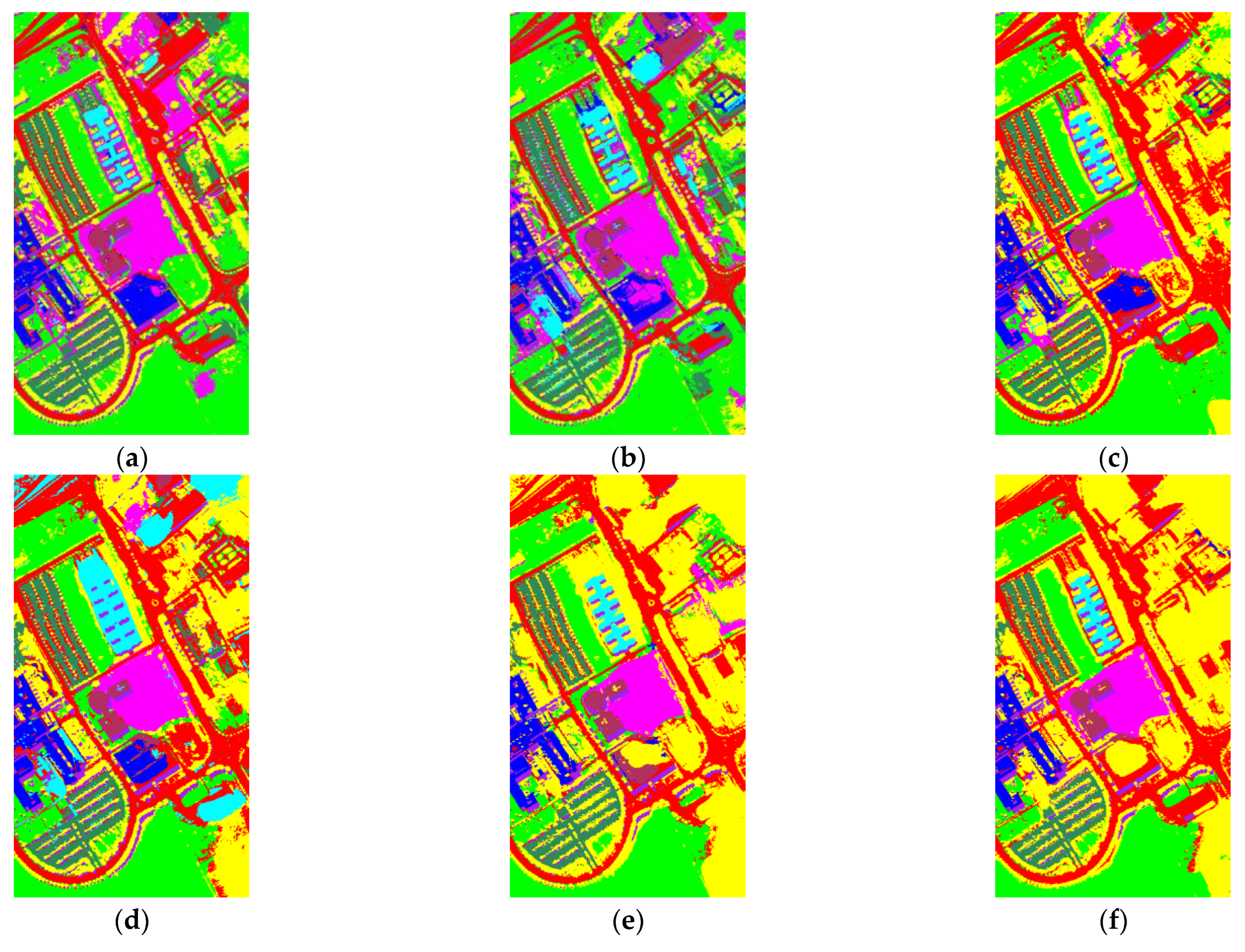
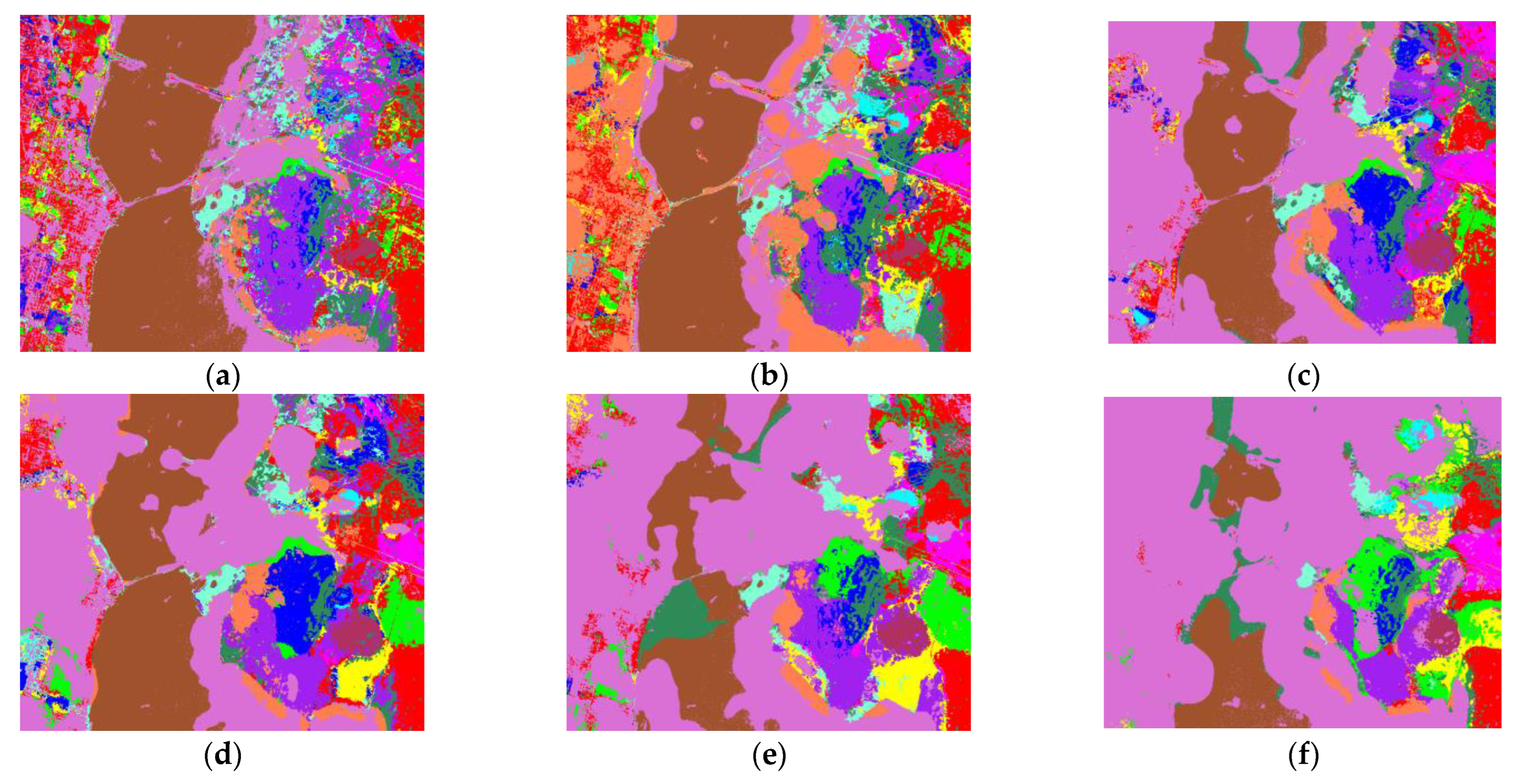
Analyze the effect of the parameter Pixel_num (superpixel number) on the experiment. The PC_nums are fixed according to the optimal number in (1). The specific superpixel segmentation graphs obtained by dividing the Pixel_num values into six cases (Pixel_num = 25, 50, 75, 100, 125, 150 are shown in Figure 6, Figure 7 and Figure 8. The number of superpixels determines the granularity of the segmentation result and various classification results. A larger number of superpixels produces finer-grained segmentation results that can better preserve the detailed image information, but may retain redundant information, while a smaller number of superpixels produces coarser segmentation results, but may lose some details. Thus, we need to choose this according to the specific application requirements and image characteristics. From Figure 5, it is obvious that different superpixel numbers make a greater difference to the classification accuracy for the first two datasets, which further indicates that the introduction of superpixel segmentation helps to improve classification accuracy. For the Pavia University dataset, the effect of the change in the number of superpixels on the overall accuracy is also not significant. An increase in the number of superpixels leads to an increase in the computational complexity of the algorithm. Considering the computational complexity, the parameter Pixel_num is set to Pixel_num = 75, and a high overall accuracy is achieved on the validation set of each dataset.

(3)

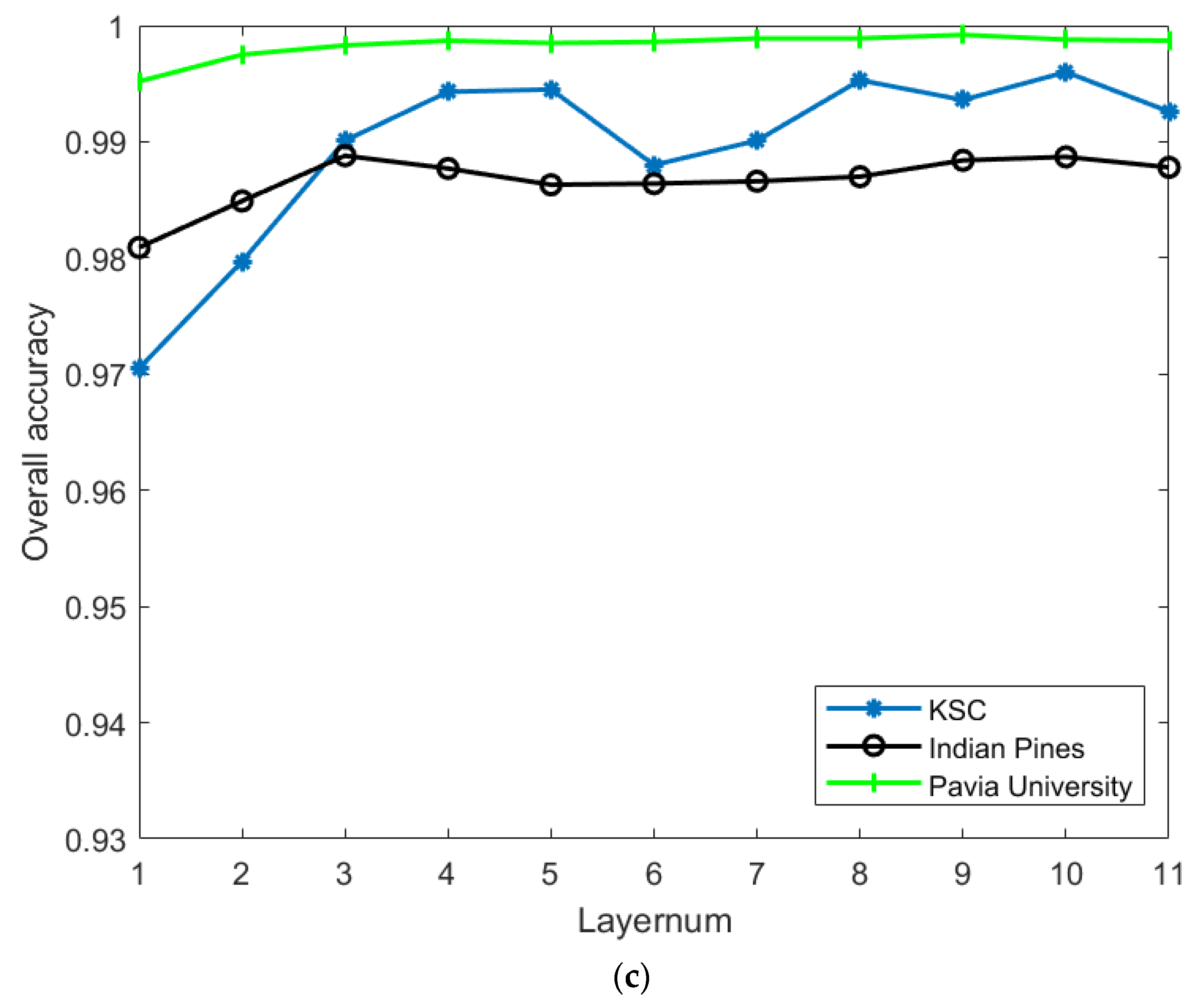
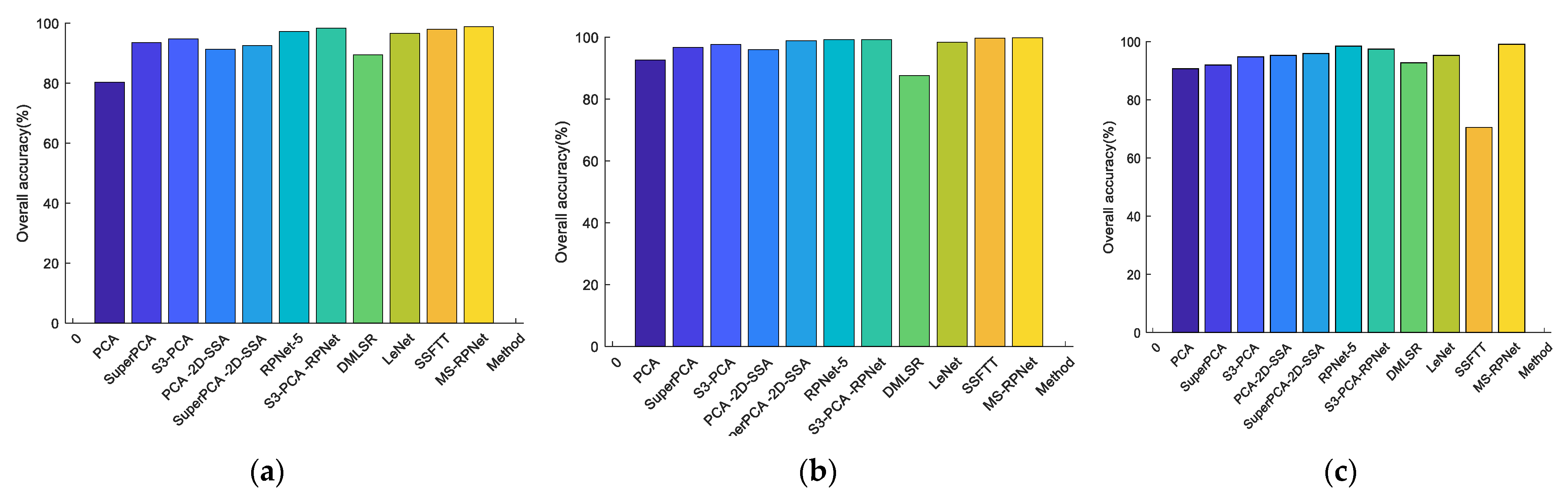
Analyze the effect of the parameter Layernum on the experiment. The PC_nums and pixel_nums are fixed according to the optimal number in (1). The classification results are shown in Figure 9, Figure 10 and Figure 11. The overall accuracy gradually increases and then stabilizes when the layer depth increases, which indicates that the random blocks extracted from the HSI contain useful information. However, an architecture that is too deep not only does not improve the accuracy, but also increases the computational complexity. According to Figure 5., the number of layers is taken as 3, 3, 5 respectively.

4. Discussion

This section compares the improvements proposed in this paper with PCA, SuperPCA, S³-PCA, PCA-2D-SSA, SuperPCA-2D-SSA, RPNet-5 [40], S³-PCA-RPNet, DMLSR [59], LeNet [40] and SSFTT [60] to assess the classification accuracy using support vector machines on the three data sets. The diagrams about classification accuracy are straightforwardly drawn in Figure 12, respectively, the classification results are shown in Figure 13, Figure 14 and Figure 15. From the control results in

Table 5. Classification result of the Indian Pines dataset.

Class	PCA	SuperPCA	S3-PCA	PCA -2D-SSA	SuperPCA -2D-SSA	RPNet-5	S3-PCA -RPNet	DMLSR	LeNet	SSFTT	Proposed
1	87.50	87.50	100	93.75	100	100	100	82.14	100	95.12	87.50
2	75.04	89.36	92.49	87.87	94.91	96.48	97.97	85.98	92.78	97.57	97.10
3	79.85	93.24	96.18	93.53	88.09	98.38	97.94	82.93	97.98	96.94	98.53
4	78.10	92.70	97.81	94.89	97.08	97.82	100	77.62	99.48	97.10	100
5	94.59	98.80	99.70	99.40	97.30	99.40	98.80	93.77	98.31	99.04	99.10
6	97.07	99.66	100	98.97	100	99.66	99.83	99.32	98.87	99.20	99.83
7	100	100	87.50	87.50	87.50	100	87.50	93.75	100	95.65	100
8	99.09	100	100	100	99.70	100	100	99.66	99.74	99.51	100
9	100	100	100	100	80.00	100	100	83.33	100	92.86	100
10	80.41	94.89	90.63	93.55	93.43	93.43	98.66	87.84	94.35	97.56	99.51
11	70.07	91.02	91.71	84.21	86.20	95.70	97.74	88.53	93.45	96.88	98.05
12	86.23	95.49	96.39	94.36	95.26	99.32	99.10	91.83	98.26	98.97	99.32
13	98.18	100	100	100	100	100	100	99.19	100	100	100
14	91.93	99.55	98.83	95.87	97.76	99.91	99.91	94.33	99.05	99.91	99.91
15	58.63	94.35	94.64	90.77	86.31	96.13	91.67	72.41	98.13	98.78	97.32
16	97.69	97.67	97.67	100	90.70	100	95.35	94.55	99.00	87.50	97.67
OA (%)	80.33	93.58	94.78	91.34	92.57	97.21	98.30	89.49	96.67	97.94	98.87
Kappa (%)	77.37	92.57	93.94	89.99	91.41	96.87	98.02	88.02	95.84	97.65	98.05

,

Table 6. Classification result of the Pavia University dataset.

Class	PCA	SuperPCA	S3-PCA	PCA -2D-SSA	SuperPCA -2D-SSA	RPNet-5	S3-PCA -RPNet	DMLSR	LeNet	SSFTT	Proposed
1	90.79	93.69	97.32	93.84	98.75	98.29	98.83	86.51	98.32	99.78	99.64
2	92.94	97.58	97.97	96.36	98.35	99.37	99.32	88.31	97.05	99.99	99.83
3	84.07	94.49	95.84	94.32	99.82	99.36	99.18	78.53	98.00	99.90	99.82
4	98.06	98.02	97.22	98.89	99.33	99.41	98.69	96.76	99.00	98.77	99.37
5	99.54	99.82	99.45	99.45	99.54	100	99.82	100	99.73	100	99.63
6	94.62	97.80	97.98	96.22	99.69	99.91	99.29	85.65	97.51	99.87	99.91
7	93.30	95.92	98.53	96.54	99.90	99.79	99.16	92.61	99.31	99.84	99.79
8	87.31	95.04	96.62	93.75	99.34	99.34	99.34	80.54	98.05	98.02	99.21
9	100	99.86	99.86	100	100	100	99.86	100	99.88	98.43	99.86
OA (%)	92.60	96.74	97.71	95.97	98.88	99.27	99.21	87.54	98.34	99.64	99.76
Kappa (%)	90.02	95.66	96.87	94.52	98.77	99.18	98.93	80.15	97.52	99.52	99.68

and

Table 7. Classification result of the KSC dataset.

Class	PCA	SuperPCA	S3-PCA	PCA -2D-SSA	SuperPCA -2D-SSA	RPNet-5	S3-PCA -RPNet	DMLSR	LeNet	SSFTT	Proposed
1	90.80	91.07	90.38	94.92	92.72	97.12	96.84	89.35	91.74	53.04	99.73
2	82.27	90.45	98.18	97.73	98.64	98.64	94.55	92.89	90.09	60.66	100
3	88.79	95.26	93.10	94.40	97.41	99.14	95.26	93.75	86.34	33.33	97.84
4	67.98	78.07	85.53	90.35	92.54	90.79	95.61	75.98	76.80	39.33	92.98
5	63.70	58.90	80.82	84.25	90.41	98.63	93.15	79.39	92.40	93.94	97.26
6	69.57	57.00	87.44	61.35	90.82	99.03	87.44	77.30	90.34	0	99.52
7	92.71	100	96.88	80.21	100	100	92.71	78.16	90.94	50.00	96.88
8	90.59	96.95	99.24	98.47	92.11	98.22	97.96	93.24	94.35	57.54	98.73
9	97.87	97.01	97.44	98.72	98.29	100	100	99.28	97.85	85.92	100
10	89.32	86.03	96.16	98.08	97.81	98.63	96.71	98.77	99.48	66.75	98.90
11	97.35	93.92	97.35	98.41	94.18	98.94	99.74	99.11	99.89	94.34	99.47
12	98.46	95.37	94.05	99.78	96.92	100	99.56	90.86	98.55	79.34	100
13	99.28	99.88	99.88	99.88	99.88	99.28	100	99.60	100	93.72	99.76
OA (%)	90.72	91.98	94.80	95.24	95.88	98.46	97.43	92.73	95.29	70.51	99.11
Kappa (%)	89.78	91.07	94.22	94.70	95.41	98.29	96.25	91.90	94.97	53.91	99.02

. PCA-2D-SSA and SuperPCA-2D-SSA consistently provide better classification results than PCA and SuperPCA only, while S³-PCA achieves a higher classification accuracy than PCA and SuperPCA based on superpixel local reconstruction. Thus, we are expected to add S³-PCA to the RPNet model to achieve higher classification accuracy. In contrast, the lack of spatial information leads PCA and SuperPCA to achieve lower classification accuracy in the benchmark test method. From the classification result plots presented in Figure 13, Figure 14 and Figure 15, misclassification and noise are shown to occur when only spectral features are used for classification, and these results indicate that the combination of spatial and spectral features is of great importance to HSI classification. Therefore, the S³-PCA-2D-SSA strategy used in this paper can fuse the advantages of both, and always obtains higher accuracy by utilizing local–global spectral spatial features while suppressing data noise. Compared with the original RPNet, the addition of S³-PCA-2D-SSA can achieve the best OA on the three datasets. For the Indian Pine dataset, the OA is improved by 1.66%, for the Pavia University dataset and the OA is improved by 99.76%, and for the KSC dataset, the OA is improved by 1.68% due to the combination of the introduction of superpixels, while 2D-SSA allows for the network to use not only shallow and deep feature extraction, but to effectively utilize spectral–spatial features, reducing information redundancy and loss. In the experiment, the LeNet [40] and SSFIT [60] are a highly accurate competitive approach to the Indian Pines and Pavia University dataset. However, their shortcomings lie in the over-smoothing phenomenon, especially in the KSC dataset, since it is difficult to distinguish land-cover environments with the similar spectral characteristics of some vegetation types. Therefore, the proposed model outperforms others in terms of validity. Finally, speaking of the complexity of the model, it is undeniable that its time complexity is higher than other control group algorithms, but its classification performance is better. However, it is worth nothing that superpixel-based analysis and global and local feature extraction take up part of the execution time. Thus, we will research how to adaptively obtain the downscaling and superpixel number parameters, and also attempt to establish a lightweight network to reduce the network complexity while keeping its performers.

5. Conclusions

In this paper, a fusion algorithm based on S³-PCA, 2D-SSA and RPNet is presented, in which global and local spectral features are sufficiently and separately extracted using superpixel-based S³-PCA, while noise removal and spatial feature extraction are carried out by 2D-SSA. Then, the spectral–spatial features are integrated into the cascade structure of RPNet to achieve shallow and deep convolution and remove the redundant fusion information. The layered extraction superimposes the spatial difference information into multi-scale spatial features, which complements the features of various land covers. It is experimentally verified that the improved method has a higher overall classification accuracy than the related comparison methods on the three open-source datasets. However, it should be noted that the parameters of S³-PCA downscaling and superpixel number are adjusted through a large number of experiments, which increases the computational cost. Thus, how to adaptively obtain the parameters and establish a lightweight network will be explored to improve computational costs.

References

1. Camps-Valls, G.; Tuia, D.; Bruzzone, L.; Benediktsson, J.A. Advances in Hyperspectral Image Classification: Earth Monitoring with Statistical Learning Methods. IEEE Signal Process. Mag. 2013, 31, 45–54. [Google Scholar] [CrossRef] [Green Version]
2. Matthews, M.W.; Bernard, S.; Evers-King, H.; Lain, L.R. Distinguishing cyanobacteria from algae in optically complex inland waters using a hyperspectral radiative transfer inversion algorithm. Remote Sens. Environ. 2020, 248, 111981. [Google Scholar] [CrossRef]
3. Carrino, T.A.; Crósta, A.P.; Toledo, C.L.B.; Silva, A.M. Hyperspectral remote sensing applied to mineral exploration in southern Peru: A multiple data integration approach in the Chapi Chiara gold prospect. Int. J. Appl. Earth Obs. Geoinf. 2018, 64, 287–300. [Google Scholar] [CrossRef]
4. Tong, X.Y.; Xia, G.S.; Lu, Q.; Shen, H.; Li, S.; You, S.; Zhang, L. Land-cover classification with high-resolution remote sensing images using transferable deep models. Remote Sens. Environ. 2020, 237, 111322. [Google Scholar] [CrossRef] [Green Version]
5. Ma, W.; Gong, C.; Hu, Y.; Meng, P.; Xu, F. The Hughes phenomenon in hyperspectral classification based on the ground spectrum of grasslands in the region around Qinghai Lake. In International Symposium on Photoelectronic Detection and Imaging 2013: Imaging Spectrometer Technologies and Applications; SPIE: Bellingham, WA, USA, 2013; Volume 8910, pp. 363–373. [Google Scholar]
6. Du, Q.; Yang, H. Similarity-Based Unsupervised Band Selection for Hyperspectral Image Analysis. IEEE Geosci. Remote Sens. Lett. 2008, 5, 564–568. [Google Scholar] [CrossRef]
7. Yang, H.; Du, Q.; Chen, G. Unsupervised hyperspectral band selection using graphics processing units. IEEE J. Sel. Top. Appl. Earth Obs. Remote Sens. 2011, 4, 660–668. [Google Scholar] [CrossRef]
8. Wang, Q.; Lin, J.; Yuan, Y. Salient Band Selection for Hyperspectral Image Classification via Manifold Ranking. IEEE Trans. Neural Netw. Learn. Syst. 2016, 27, 1279–1289. [Google Scholar] [CrossRef]
9. Jia, S.; Tang, G.; Zhu, J.; Li, Q. A Novel Ranking-Based Clustering Approach for Hyperspectral Band Selection. IEEE Trans. Geosci. Remote Sens. 2015, 54, 88–102. [Google Scholar] [CrossRef]
10. Bruce, L.; Koger, C.; Li, J. Dimensionality reduction of hyperspectral data using discrete wavelet transform feature extraction. IEEE Trans. Geosci. Remote Sens. 2002, 40, 2331–2338. [Google Scholar] [CrossRef]
11. Zhao, W.; Du, S. Spectral–Spatial Feature Extraction for Hyperspectral Image Classification: A Dimension Reduction and Deep Learning Approach. IEEE Trans. Geosci. Remote Sens. 2016, 54, 4544–4554. [Google Scholar] [CrossRef]
12. Prasad, S.; Bruce, L.M. Limitations of Principal Components Analysis for Hyperspectral Target Recognition. IEEE Geosci. Remote Sens. Lett. 2008, 5, 625–629. [Google Scholar] [CrossRef]
13. Bandos, T.V.; Bruzzone, L.; Camps-Valls, G. Classification of Hyperspectral Images With Regularized Linear Discriminant Analysis. IEEE Trans. Geosci. Remote Sens. 2009, 47, 862–873. [Google Scholar] [CrossRef]
14. Lixin, G.; Weixin, X.; Jihong, P. Segmented minimum noise fraction transformation for efficient feature extraction of hyperspectral images. Pattern Recognit. 2015, 48, 3216–3226. [Google Scholar] [CrossRef]
15. Zabalza, J.; Ren, J.; Ren, J.; Liu, Z.; Marshall, S. Structured covariance principal component analysis for real-time onsite feature extraction and dimensionality reduction in hyperspectral imaging. Appl. Opt. 2014, 53, 4440–4449. [Google Scholar] [CrossRef] [Green Version]
16. Jia, X.; Richards, J.A. Segmented principal components transformation for efficient hyperspectral remote-sensing image display and classification. IEEE Trans. Geosci. Remote Sens. 1999, 37, 538–542. [Google Scholar] [CrossRef] [Green Version]
17. Zabalza, J.; Ren, J.; Yang, M.; Zhang, Y.; Wang, J.; Marshall, S.; Han, J. Novel Folded-PCA for improved feature extraction and data reduction with hyperspectral imaging and SAR in remote sensing. ISPRS J. Photogramm. Remote Sens. 2014, 93, 112–122. [Google Scholar] [CrossRef] [Green Version]
18. Zhang, H.; Li, J.; Huang, Y.; Zhang, L. A Nonlocal Weighted Joint Sparse Representation Classification Method for Hyperspectral Imagery. IEEE J. Sel. Top. Appl. Earth Obs. Remote Sens. 2013, 7, 2056–2065. [Google Scholar] [CrossRef]
19. Jiang, J.; Ma, J.; Chen, C.; Wang, Z.; Cai, Z.; Wang, L. SuperPCA: A Superpixelwise PCA Approach for Unsupervised Feature Extraction of Hyperspectral Imagery. IEEE Trans. Geosci. Remote Sens. 2018, 56, 4581–4593. [Google Scholar] [CrossRef] [Green Version]
20. Zhang, X.; Jiang, X.; Jiang, J.; Zhang, Y.; Liu, X.; Cai, Z. Spectral–Spatial and Superpixelwise PCA for Unsupervised Feature Extraction of Hyperspectral Imagery. IEEE Trans. Geosci. Remote Sens. 2021, 60, 5502210. [Google Scholar] [CrossRef]
21. Donoho, D.L. High-dimensional data analysis: The curses and blessings of dimensionality. AMS Math Chall. Lect. 2000, 1, 32. [Google Scholar]
22. Zhang, L.; Zhang, L.; Tao, D.; Huang, X. On combining multiple features for hyperspectral remote sensing image classification. IEEE Trans. Geosci. Remote Sens. 2011, 50, 879–893. [Google Scholar] [CrossRef]
23. Fauvel, M.; Tarabalka, Y.; Benediktsson, J.A.; Chanussot, J.; Tilton, J.C. Advances in spectral-spatial classification of hyperspectral images. Proc. IEEE 2013, 101, 652–675. [Google Scholar] [CrossRef]
24. Bao, R.; Xia, J.; Mura, M.D.; Du, P.; Chanussot, J.; Ren, J. Combining Morphological Attribute Profiles via an Ensemble Method for Hyperspectral Image Classification. IEEE Geosci. Remote Sens. Lett. 2016, 13, 359–363. [Google Scholar] [CrossRef]
25. Gu, Y.; Liu, T.; Jia, X.; Benediktsson, J.A.; Chanussot, J. Nonlinear Multiple Kernel Learning With Multiple-Structure-Element Extended Morphological Profiles for Hyperspectral Image Classification. IEEE Trans. Geosci. Remote Sens. 2016, 54, 3235–3247. [Google Scholar] [CrossRef]
26. Xia, J.; Mura, M.D.; Chanussot, J.; Du, P.; He, X. Random Subspace Ensembles for Hyperspectral Image Classification With Extended Morphological Attribute Profiles. IEEE Trans. Geosci. Remote Sens. 2015, 53, 4768–4786. [Google Scholar] [CrossRef]
27. Zabalza, J.; Ren, J.; Wang, Z.; Marshall, S.; Wang, J. Singular Spectrum Analysis for Effective Feature Extraction in Hyperspectral Imaging. IEEE Geosci. Remote Sens. Lett. 2014, 11, 1886–1890. [Google Scholar] [CrossRef] [Green Version]
28. Qiao, T.; Ren, J.; Wang, Z.; Zabalza, J.; Sun, M.; Zhao, H.; Li, S.; Benediktsson, J.A.; Dai, Q.; Marshall, S. Effective Denoising and Classification of Hyperspectral Images Using Curvelet Transform and Singular Spectrum Analysis. IEEE Trans. Geosci. Remote Sens. 2016, 55, 119–133. [Google Scholar] [CrossRef] [Green Version]
29. Zabalza, J.; Ren, J.; Zheng, J.; Han, J.; Zhao, H.; Li, S.; Marshall, S. Novel Two-Dimensional Singular Spectrum Analysis for Effective Feature Extraction and Data Classification in Hyperspectral Imaging. IEEE Trans. Geosci. Remote Sens. 2015, 53, 4418–4433. [Google Scholar] [CrossRef] [Green Version]
30. Yan, Y.; Ren, J.; Liu, Q.; Zhao, H.; Sun, H.; Zabalza, J. PCA-Domain Fused Singular Spectral Analysis for Fast and Noise-Robust Spectral–Spatial Feature Mining in Hyperspectral Classification. IEEE Geosci. Remote Sens. Lett. 2021, 20, 5505405. [Google Scholar] [CrossRef]
31. Fukushima, K. Neocognitron: A self-organizing neural network model for a mechanism of pattern recognition unaffected by shift in position. Biol. Cybern. 1980, 36, 193–202. [Google Scholar] [CrossRef]
32. Bengio, Y.; Lamblin, P.; Popovici, D.; Larochelle, H. Greedy layer-wise training of deep networks. In Proceedings of the Advances in Neural Information Processing Systems 19 (NIPS 2006), Vancouver, BC, Canada, 4–7 December 2006. [Google Scholar]
33. Hinton, G.E.; Osindero, S.; Teh, Y.-W. A Fast Learning Algorithm for Deep Belief Nets. Neural Comput. 2006, 18, 1527–1554. [Google Scholar] [CrossRef] [PubMed]
34. Yang, J.; Xiao, L.; Zhao, Y.Q.; Chan, J.C. Variational regularization network with attentive deep prior for hyperspectral–multispectral image fusion. IEEE Trans. Geosci. Remote Sens. 2021, 60, 5508817. [Google Scholar] [CrossRef]
35. Li, X.; Ding, M.; Gu, Y.; Pižurica, A. An End-to-End Framework for Joint Denoising and Classification of Hyperspectral Images. IEEE Trans. Neural Netw. Learn. Syst. 2023, 1–15. [Google Scholar] [CrossRef]
36. Xue, J.; Zhao, Y.; Huang, S.; Liao, W.; Chan, J.C.-W.; Kong, S.G. Multilayer Sparsity-Based Tensor Decomposition for Low-Rank Tensor Completion. IEEE Trans. Neural Netw. Learn. Syst. 2021, 33, 6916–6930. [Google Scholar] [CrossRef] [PubMed]
37. Zeng, H.; Xue, J.; Luong, H.Q.; Philips, W. Multimodal Core Tensor Factorization and Its Applications to Low-Rank Tensor Completion. IEEE Trans. Multimed. 2022, 1–15. [Google Scholar] [CrossRef]
38. Yang, J.; Xiao, L.; Zhao, Y.-Q.; Chan, J.C.-W. Unsupervised Deep Tensor Network for Hyperspectral–Multispectral Image Fusion. IEEE Trans. Neural Netw. Learn. Syst. 2023, 1–15. [Google Scholar] [CrossRef]
39. Chen, Y.; Zhao, X.; Jia, X. Spectral–Spatial Classification of Hyperspectral Data Based on Deep Belief Network. IEEE J. Sel. Top. Appl. Earth Obs. Remote Sens. 2015, 8, 2381–2392. [Google Scholar] [CrossRef]
40. Xu, Y.; Du, B.; Zhang, F.; Zhang, L. Hyperspectral image classification via a random patches network. ISPRS J. Photogramm. Remote Sens. 2018, 142, 344–357. [Google Scholar] [CrossRef]
41. Hong, D.; Han, Z.; Yao, J.; Gao, L.; Zhang, B.; Plaza, A.; Chanussot, J. SpectralFormer: Rethinking Hyperspectral Image Classification With Transformers. IEEE Trans. Geosci. Remote Sens. 2021, 60, 5518615. [Google Scholar] [CrossRef]
42. Zhou, X.; Cai, X.; Zhang, H.; Zhang, Z.; Jin, T.; Chen, H.; Deng, W. Multi-strategy competitive-cooperative co-evolutionary algorithm and its application. Inf. Sci. 2023, 635, 328–344. [Google Scholar] [CrossRef]
43. Li, M.; Zhang, W.; Hu, B.; Kang, J.; Wang, Y.; Lu, S. Automatic Assessment of Depression and Anxiety through Encoding Pupil-wave from HCI in VR Scenes. ACM Trans. Multimed. Comput. Commun. Appl. 2022. [Google Scholar] [CrossRef]
44. Sun, Q.; Zhang, M.; Zhou, L.; Garme, K.; Burman, M. A machine learning-based method for prediction of ship performance in ice: Part I. ice resistance. Mar. Struct. 2022, 83, 103181. [Google Scholar] [CrossRef]
45. Duan, Z.; Song, P.; Yang, C.; Deng, L.; Jiang, Y.; Deng, F.; Jiang, X.; Chen, Y.; Yang, G.; Ma, Y.; et al. The impact of hyperglycaemic crisis episodes on long-term outcomes for inpatients presenting with acute organ injury: A prospective, multicentre follow-up study. Front. Endocrinol. 2022, 13, 1057089. [Google Scholar] [CrossRef]
46. Xie, C.; Zhou, L.; Ding, S.; Liu, R.; Zheng, S. Experimental and numerical investigation on self-propulsion performance of polar merchant ship in brash ice channel. Ocean Eng. 2023, 269, 113424. [Google Scholar] [CrossRef]
47. Chen, T.; Song, P.; He, M.; Rui, S.; Duan, X.; Ma, Y.; Armstrong, D.G.; Deng, W. Sphingosine-1-phosphate derived from PRP-Exos promotes angiogenesis in diabetic wound healing via the S1PR1/AKT/FN1 signalling pathway. Burn. Trauma 2023, 11, tkad003. [Google Scholar] [CrossRef]
48. Ren, Z.; Zhen, X.; Jiang, Z.; Gao, Z.; Li, Y.; Shi, W. Underactuated control and analysis of single blade installation using a jackup installation vessel and active tugger line force control. Mar. Struct. 2023, 88, 103338. [Google Scholar] [CrossRef]
49. Chen, M.; Shao, H.; Dou, H.; Li, W.; Liu, B. Data Augmentation and Intelligent Fault Diagnosis of Planetary Gearbox Using ILoFGAN Under Extremely Limited Samples. IEEE Trans. Reliab. 2022, 1–9. [Google Scholar] [CrossRef]
50. Song, Y.; Zhao, G.; Zhang, B.; Chen, H.; Deng, W.; Deng, W. An enhanced distributed differential evolution algorithm for portfolio optimization problems. Eng. Appl. Artif. Intell. 2023, 121, 106004. [Google Scholar] [CrossRef]
51. Yan, S.; Shao, H.; Min, Z.; Peng, J.; Cai, B.; Liu, B. FGDAE: A new machinery anomaly detection method towards complex operating conditions. Reliab. Eng. Syst. Saf. 2023, 236, 109319. [Google Scholar] [CrossRef]
52. Li, M.; Zhang, J.; Song, J.; Li, Z.; Lu, S. A Clinical-Oriented Non-Severe Depression Diagnosis Method Based on Cognitive Behavior of Emotional Conflict. IEEE Trans. Comput. Soc. Syst. 2022, 10, 131–141. [Google Scholar] [CrossRef]
53. Cai, J.; Ding, S.; Zhang, Q.; Liu, R.; Zeng, D.; Zhou, L. Broken ice circumferential crack estimation via image techniques. Ocean Eng. 2022, 259, 111735. [Google Scholar] [CrossRef]
54. Yu, Y.; Tang, K.; Liu, Y. A Fine-Tuning Based Approach for Daily Activity Recognition between Smart Homes. Appl. Sci. 2023, 13, 5706. [Google Scholar] [CrossRef]
55. Lin, J.; Shao, H.; Zhou, X.; Cai, B.; Liu, B. Generalized MAML for few-shot cross-domain fault diagnosis of bearing driven by heterogeneous signals. Expert Syst. Appl. 2023, 230, 120696. [Google Scholar] [CrossRef]
56. Huang, C.; Zhou, X.; Ran, X.; Wang, J.; Chen, H.; Deng, W. Adaptive cylinder vector particle swarm optimization with differential evolution for UAV path planning. Eng. Appl. Artif. Intell. 2023, 121, 105942. [Google Scholar] [CrossRef]
57. Chen, X.; Shao, H.; Xiao, Y.; Yan, S.; Cai, B.; Liu, B. Collaborative fault diagnosis of rotating machinery via dual adversarial guided unsupervised multi-domain adaptation network. Mech. Syst. Signal Process. 2023, 198, 1104270. [Google Scholar] [CrossRef]
58. Caywood, M.S.; Willmore, B.; Tolhurst, D.J. Independent Components of Color Natural Scenes Resemble V1 Neurons in Their Spatial and Color Tuning. J. Neurophysiol. 2004, 91, 2859–2873. [Google Scholar] [CrossRef] [Green Version]
59. Zhang, Y.; Li, W.; Li, H.-C.; Tao, R.; Du, Q. Discriminative Marginalized Least-Squares Regression for Hyperspectral Image Classification. IEEE Trans. Geosci. Remote Sens. 2019, 58, 3148–3161. [Google Scholar] [CrossRef]
60. Sun, L.; Zhao, G.; Zheng, Y.; Wu, Z. Spectral–spatial feature tokenization transformer for hyperspectral image classification. IEEE Trans. Geosci. Remote Sens. 2022, 60, 5522214. [Google Scholar] [CrossRef]
Figure 1. The flow chart of the proposed MS-RPNet model.
Remotesensing 15 03402 g001
Figure 2. Indian Pines dataset: (a) ground-truth map; (b) the first principal component; (c) legend.
Remotesensing 15 03402 g002
Figure 3. Pavia University dataset: (a) ground-truth map; (b) the first principal component; (c) legend.
Remotesensing 15 03402 g003
Figure 4. KSC dataset: (a) ground-truth map; (b) the first principal component; (c) legend.
Remotesensing 15 03402 g004
Figure 5. The overall accuracy with different parameters: (a) number of principal components; (b) number of superpixels; (c) number of layers.
Remotesensing 15 03402 g005aRemotesensing 15 03402 g005b
Figure 6. Segmentation map with different number superpixels for the Indian Pines dataset: (a) pixel_num = 25; (b) pixel_num = 50; (c) pixel_num = 75; (d) pixel_num = 100; (e) pixel_num = 125; (f) pixel_num = 150.
Remotesensing 15 03402 g006
Figure 7. Segmentation map with different number superpixels for the Pavia University dataset: (a) pixel_num = 25; (b) pixel_num = 50; (c) pixel_num = 75; (d) pixel_num = 100; (e) pixel_num = 125; (f) pixel_num = 150.
Remotesensing 15 03402 g007aRemotesensing 15 03402 g007b
Figure 8. Segmentation map with different number superpixels for the KSC dataset: (a) pixel_num = 25; (b) pixel_num = 50; (c) pixel_num = 75; (d) pixel_num = 100; (e) pixel_num = 125; (f) pixel_num = 150.
Remotesensing 15 03402 g008
Figure 9. The classification maps with different numbers of layer for the Indian Pines dataset: (a) layernum = 1; (b) layernum = 3; (c) layernum = 5; (d) layernum = 7; (e) layernum = 9; (f) layernum = 11.
Remotesensing 15 03402 g009
Figure 10. The classification maps with different numbers of layer for the Pavia University dataset: (a) layernum = 1; (b) layernum = 3; (c) layernum = 5; (d) layernum = 7; (e) layernum = 9; (f) layernum = 11.
Remotesensing 15 03402 g010
Figure 11. The classification maps with different numbers of layer for the KSC dataset: (a) layernum = 1; (b) layernum = 3; (c) layernum = 5; (d) layernum = 7; (e) layernum = 9; (f) layernum = 11.
Remotesensing 15 03402 g011
Figure 12. The comparison of different methods’ accuracy: (a) Indian Pine dataset; (b) Pavia University dataset; (c) the KSC dataset.
Remotesensing 15 03402 g012
Figure 13. The classification maps with different methods for the Indian Pine dataset: (a) truth; (b) PCA; (c) SuperPCA; (d) S3-PCA; (e) PCA-2D-SSA; (f) SuperPCA-2D-SSA; (g) S3-PCA-RPNet (h) RPNet-5; (i) DMLSR; (j) LeNet; (k) SSFTT; (l) Proposed.
Remotesensing 15 03402 g013
Figure 14. The classification maps with different methods for the Pavia University dataset: (a) truth; (b) PCA; (c) SuperPCA; (d) S3-PCA; (e) PCA-2D-SSA; (f) SuperPCA-2D-SSA; (g) S3-PCA-RPNet (h) RPNet-5; (i) DMLSR; (j) LeNet; (k) SSFTT; (l) Proposed.
Remotesensing 15 03402 g014
Figure 15. The classification maps with different methods for the KSC dataset: (a) truth; (b) PCA; (c) SuperPCA; (d) S3-PCA; (e) PCA-2D-SSA; (f) SuperPCA-2D-SSA; (g) S3-PCA-RPNet (h) RPNet-5; (i) DMLSR; (j) LeNet; (k) SSFTT; (l) Proposed.
Remotesensing 15 03402 g015aRemotesensing 15 03402 g015b