Soil Moisture Retrieval Using GNSS-IR Based on Empirical Modal Decomposition and Cross-Correlation Satellite Selection

Abstract

Global Navigation Satellite System interferometric reflectometry (GNSS-IR), as a new remote sensing detection technology, can retrieve surface soil moisture (SM) by separating the modulation terms from the effective signal-to-noise ratio (SNR) data. However, traditional low-order polynomials are prone to over-fitting when separating modulation terms. Moreover, the existing research mainly relies on prior information to select satellites for SM retrieval. Accordingly, this study proposes a method based on empirical modal decomposition (EMD) and cross-correlation satellite selection (CCSS) for SM retrieval. This method intended to adaptively separate the modulation terms of SNR through the combination of EMD and an intrinsic mode functions (IMF) discriminant method, then construct a CCSS method to select available satellites, and finally establish a multisatellite robust estimation regression (MRER) model to retrieve SM. The results indicated that with EMD, the different feature components implied in the SNR data of different satellites could be adaptively decomposed, and the trend and modulation terms of the SNR could more accurately be acquired by the IMF discriminant method. The available satellites could be efficiently selected through CCSS, and the SNR quality of different satellites could also be classified at different accuracy levels. Furthermore, MRER could fuse the multisatellite phases well, which enhanced the accuracy of SM retrieval and further verified the feasibility and effectiveness of combining EMD and CCSS. When $r_m=0.600$ and $r_n=0.700$, the correlation coefficient (r) of the multisatellite combination reached 0.918, an improvement of at least 40% relative to the correlation coefficient of a single satellite. Therefore, this method can improve the adaptive ability of SNR decomposition, and the selection of satellites has high flexibility, which is helpful for the application and popularization of the GNSS-IR technology.

1. Introduction

Soil moisture (SM) is an essential parameter in agriculture [1], ecology [2], meteorology [3], and geology [4]. Accurately and timely monitoring SM changes is significant for crop growth assessment, water resource cycle problems, climate and weather forecasting, and geological hazard assessment. Currently, SM monitoring mainly relies on traditional in situ measurements, satellite radar remote sensing monitoring, and model simulation or data assimilation [5,6,7]. Traditional in situ measurement methods, such as tensiometry, time-domain reflectometry, and drying–weighing, have a high time resolution. Still, they can only achieve a local point measurement and are difficult to perform monitoring on a regional scale. Satellite radar remote sensing monitoring and assimilation products, such as the Soil Moisture Active Passive (SMAP) or Soil Moisture and Ocean Salinity (SMOS), can provide regional SM [8,9,10]. Limited by their temporal and spatial resolution, these remote sensing products cannot easily meet the application requirements of small- and medium-scale fields [11]. With the constant development of the Global Navigation Satellite System (GNSS), the use of GNSS multipath signals for the remote sensing of geophysical parameters has increased [12,13]. It has the advantages of multiple signal sources, wide coverage, and high efficiency, and has been widely used for monitoring SM [14,15,16,17], sea level or tides [18,19], snow depth or reflector height [20,21,22], Flood [23], and vegetation changes [24,25].

Martin-Neira (1993) first achieved ocean height measurements using GNSS reflected signals [26]. On this basis, two new GNSS remote sensing techniques were proposed. One of them is GNSS Reflectometry (GNSS-R), which estimates the characteristic change of geophysical parameters by analyzing the propagation delay or power/waveform information of reflected signals [27,28,29,30,31]. Subsequently, the technique was further validated for monitoring SM [24,32,33], snow depth [34,35], and wind speed [36]. However, it needs special right-handed circularly polarized (RHCP) and left-handed circularly polarized (LHCP) antennas and requires high-level hardware equipment, which restricts its application and extension to a certain extent. Another technique is GNSS Interferometric Reflectometry (GNSS-IR), which retrieves surface parameters from satellite interference signals received on a single antenna. In addition, GNSS satellite signals are mainly transmitted in L-band, which has less attenuation in the atmosphere and intense penetration [37]. Therefore, with the help of GNSS tracking sites (such as PBO and terrestrial network), it is easier to establish an in situ monitoring system for geophysical parameters.

For GNSS-IR monitoring of SM, Larson et al. [38] first proved that there is a certain correlation between the amplitude and phase of reflected signals from a satellite and SM near the surface. Chew et al. [39] further verified that the phase is linearly related to SM by an electrodynamic single-scattering forward model. Due to some differences in SNR data at different elevation angles, Roussel et al. [40] fused SNR data within satellite elevation angles of 2–30° and 30–70° to improve the time resolution of SM retrieval and the correlation with in situ SM. Considering the impact of vegetation change on SNR, Chew et al. [41] corrected the results considering the impact on vegetation, and the accuracy of SM retrieval was significantly improved. Small et al. [42] further applied the corresponding SM retrieval algorithm for different surface vegetation, effectively weakening the effect of vegetation on SM retrieval. Zhang et al. [43] used a new normalized SNR phase method to retrieve SM affected by vegetation, and the comparison between the retrieved results and the reference values showed good consistency. In addition, Lv et al. [44] proposed an adaptive regression spline curve model to correct the vegetation error, which proved the feasibility of correcting the vegetation error based on the multipath effect. The different undulation of a terrain was also considered to have adverse impacts on the application of GNSS-IR. Ran et al. [45] proposed a DSNR arc editing method to improve the retrieval accuracy of SM in undulating terrain. Meanwhile, based on the SNR of different carriers, many scholars tried retrieving SM using multisatellite, multi-frequency data. Larson et al. [38] realized SM retrieval through GPS L2 SNR, and the retrieval results were in good agreement with the changing trend of SM. Compared with L2C, the SM retrieved using L5, L1, and L2P showed less difference [46,47]. The B1 and B2 from the BDS also reflected well the trend of SM [48] (Yang et al., 2019). Compared with a single satellite, SM retrieved by GNSS multisatellite fusion has higher stability and accuracy [49]. In addition, the SM retrieved by multisatellite dual-frequency combined multipath error can effectively improve the time resolution of SM [50]. Since low-quality SNR data usually cause abnormal phases, an SM retrieval method considering the detection and repair of abnormal phases was proposed, and the quality of the phases for each satellite was effectively improved [51]. However, the premise of using these methods to retrieve SM is to accurately separate the reflected signals from each satellite. Presently, the low-order polynomial is normally used to separate direct and reflected signals of satellites, but it is prone to local overfitting and has limited adaptability. Further improving the fitting quality of SNR, Han et al. [52] proposed a semi-empirical SNR model. Subsequently, the wavelet transform was also well verified to effectively reduce the noise information of SNR and showed a better fitting effect than the low-order polynomial [53]. Empirical Mode Decomposition (EMD) was introduced into GNSS-IR monitoring to achieve the adaptive decomposition of SNR and improve the model stability [54]. Although wavelet transform and EMD have been used for satellite reflected signal separation, verifying their greater advantages over the traditional low-order polynomial in the fitting, the wavelet transform needs to choose appropriate wavelet bases and decomposition layers. The adaptive decomposition process of SNR data by EMD will generate many intrinsic mode functions (IMF), while there are fewer methods explicitly proposed to determine the satellite reflected signal in SM retrieval. In addition, the effective selection of GNSS satellites is the key to multisatellite combinations. The current satellite selection greatly depends on a priori information or empirical values, which further limits the promotion and application of the GNSS-IR technology.

Accordingly, this paper proposes an SM retrieval method based on multisatellite fusion, which combines EMD and cross-correlation satellite selection (CCSS). This study aimed to adaptively decompose the SNR of each satellite through EMD and extract the modulation terms of the SNR using the IMF discriminant method. Meanwhile, these modulation terms were fitted by the nonlinear least squares algorithm (LLS) to gain the satellite phases. Then a cross-correlation satellite selection (CCSS) method was established to select the effective satellites. Subsequently, a multisatellite robust estimation regression (MRER) model was established for SM retrieval using the IGG Ⅲ weight function. Finally, the model performance was assessed by comparing the retrieval results of different schemes, and the effectiveness of the satellite selection method was also verified.

2. Site and Data

2.1. GNSS Site Description

The study selected the P043 site from the Plate Boundary Observatory (PBO) H₂O network to acquire GNSS observations [38]. Basic information and the surroundings of this site are shown in

Table 1. Basic information for P043.

Location	Receiver Type	Antenna Type	Sampling Rate
43°52′52″N, 104°11′09″W	Trimble NERT9	TRM59800.80 SCIT	30 Hz

and Figure 1, respectively. In Figure 1, it can be seen that the terrain in this area fluctuates slightly, with no large shelter and sparse vegetation, which is conducive to SM retrieval. Since the SNR quality of the L2C signal is better than those of the L1 C/A and L2P signals [55], the L2C SNR data were used in this study within the elevation range of the satellite from 5° to 20°, and the experimental period was from day of year (DOY) 96 to DOY256 in 2015. This ensured that the SNR had a clear and stable multipath periodic oscillation characteristic in the intercepted satellite elevation range. Based on the first Fresnel reflection principle [26,38,41,56], the monitoring area corresponding to the 5° and 20° satellite elevation angles were drawn, as shown in Figure 1.

2.2. SM and Precipitation Data

Corresponding to the GNSS station (P043) and observation data, the SM reference data and precipitation data were provided by the International Soil Moisture Network (ISMN), and the time resolution was unified as one day (Figure 2). These data have long been used to conduct studies on SM retrieval and are representative [7,42]. Among them, the SM reference data provided acceptable performance at typical sites in the PBO H₂O network (RMSE ≤ 0.05 cm³ cm⁻³) from the ISMN [38,39,42,47]. They were obtained from L2C observations and averaged based on SM retrieval results from multiple satellite orbits (≥8). The SM retrieval results were calculated based on fluctuations in the phase of the GNSS satellite and residual SM content [39,42,57]. As can be seen in Figure 2, there were 15 days of significant precipitation exceeding 10 mm during this time period, and on DOY230, precipitation reached 26 mm. Due to the frequent precipitation during this period, the SM changed violently, showing some non-linear and random changes. With the precipitation decreasing or stopping, the SM would gradually decrease and fall back. It is obvious that precipitation is the main factor causing sudden changes in SM. The precipitation at this site during the experimental period was relatively rich and suitable for SM research.

3. Methodology

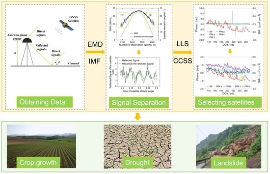
3.1. GNSS Satellite Reflected Signal

SNR is a measurement parameter representing the strength quality of a signal received from the receiver antenna, including the direct and the reflected signals [39,58,59]. At any time, the SNR is a function of direct power, reflected power, and the phase difference between them. Changes in SM will change the phase of the reflected signal and the soil reflectivity [38,39]. Thus, SNR oscillations can provide information about changes in near-surface SM [41]. The geometric principle is shown in Figure 3. Evidently, there is a definite relationship between SNR and the ground environment. Therefore, SNR could be used to establish a multipath effect assessment model, which was conducive to estimating surface environmental parameters.

According to existing research, under the assumed condition that reflection occurs only once, there is a sine (or cosine) functional relationship between SNR observations and the multipath interference phase [38,39]:

$${\mathrm{S}\mathrm{N}\mathrm{R}}^2=S_{\mathrm{d}}^2+S_{\mathrm{r}}^2+2S_{\mathrm{d}}{S}_{\mathrm{r}}\mathrm{c}\mathrm{o}\mathrm{s}\psi$$

(1)

where $S_{\mathrm{d}}$ is the direct signal, representing the low-frequency trend term of the SNR; $S_{\mathrm{r}}$ is the reflected signal, representing the high-frequency modulation term of the SNR [56]$;\psi$ is the phase difference between the direct and the reflected signals.

Since the SM retrieval of GNSS-IR is only related to the reflected signal, it is necessary to remove the direct signal of SNR in the low satellite elevation range. After that, there is still a sine (or cosine) function relationship of fixed frequency between the reflected signal and $\sin \theta$, and the reflected signal ${\mathrm{S}\mathrm{N}\mathrm{R}}_{\mathrm{r}}$ can be expressed as [38].

$${\mathrm{S}\mathrm{N}\mathrm{R}}_{\mathrm{r}}=A\mathrm{c}\mathrm{o}\mathrm{s}\left(\frac{4\pi h}{\lambda }\sin \theta +\phi \right)$$

(2)

where $\lambda$ represents the carrier frequency; $A$ and $\phi$ are the characteristic parameters of the reflected signal to be solved, i.e., amplitude and phase, which can be used to retrieve the variation of the surface environment around the site [38,39].

3.2. EMD for Separating the Modulation Terms

Based on the previous section, the accurate separation of the SNR modulation terms is crucial to solving the multiple phases. Currently, the modulation and trend terms in SNR are extracted mainly by the low-order polynomial or the wavelet transform [38,41,53]. Although these methods can obtain the modulation terms well, they need some prior knowledge. The low-order polynomial needs to predict the type of signal trend term in advance, and the wavelet transform needs to determine the best wavelet basis and the decomposition level. These requirements lead to the experiment process for signal separation becoming complex and less flexible. Compared with these methods, EMD is a better adaptive analysis method. Since it can decompose the signal directly according to the scale characteristics of the signal itself without prior knowledge, it is very suitable for extracting the characteristics of non-stationary signals [60,61]. Moreover, using EMD in signal decomposition can significantly enhance the stability and accuracy of GNSS-IR retrieval, as demonstrated for tidal levels and vegetation effects [19,54]. Hence, this paper used EMD to decompose the SNR signal of each satellite. The SNR signal can be expressed as:

$$f\left(t\right)=\left[a_1,a_2,\dots ,a_t\right],\left(t=\mathrm{1,2},\dots ,l\right)$$

(3)

where $a$ represents the GNSS satellite, and $t$ and $l$ are the observation epoch and its length, respectively.

The basic idea of EMD is to decompose $f\left(t\right)$ into an $m$ intrinsic modal function (IMF) of different time scales and a residual term. The following two conditions must be met for each IMF. First, the number of extreme value points must be equal to or at most one unit different from the number of crossing zero points in the whole sequence; second, the average values of the envelope formed by the local maximum and the envelope formed by the local minimum must be zero [60]. The decomposition process of $f\left(t\right)$ can be expressed as:

$$f\left(t\right)=\sum _{k=1}^m{IMF}_k\left(t\right)+T_m\left(t\right)$$

(4)

where $T_m$ is the residual term of the sequence; $m$ is the number of IMF components; ${IMF}_k\left(t\right)$ is the intrinsic modal function, which reflects the inherent and intrinsic characteristics of the signal itself.

It can be seen that the $f\left(t\right)$ is decomposed into a limited number of IMF that contain the local feature signals of the original signal. The first IMF component is the highest-frequency component of $f\left(t\right)$. As the order of the IMF increases, the frequency of its corresponding components gradually decreases. Ideally, $T_m\left(t\right)$ is used as the low-frequency trend term of the original signal. In practice, due to the comprehensive influence of the satellite orbit and the surrounding environment of the site, the SNR of different satellites varies greatly in different periods, and the frequency change of direct signals may exceed the frequency range of a single IMF component. If the IMF component of the last layer is directly fixed as a trend term, it will cause a big error. Considering the residual component is set as the last IMF component and the combination from the boundary IMF component (${IMF}_T$) to the last IMF component is used as the trend term of the original signal, it is possible to obtain the high-quality SNR modulation term required for subsequent LLS analysis. Therefore, reasonably determining the ${IMF}_T$ of all IMF components is the key to effectively extracting the trend term and the fluctuation term of SNR. The trend term can be expressed as:

$${\mathrm{S}\mathrm{N}\mathrm{R}}_{\mathrm{d}}\left(t\right)=\sum _{k=T}^m{IMF}_k\left(t\right)$$

(5)

In this paper, an automatic determination criterion for EMD trend terms is proposed. According to the linear regression relationship between the original signal and each IMF component, the IMF with high correlation was merged as the trend term of SNR, and the remaining IMF was merged as the modulation term of SNR. The method proposed is referred to as the IMF discriminant method, and the specific process is as follows. (1) The correlation coefficient ($r_0$) between each IMF component and the original sequence are calculated, and the correlation coefficient threshold ($r_m$) is set; (2) the IMF component corresponding to the first $r_0$ greater than $r_m$ is considered as the ${IMF}_T$. Subsequently, the components from the ${IMF}_T$ to the last IMF are combined as trend terms and deleted, while the components from the first IMF to the ${IMF}_{T-1}$ are combined as modulation terms and retained. For different GNSS satellites, the target component determined by this method also varies across multiple IMF components with the change of SNR rather than being fixed. In other words, this method is based on the characteristics of the data themselves rather than on artificial restrictions or definitions; so, it has high flexibility.

3.3. CCSS Method

For the SNR data of the same satellite, its ascending (S) and descending (J) tracks are considered as independent [24]; so, they were processed independently. The amplitude and phase in Equation (2) can be obtained by LLS fitting the separated modulation term of SNR [62]. Since the phase of a satellite can better characterize SM changes [39], it was used for SM retrieval in this paper. However, the phases of different satellites have different sensitivities to SM, and not all satellite tracks are suitable for SM monitoring [51]. So, the satellite phases needed to be selected. According to previous experiments, it was found that the phases of different satellites that are strongly related to the SM reference values have similar regular variations. Taking 2015 DOY96~256 of P043 as an example, the correlation coefficients were calculated between the phases of each satellite solved during this period and the SM reference values, as shown in Figure 4. It can be seen that satellites with high correlation with the SM reference values, such as PRN07, PRN23, PRN30, etc., also had high correlation with each other.

According to this property, and in order to realize satellite selection adaptively, this paper proposes a cross-correlation satellite selection (CCSS) method independent of the SM reference values. The satellites were selected directly according to the degree of cross-correlation between their phase sequences. Therefore, the effective satellites were selected by calculating the cross-correlation coefficients between different satellite phases and then by reasonably setting the threshold range of the cross-correlation coefficient based on the correlation degree (

Table 2. Cross-correlation threshold range.

Degree of Cross-Correlation	Very Weak Correlation	Weak Correlation	Medium Correlation	Strong Correlation	Very Strong Correlation
correlation coefficient	0~0.2	0.2~0.4	0.4~0.6	0.6~0.8	0.8~1

).

The specific process of CCSS was as follows:

• During the experiment, the satellites with relatively complete phase data (more than 95% of the total data) were selected preliminarily. Because for the multisatellite combination retrieval mode, the selected satellite data needed to meet the requirement of continuous and consistent reflection trajectories within the range of satellite interception elevation, the continuous phase could be generated throughout the annual product day observation period.
• Based on the satellites selected in step ➀, the cross-correlation coefficient ($r_1$) between each satellite phase and other satellite phases was calculated separately. Then, considering the medium correlation as the initial reference condition according to the cross-correlation threshold range in Table 2, the satellites with $r_1$ greater than 0.400 were selected as long as they existed, and the satellites without $r_1$ greater than 0.400 were excluded.

  $$r\left({\phi }_a,{\phi }_b\right)=\frac{Cov\left({\phi }_a,{\phi }_b\right)}{\sqrt{Var\left[{\phi }_a\right]}\sqrt{Var\left[{\phi }_b\right]}}$$

  (6)

  where $a$ and $b$ correspond to different (PRN) numbers of GNSS satellites, $Cov({\phi }_a,{\phi }_b)$ is the covariance corresponding to $a$ and $b$, $Var\left[{\phi }_a\right]$ represents the variance of $a$, and $Var\left[{\phi }_b\right]$ represents the variance of $b$.
• The cross-correlation coefficient ($r_a^i$) and its average value ($\overline{r_a^i}$) for each satellite selected in step ➁ were calculated. Then, the threshold ranges ($r_n^i$) of different gradients were set for the cross-correlation coefficient average, and the satellites with $\overline{r_a^i}$ larger than $r_n^i$ were selected. Among them, the setting of $r_n^i$ started from a value greater than 0.400 and increased at intervals of 0.1 each time. Moreover, in every screening process, it was necessary first to eliminate the satellites with $\overline{r_a^i}$ smaller than $r_n^i$, then continue to calculate $r_a^i$ and $\overline{r_a^i}$ for the remained satellites, and only later compare the updated $\overline{r_a^i}$ with the newly set threshold $r_n^i$. This way, the accurate selection of satellites with different precision was realized:

  $$\overline{r_a^i}=\frac{\sum _{n=1}^{m}r\left({\phi }_a,{\phi }_n\right)}{m}\ge r_n^i$$

  (7)

  where $\sum _{n=1}^{m}r\left({\phi }_a,{\phi }_n\right)$ is the sum of the correlation values between satellite $a$ and other $m$ satellites.
• Based on the satellites selected in step ➂, effective satellites within different $r_n^i$ ranges were obtained. We continued to select and process them, eliminating satellites with duplicate ascending and descending segments. For the same satellite, if there was no ascending segment (S), the phase of the descending segment (J) was used; if there was no descending segment, the phase of the ascending segment was used; if both the ascending and the descending segments existed, the satellite within the higher CCSS threshold range was selected.

3.4. MRER Model

Based on the previous section, the phase set of multiple satellites selected by different cross-correlation threshold ranges ($r_n$) can be expressed as:

$$\left\{\begin{array}{c}{x}_a^0=\left[{\phi }_1,{\phi }_2,\dots ,{\phi }_t\right],\left(t=\mathrm{1,2},\dots ,m\right)\\ x=\left[x_1^0,x_2^0,\dots ,x_a^0\right],\left(a=\mathrm{1,2},\dots ,32\right)\end{array}\right.$$

(8)

where $x_a^0$ and $x$ are the phase set of single satellites and multisatellite combinations, respectively, $m$ represents the phase length of the satellite, and $a$ represents the (PRN) number of GNSS satellites.

The training set samples for building the model were $\left\{(x_i^j,y_i|i=\mathrm{1,2},\dots ,t_1;j=\mathrm{1,2},\dots ,c)\right\}(t_1<m,\mathrm{c}\le 32)$, where $x_i^j$ is the multisatellite phase set as the input samples for modeling, $y_i$ is the corresponding SM set as the output samples for modeling, and $x_s^j(s=t+1,t+2,\dots ,m)$ is the input sample set for the testing model. Then, a multi-linear regression model was established as follows:

$$y_i={\beta }_0+{\beta }_1{x}_i^1+{\beta }_2{x}_i^2+\dots +{\beta }_j{x}_i^j+v_i$$

(9)

where $i$ represents the sample length of the modeling, $j$ represents the number of combined satellites for modeling, ${\beta }_0$, ${\beta }_1$, …, ${\beta }_j$ are the regression coefficients of the model, $v_i$ is the residual, including the constant deviation of the regression function and random noise.

Converting Equation (9) into matrix expression:

$$\mathit{Y}=\left[\begin{array}{c}\begin{array}{c}{y}_1\\ y_2\\ ⋮\end{array}\\ y_i\end{array}\right],\mathit{X}=\left[\begin{array}{c}\begin{array}{ccc}1& \cdots & x_i^1\\ 1& \cdots & x_i^2\\ ⋮& ⋮& ⋮\end{array}\\ \begin{array}{ccc}1& \cdots & x_i^j\end{array}\end{array}\right],\mathit{\beta }=\left[\begin{array}{c}\begin{array}{c}{\beta }_0\\ {\beta }_1\\ ⋮\end{array}\\ {\beta }_j\end{array}\right],\mathit{V}=\left[\begin{array}{c}\begin{array}{c}{v}_1\\ v_2\\ ⋮\end{array}\\ v_i\end{array}\right]$$

(10)

where $Y$ and $X$ represent the SM matrices and the phase matrices, respectively; $\mathit{\beta }$ represents the coefficient matrices that need to be solved; $\mathit{V}$ is the residual matrices.

Therefore, the regression model can be expressed as:

$$\mathit{Y}=\mathit{X}\mathit{\beta }+\mathit{V}$$

(11)

A robust estimation can suppress the impact of abnormal values to a certain extent, thus enhancing the number or the quality of the satellites that can be used to monitor SM [63]. In this study, the M estimation was used to replace the traditional least squares estimation. Its basic principle is to use the iterative reweighted least squares (IRLS) method to estimate the regression coefficients [64]. The M estimation criterion can be expressed as:

$$\sum _{i=1}^j{\overline{\mathit{P}}}_{ij}\rho \left(v_i\right)=\sum _{i=1}^j{\overline{\mathit{P}}}_{ij}\rho \left(x_i\widehat{{\beta }_j}-y_i\right)=min$$

(12)

where ${\overline{P}}_{ij}$ represents the robust weight function, the selection of which is the key to a robust estimation. In this paper, the IGGⅢ weight function with “three-stage” estimation was adopted, which has strong robustness and can use information more effectively [65,66].

Subsequently, according to the IRLS principle, the iterative equation of the robust regression could be obtained as follows:

$${\mathit{\beta }}_{\mathbf{I}\mathbf{R}\mathbf{L}\mathbf{S}}={\left({\mathit{X}}^T{\overline{\mathit{P}}}_{ij}\mathit{X}\right)}^{-1}\mathit{X}{\overline{\mathit{P}}}_{ij}\mathit{Y}$$

(13)

It can be seen that the main idea of a robust regression model is to assign different weights to different points according to residuals. Then, the weighting algorithm is iterated several times to optimize the weight ${\beta }_{\mathrm{I}\mathrm{R}\mathrm{L}\mathrm{S}}$. Therefore, the obtained SM has a certain robustness.

4. GNSS-IR SM Retrieval

Based on the methods and principles introduced above, a GNSS-IR SM retrieval model was developed in this paper. Figure 5 shows the overall strategy for the parameter and model determination for SM retrieval using GNSS data. Among the steps, to verify the feasibility and effectiveness of the method, the statistical indicators for the model test results and the SM reference values, including the correlation coefficient (r), the root-mean-square error (RMSE, unit cm³ cm⁻³), the mean absolute error (MAE, unit cm³ cm⁻³), and the maximum error (Max, unit cm³ cm⁻³), were used to analyze and assess the model test results from different combination schemes.

5. Results and Discussion

5.1. Separation of the Modulation Terms

According to the previous description of SNR separation, EMD was used to decompose the SNR of each satellite adaptively, and the decomposition results of PRN 14 and 32 are shown in Figure 6. It can be seen that as the decomposition layers increased, the components from IMF1 to the residual tended to smooth, the frequency decreased in order, and the changing trend among the low-frequency components showed a basic consistent feature. The components of PRN 14 and 32 were further analyzed for correlation with SNR, as shown in

Table 3. Correlation coefficient (r) of each IMF with the original SNR.

IMF	r
	PRN14	PRN32
SNR	1	1
IMF1	0.064	0.015
IMF2	0.065	0.050
IMF3	0.013	0.053
IMF4	0.174	0.051
IMF5	0.018	0.056
IMF6	0.703	0.208
IMF7	0.989	0.925
IMF8	0.989	0.989
IMF9	0.989	0.989
residual	0.905	0.988

. Visibly, the correlation coefficients (r) from IMF1 to the residual gradually increased, and there were obvious cut-off points, such as IMF6 for PRN14 and IMF7 for PRN32. Further, r between IMF1~IMF6 for PRN14 and IMF1~IMF5 for PRN32, which tended to be the high-frequency modulation terms, was less than 0.600. In addition, r between IMF7~residual for PRN14 and IMF6~residual for PRN32, which tended to be the low-frequency trend terms, was greater than 0.600. It follows that the cut-off points for the high- and low-frequency components were not fixed. If one or several layers of IMF were fixed directly as the trend term, this would probably cause large errors. As such, reasonably and flexibly determining the correlation coefficient threshold ($r_m$) corresponding to ${IMF}_T$ was extremely important for effectively separating the modulation and the trend terms of SNR. After many experiments and comparative analyses, it was found that when $r_m$ was 0.600, the decomposition effect was better. Accordingly, $r_m$ was set to 0.600 in this paper. To further compare and analyze the effect of the trend items obtained from the combination of different low-frequency components, the components determined by residual, IMF9~residual, IMF8~residual, IMF7~residual, and the IMF discriminant method were used, and the trend items obtained are shown in Figure 7.

It can be seen in Figure 7 that the trend terms separated by the IMF discriminant method were consistent with the total trend of SNR. By comparison, the fitting results from other single-layer or multi-layer IMF component combinations showed some bias. Therefore, the IMF discriminant method could effectively determine the cut-off points of the trend term and modulation term. The separation results of the modulation and trend terms for different satellites obtained by combining EMD and the IMF determination method are shown in

Table 4. Separation results for the trend and modulation terms from each satellite (DOY98).

Satellite Number	Number of Decomposition Layers of EMD	Number of Layers of Combined Modulation Term	Number of Layers of Combined Trend Term
PRN 01	10	IMF1–4	IMF5–10
PRN 02	10	IMF1–8	IMF9–10
PRN 03	10	IMF1–8	IMF9–10
PRN 04	10	IMF1–8	IMF9–10
PRN 05	10	IMF1–9	IMF10
PRN 06	10	IMF1–8	IMF9–10
PRN 07	10	IMF1–9	IMF10
PRN 09	10	IMF1–6	IMF7–10
PRN 10	10	IMF1–7	IMF8–10
PRN 11	9	IMF1–6	IMF7–10
PRN 12	10	IMF1–7	IMF8–10
PRN 13	10	IMF1–7	IMF8–10
PRN 14	10	IMF1–6	IMF7–10
PRN 15	10	IMF1–8	IMF9–10
PRN 16	10	IMF1–6	IMF7–10
PRN 18	10	IMF1–8	IMF9–10
PRN 19	9	IMF1–8	IMF9–10
PRN 20	10	IMF1–5	IMF6–10
PRN 21	10	IMF1–8	IMF9–10
PRN 22	10	IMF1–8	IMF9–10
PRN 23	10	IMF1–8	IMF9–10
PRN 24	10	IMF1–6	IMF7–10
PRN 25	10	IMF1–8	IMF9–10
PRN 27	10	IMF1–7	IMF8–10
PRN 28	10	IMF1–6	IMF7–10
PRN 29	10	IMF1–8	IMF9–10
PRN 30	9	IMF1–8	IMF9
PRN 32	10	IMF1–6	IMF7–10

. For SNR of different satellites, the number of EMD decomposition layers was basically located in 9~10 layers, and the demarcation points of the trend and modulation term were mainly concentrated in IMF6~IMF8. Therefore, the IMF modulation term components extracted from the SNR of different satellites were not fixed, and the trend term could be accurately separated using the combination of multiple low-frequency IMF components determined by the IMF discrimination method.

5.2. Selection of Available Satellites

Based on combining EMD and the IMF determination method to separate the modulation terms of each satellite, the original phase of each satellite was determined by the LLS fitting. Following the steps in satellite selection, satellites with continuous phases were preliminarily selected, with 17 satellites in both the ascending and the descending segments. The statistics of these satellites relative to the threshold ranges ($r_n$) of different cross-correlation coefficients are shown in

Table 5. Satellite statistics for different threshold ranges of the cross-correlation coefficient ($r_n$ ).

Satellite Number	(S/J)	${\mathit{r}}_{\mathit{n}}$	Satellite Number	(S/J)	${\mathit{r}}_{\mathit{n}}$
PRN 04	S	<0.4	PRN 01	J	<0.4
PRN 09	S	<0.4	PRN 03	J	<0.4
PRN 11	S	<0.4	PRN 11	J	<0.4
PRN 13	S	<0.4	PRN 16	J	<0.4
PRN 27	S	<0.4	PRN 22	J	<0.4
PRN 31	S	<0.4	PRN 23	J	<0.4
PRN 22	S	<0.4	PRN 27	J	<0.4
PRN 03	S	<0.4	PRN 18	J	<0.4
PRN 32	S	0.4–0.5	PRN 21	J	<0.4
PRN 19	S	0.4–0.5	PRN 24	J	<0.4
PRN 24	S	0.5–0.6	PRN 31	J	<0.4
PRN 01	S	0.5–0.6	PRN 15	J	<0.4
PRN 16	S	0.5–0.6	PRN 13	J	0.5–0.6
PRN 14	S	0.6–0.7/0.7–0.8	PRN 32	J	0.5–0.6
PRN 30	S	0.6–0.7/0.7–0.8	PRN 09	J	0.6–0.7
PRN 23	S	0.6–0.7/0.7–0.8	PRN 04	J	0.6–0.7
PRN 07	S	0.6–0.7/0.7–0.8	PRN 14	J	0.7–0.8

S and J in the table represent the ascending and the descending segments of the satellites’ track, respectively.

. It can be seen that there were 14 satellites having lifting tracks with $r_n$ greater than 0.400. Among them, seven satellites had $r_n$ greater than 0.600; they were PRN 14 (S), PRN 30 (S), PRN 23 (S), PRN 07 (S), PRN 09 (J), PRN04 (J), and PRN 14 (J). In addition, the statistical correlation (r) between the phases of the 17 satellites that were in the elevation segment and SM is shown in Figure 8. It can be observed that for the satellites with $\overline{r_a}$ less than 0.400, their corresponding r were below 0.550, which means that the correlations were low or non-existent. Thus, these satellites could not be used for SM retrieval and needed to be eliminated. For the satellites with $\overline{r_a}$ greater than 0.400, their corresponding r were greater than 0.600, implying that these satellites had a strong correlation relevant to SM and could be selected for SM retrieval. Among them, when $r_n$ was above the threshold of 0.700, the correlations of the selected satellites were all greater than 0.750.

To further verify the dispersion degree of the phases from the selected satellites in different $r_n$ ranges, the satellites with repeated ascending and descending segments were eliminated. Then, 12 satellites were left to be analyzed, as shown in Figure 9. It can be seen that when the range of $r_n$ was set lower, some of the selected satellites, such as PRN19, PRN24, PRN01, and PRN16, had poor quality and showed more outliers. As the range of $r_n$ increased, the selected satellites acquired a better observation quality. When the value of $r_n$ was greater than 0.700, the phases of the selected satellites basically showed no abnormal values. To this end, the satellite phases selected by CCSS were used to retrieve SM; schemes are formulated in the next section.

5.3. Retrieval of SM

After completing the selection of the satellite phases, the MRER model entered the processing stage. Following the results in the previous section, 12 satellites were selected for the experiment: PRN 19, PRN 24, PRN 01, PRN 16, PRN 30, PRN 23, PRN 07, PRN 13, PRN 32, PRN 09, PRN 04, and PRN 14. In this experiment, two methods were used to build the MRER model: method 1, i.e., a single-satellite model, and method 2, i.e., a multi-satellite combination model according to the gradually increasing threshold range of $r_n$. For method 1, the MRER model was built directly using a single satellite, and the model test results from 12 satellites were calculated and are shown in scheme 1. Method 2 combined the satellites corresponding to the different ranges of $r_n$; the specific scheme settings are shown in

Table 6. Modeling scheme for the multisatellite combination of method 2.

Scheme	${\mathit{r}}_{\mathit{n}}$	Method 2
2	>0.4	PRN 19, 24, 01, 16, 30, 23, 07,13, 32, 09, 04, 14
3	>0.5	PRN 24, 01, 16, 30, 23, 07, 13, 32, 09, 04, 14
4	>0.6	PRN 30, 23, 07, 09, 04, 14
5	>0.7	PRN 30, 23, 07, 14

. After completing the modeling training, the testing set was input into the model to retrieve SM. The retrieval errors of SM for the different methods are shown in Figure 10.

In Figure 10, it can be seen that whatever the modeling or the testing stages, accurately grasping the variation trend of SM when using a single satellite was difficult, and the retrieval error fluctuated obviously. Especially, for satellites with $r_n$ less than 0.600, such as PRN16 and PRN32, the retrieval effect was poor, and the retrieval process was highly prone to abnormal jumps. It can also be seen from Figure 10 that the retrieval errors of schemes 2 to 5 generally tended to be stable, and the errors mainly fluctuated within the range of −0.070~0.100. Compared with scheme 1, the model was significantly improved. For example, as the cross-correlation coefficients of schemes 4 and 5 were greater than 0.600, the number of combined satellites was reduced. However, the retrieval errors of the models still tended to be stable, but the errors fluctuated less. Additionally, as shown in Figure 2 and Figure 10, the retrieval error of a single satellite gradually increased during the period of continuous precipitation. Especially for the periods of sudden precipitation, such as DOY98~DOY99, DOY116, DOY161~DOY162, and DOY249, the retrieval error values suddenly increased, which might be due to the existence of a certain delay in the SM of single-satellite retrieval. In comparison, the retrieval errors of multisatellite combinations tended to be smooth and basically undisturbed by a sudden or persistent precipitation.

To further assess the performance of each scheme, r, RMSE, MAE, and Max were used, as shown in Figure 11. It can be seen that in the single-satellite scheme, r of the model was low, with a Max generally greater than 0.131, and the ranges of RMSE and MAE were 0.057~0.167 and 0.062~0.155, respectively. In Figure 11, it can also be seen that the modeling results of the multisatellite combination were better, with r greater than 0.918, i.e., 40~44% better than that of a single satellite. RMSE and MAE were less than 0.039, and Max was less than 0.077. It is not difficult to see that the multisatellite robust regression model could effectively restrain the influence of outliers and improve the SM retrieval accuracy. Further comparing scheme 2 to scheme 5, it is surprising that with the gradual improvement of the set range of $r_n$, the changes of r, RMSE, MAE, and Max were still small, although the number of satellite combinations used for modeling decreased. This may be related to both the number and the quality of the selected satellites. When the observation quality of the satellites used for modeling is good, a small number of combined satellites can achieve a higher modeling effect. Therefore, it is worth noting that when the selected satellites had $r_n$ greater than 0.700, the observation quality of these satellites was generally good, and this value could be directly chosen to build multisatellite robust regression models. In this case, only few satellites would be required to improve the results; so, the complexity of modeling is decreased. When each satellite had an $r_n$ of less than 0.600, the observation quality of the satellite was poor; so, combining more satellites would also be a good option.

6. Conclusions

By combining EMD and the IMF discriminant method, the modulation and trend terms of the SNR from different satellites were effectively separated. Compared with the traditional low-order polynomial and wavelet analysis, EMD does not require prior knowledge, so it can directly and adaptively decompose the information of different frequencies implied in the SNR data. It was also found that for the SNR of different satellites, the number of layers obtained by EMD decomposition was inconsistent, and the layers were mainly 9~10. Obviously, when separating the trend and the modulation terms, the high number of many decomposition layers increased the difficulties. To solve this problem, the IMF discriminant method was further used to analyze the correlation between low-frequency and high-frequency components. It could effectively determine the cut-off points of the trend terms and modulation terms for each satellite. When the correlation coefficient threshold $r_m$ corresponding to ${IMF}_T$ was 0.600, the modulation term of each satellite could be accurately extracted. Thus, for the modulation term separation, the combination of EMD and the IMF discrimination method showed stronger self-adaptability and, thus, has more advantages than the low-order polynomial and wavelet transform.

Due to the comprehensive influence of different surface environments and satellite tracks, the response modes of different satellite phases to surface SM changes are inconsistent. The available selection of satellites is the key to the accurate retrieval of SM. The results showed that CCSS could effectively select the available satellites and classify the SNR quality of each satellite to different accuracy levels. Moreover, it reduced the dependence on the SM reference value and achieved an adaptive selection of the satellites. For SM retrieval, the MSER model can fully combine the surface SM information from satellites in different directions, and the model training or the test error is relatively stable. Compared with the single-satellite model, the retrieval accuracy of the multisatellite combination model was effectively enhanced, and the retrieval error of SM in sudden precipitation periods was effectively improved. When the cross-correlation coefficient threshold ($r_n$) of CCSS was set to 0.700 or above, the correlation between the selected satellite phases and the SM reference values was greater than 0.750. Moreover, these selected satellites also achieved better results after being modeled by MSER, with r reaching 0.918, which is a value more than 40% higher than that for the single-satellite model. this fully shows that the satellites selected by using CCSS were effective. Therefore, to reduce the modeling complexity, the range of $r_n$ can be set to 0.700, as the cut-off value to select the satellites. Of course, this conclusion is limited to the observation environment selected in this paper. In addition, if higher precision SM retrieval results are required, it is better to combine all satellites with $r_n$ greater than 0.400.

In the future, this method will be extended to the application of different satellite navigation systems for different vegetation environments. In this process, the problems of vegetation noise removal and satellite selection for multisatellite and multi-frequency combinations need to be further discussed.

References

1. Bastiaanssen, W.; Molden, D.J.; Makin, I.W. Remote sensing for irrigated agriculture: Examples from research and possible applications. Agric. Water Manag. 2000, 46, 137–155. [Google Scholar] [CrossRef]
2. Xu, Y.; Dong, K.; Jiang, M.; Liu, Y.; He, L.; Wang, J.; Zhao, N.; Gao, Y. Soil moisture and species richness interactively affect multiple ecosystem functions in a microcosm experiment of simulated shrub encroached grasslands. Sci. Total Environ. 2022, 803, 149950. [Google Scholar] [CrossRef] [PubMed]
3. Saadatabadi, A.R.; Izadi, N.; Karakani, E.G.; Fattahi, E.; Shamsipour, A.A. Investigating relationship between soil moisture, hydro-climatic parameters, vegetation, and climate change impacts in a semi-arid basin in Iran. Arab. J. Geosci. 2021, 14, 1796. [Google Scholar] [CrossRef]
4. Mohanty, B.P.; Cosh, M.; Lakshmi, V.; Montzka, C. Remote sensing for vadose zone hydrology—A synthesis from the vantage point. Vadose Zone J. 2013, 12, 128. [Google Scholar] [CrossRef] [Green Version]
5. Brocca, L.; Ciabatta, L.; Massari, C.; Camici, S.; Tarpanelli, A. Soil moisture for hydrological applications: Open questions and new opportunities. Water 2017, 9, 140. [Google Scholar] [CrossRef]
6. Ochsner, T.E.; Cosh, M.H.; Cuenca, R.H.; Dorigo, W.A.; Draper, C.S.; Hagimoto, Y.; Kerr, Y.H.; Larson, K.M.; Njoku, E.G.; Small, E.E.; et al. State of the art in large-scale soil moisture monitoring. Soil Sci. Soc. Am. J. 2013, 77, 1888–1919. [Google Scholar] [CrossRef] [Green Version]
7. Xu, L.; Chen, N.; Zhang, X.; Moradkhani, H.; Zhang, C.; Hu, C. In-situ and triple-collocation based evaluations of eight global root zone soil moisture products. Remote Sens. Environ. 2021, 254, 112248. [Google Scholar] [CrossRef]
8. Barre, H.M.; Duesmann, B.; Kerr, Y.H. SMOS: The mission and the system. IEEE Trans. Geosci. Remote Sens. 2008, 46, 587–593. [Google Scholar] [CrossRef]
9. Entekhabi, D.; Njoku, E.G.; Oneill, P.; Spencer, M.; Jackson, T.; Entin, J.; Im, E.; Kellogg, K. The soil moisture active passive mission (SMAP). In Proceedings of the IGARSS 2008–2008 IEEE International Geoscience and Remote Sensing Symposium, Boston, MA, USA, 7–11 July 2008; Volume 3, pp. 1–4. [Google Scholar] [CrossRef]
10. Burgin, M.S.; Colliander, A.; Njoku, E.G.; Chan, S.K.; Cabot, F.; Kerr, Y.H.; Bindlish, R.; Jackson, T.J.; Entekhabi, D.; Yueh, S.H. A comparative study of the smap passive soil moisture product with existing satellite-based soil moisture products. IEEE Trans. Geosci. Remote Sens. 2017, 55, 2959–2971. [Google Scholar] [CrossRef]
11. Xu, H.; Yuan, Q.; Li, T.; Shen, H.; Zhang, L.; Jiang, H. Quality improvement of satellite soil moisture products by fusing with in-situ measurements and GNSS-R estimates in the Western Continental US. Remote Sens. 2018, 10, 1351. [Google Scholar] [CrossRef] [Green Version]
12. Hein, G.W. Status, perspectives and trends of satellite navigation. Satell. Navig. 2020, 1, 22. [Google Scholar] [CrossRef]
13. Jin, S.; Cardellach, E.; Xie, F. GNSS Remote Sensing, Theory, Methods and Applications; Springer: Amsterdam, The Netherlands, 2014; Volume 19, pp. 241–249. [Google Scholar] [CrossRef]
14. Nievinski, F.G.; Larson, K.M. Forward modeling of GPS multipath for near-surface reflectometry and positioning applications. GPS Solute. 2014, 18, 309–322. [Google Scholar] [CrossRef]
15. Wu, X.; Jin, S.; Chang, L. Monitoring Bare Soil Freeze-Thaw Process Using GPS-Interferometric Reflectometry: Simulation and Validation. Remote Sens. 2018, 10, 14. [Google Scholar] [CrossRef] [Green Version]
16. Chew, C.C.; Small, E.E. Soil Moisture Sensing Using Spaceborne GNSS Reflections: Comparison of CYGNSS Reflectivity to SMAP Soil Moisture. Geophys. Res. Lett. 2018, 45, 4049–4057. [Google Scholar] [CrossRef] [Green Version]
17. Munoz-Martin, J.F.; Llaveria, D.; Herbert, C.; Pablos, M.; Park, H.; Camps, A. Soil moisture estimation synergy using gnss-r and l-band microwave radiometry data from fsscat/fmpl-2. Remote Sens. 2021, 13, 994. [Google Scholar] [CrossRef]
18. Nievinski, F.G.; Hobiger, T.; Haas, R.; Liu, W.; Strandberg, J.; Tabibi, S.; Vey, S.; Wickert, J.; Williams, S. SNR-based GNSS reflectometry for coastal sea-level altimetry: Results from the first IAG inter-comparison campaign. J. Geod. 2020, 94, 70. [Google Scholar] [CrossRef]
19. Zhang, S.; Liu, K.; Liu, Q.; Zhang, C.; Zhang, Q.; Nan, Y. Tide variation monitoring based improved GNSS-MR by empirical mode decomposition. Adv. Space Res. 2019, 63, 3333–3345. [Google Scholar] [CrossRef]
20. Larson, K.M.; Nievinski, F.G. GPS snow sensing: Results from the earthscope plate boundary observatory. GPS Solut. 2013, 17, 41–52. [Google Scholar] [CrossRef]
21. Li, Y.; Chang, X.; Yu, K.; Wang, S.; Li, J. Estimation of snow depth using pseudorange and carrier phase observations of GNSS single-frequency signal. GPS Solut. 2019, 23, 118. [Google Scholar] [CrossRef]
22. Lei, J.; Li, W.; Zhang, S. Improving Consistency of GNSS-IR Reflector Height Estimates between Different Frequencies Using Multichannel Singular Spectrum Analysis. Remote Sens. 2023, 15, 1779. [Google Scholar] [CrossRef]
23. Su, M.; Zheng, F.; Shang, J.; Qiao, L.; Qiu, Z.; Zhang, H.; Zheng, J. Influence of flooding on GPS carrier-to-noise ratio and water content variation analysis: A case study in Zhengzhou, China. GPS Solut. 2023, 27, 21. [Google Scholar] [CrossRef]
24. Wan, W.; Larson, K.M.; Small, E.E.; Chew, C.C.; Braun, J.J. Using geodetic GPS receivers to measure vegetation water content. GPS Solut. 2015, 19, 237–248. [Google Scholar] [CrossRef]
25. Camps, A.; Alonso-Arroyo, A.; Park, H.; Onrubia, R.; Pascual, D.; Querol, J. L-band vegetation optical depth estimation using transmitted gnss signals: Application to gnss-reflectometry and positioning. Remote Sens. 2020, 12, 2352. [Google Scholar] [CrossRef]
26. Martin-Neira, M. A passive reflectometry and interferometry system (PARIS): Application to ocean altimetry. ESA J. 1993, 17, 331–355. [Google Scholar]
27. Lowe, S.T.; Zuffada, C.; Chao, Y.; Kroger, P.; Young, L.E.; LaBrecque, J.L. 5-cm-Precision aircraft ocean altimetry using GPS reflections. Geophys. Res. Lett. 2002, 29, 13-1–13-4. [Google Scholar] [CrossRef] [Green Version]
28. Li, W.; Yang, D.; D’Addio, S.; Martín-Neira, M. Partial Interferometric Processing of Reflected GNSS Signals for Ocean Altimetry. IEEE Geosci. Remote Sens. Lett. 2014, 11, 1509–1513. [Google Scholar] [CrossRef]
29. Clarizia, M.P.; Ruf, C.; Cipollini, P.; Zuffada, C. First spaceborne observation of sea surface height using GPS-reflectometry. Geophys. Res. Lett. 2016, 43, 767–774. [Google Scholar] [CrossRef] [Green Version]
30. Ban, W.; Yu, K.; Zhang, X. GEO-satellite-based reflectometry for soil moisture estimation: Signal modeling and algorithm development. IEEE Trans. Geosci. Remote Sens. 2018, 56, 1829–1838. [Google Scholar] [CrossRef]
31. Calabia, A.; Molina, I.; Jin, S. Soil moisture content from GNSS reflectometry using dielectric permittivity from Fresnel reflection coefficients. Remote Sens. 2020, 12, 122. [Google Scholar] [CrossRef] [Green Version]
32. Yan, Q.; Huang, W.; Jin, S.; Jia, Y. Pan-tropical soil moisture mapping based on a three-layer model from CYGNSS GNSS-R data. Remote Sens. Environ. 2020, 247, 111944. [Google Scholar] [CrossRef]
33. Munoz-Martin, J.F.; Rodriguez-Alvarez, N.; Bosch-Lluis, X.; Oudrhiri, K. Analysis of polarimetric GNSS-R Stokes parameters of the Earth’s land surface. Remote Sens. Environ. 2023, 287, 113491. [Google Scholar] [CrossRef]
34. Yu, K.; Li, Y.; Jin, T.; Chang, X.; Wang, Q.; Li, J. GNSS-R-based snow water equivalent estimation with empirical modeling and enhanced SNR-based snow depth estimation. Remote Sens. 2020, 12, 3905. [Google Scholar] [CrossRef]
35. Hu, Y.; Yuan, X.; Liu, W.; Hu, Q.; Wickert, J.; Jiang, Z. An SVM-based snow detection algorithm for GNSS-R snow depth retrievals. IEEE J. Sel. Top. Appl. Earth Obs. Remote Sens. 2022, 15, 6046–6052. [Google Scholar] [CrossRef]
36. Guo, W.; Du, H.; Guo, C.; Southwell, B.J.; Cheong, J.W.; Dempster, A.G. Information fusion for GNSS-R wind speed retrieval using statistically modified convolutional neural network. Remote Sens. Environ. 2022, 272, 112934. [Google Scholar] [CrossRef]
37. Rodriguez-Alvarez, N.; Bosch-Lluis, X.; Camps, A.; Vall-Llossera, M.; Valencia, E.; Marchan-Hernandez, J.F.; Ramos-Perez, I. Soil moisture retrieval using GNSS-R techniques: Experimental results over a bare soil field. IEEE Trans Geosci. Remote Sens. 2009, 47, 3616–3624. [Google Scholar] [CrossRef]
38. Larson, K.M.; Small, E.E.; Gutmann, E.; Bilich, A.; Axelrad, P.; Braun, J. Using GPS multipath to measure soil moisture fluctuations: Initial results. GPS Solut. 2008, 12, 173–177. [Google Scholar] [CrossRef]
39. Chew, C.C.; Small, E.E.; Larson, K.M.; Zavorotny, V.U. Effects of Near-Surface Soil Moisture on GPS SNR Data: Development of a Retrieval Algorithm for Soil Moisture. IEEE Trans. Geosci. Remote Sens. 2014, 52, 537–543. [Google Scholar] [CrossRef]
40. Roussel, N.; Frappart, F.; Ramillien, G.; Darrozes, J.; Baup, F.; Lestarquit, L.; Ha, M.C. Detection of Soil Moisture Variations Using GPS and GLONASS SNR Data for Elevation Angles Ranging From 2 degrees to 70 degrees. IEEE J. Sel. Top. Appl. Earth Obs. Remote Sens. 2016, 9, 4781–4794. [Google Scholar] [CrossRef]
41. Chew, C.C.; Small, E.E.; Larson, K.M. An algorithm for soil moisture estimation using GPS-interferometric reflectometry for bare and vegetated soil. GPS Solut. 2016, 20, 525–537. [Google Scholar] [CrossRef]
42. Small, E.E.; Larson, K.M.; Chew, C.; Dong, J.; Ochsner, T.E. Validation of GPS-IR soil moisture retrievals: Comparison of different algorithms to remove vegetation effects. IEEE J. Sel. Top. Appl. Earth Obs. Remote Sens. 2016, 9, 4759–4770. [Google Scholar] [CrossRef]
43. Zhang, S.; Calvet, J.C.; Darrozes, J.; Roussel, N.; Frappart, F.; Bouhours, G. Deriving surface soil moisture from reflected GNSS signal observations from a grassland site in southwestern France. Hydrol. Earth Syst. Sci. 2018, 22, 1931–1946. [Google Scholar] [CrossRef] [Green Version]
44. Lv, J.; Zhang, R.; Tu, J.; Liao, M.; Pang, J.; Yu, B.; Li, K.; Xiang, W.; Fu, Y.; Liu, G. A GNSS-IR Method for Retrieving Soil Moisture Content from Integrated Multi-Satellite Data That Accounts for the Impact of Vegetation Moisture Content. Remote Sens. 2021, 13, 2442. [Google Scholar] [CrossRef]
45. Ran, Q.; Zhang, B.; Yao, Y.; Yan, X.; Li, J. Editing arcs to improve the capacity of GNSS-IR for soil moisture retrieval in undulating terrains. GPS Solut. 2022, 26, 19. [Google Scholar] [CrossRef]
46. Tabibi, S.; Nievinski, F.G.; van Dam, T.; Monico, J.F. Assessment of modernized GPS L5 SNR for ground-based multipath reflectometry applications. Adv. Space Res. 2015, 55, 1104–1116. [Google Scholar] [CrossRef] [Green Version]
47. Vey, S.; Güntner, A.; Wickert, J.; Blume, T.; Ramatschi, M. Long-term soil moisture dynamics derived from GNSS interferometric reflectometry: A case study for Sutherland, South Africa. GPS Solut. 2016, 20, 641–654. [Google Scholar] [CrossRef]
48. Yang, T.; Wan, W.; Chen, X.; Chu, T.; Qiao, Z.; Liang, H.; Wei, J.; Wang, G.; Hong, Y. Land surface characterization using BeiDou signal-to-noise ratio observations. GPS Solut. 2019, 23, 32. [Google Scholar] [CrossRef]
49. Chen, K.; Cao, X.; Shen, F.; Ge, Y. An Improved Method of Soil Moisture Retrieval Using Multi-Frequency SNR Data. Remote Sens. 2021, 13, 3725. [Google Scholar] [CrossRef]
50. Nie, S.; Wang, Y.; Tu, J.; Li, P.; Xu, J.; Li, N.; Wang, M.; Huang, D.; Song, J. Retrieval of Soil Moisture Content Based on Multisatellite Dual-Frequency Combination Multipath Errors. Remote Sens. 2022, 14, 3193. [Google Scholar] [CrossRef]
51. Liang, Y.; Lai, J.; Ren, C.; Lu, X.; Zhang, Y.; Ding, Q.; Hu, X. GNSS-IR multisatellite combination for soil moisture retrieval based on wavelet analysis considering detection and repair of abnormal phases. Measurement 2022, 203, 111881. [Google Scholar] [CrossRef]
52. Han, M.; Zhu, Y.; Yang, D.; Hong, X.; Song, S. A semi-empirical SNR model for soil moisture retrieval using GNSS SNR data. Remote Sens. 2018, 10, 280. [Google Scholar] [CrossRef] [Green Version]
53. Wang, X.; Zhang, Q.; Zhang, S. Water levels measured with SNR using wavelet decomposition and Lomb-Scargle periodogram. GPS Solut. 2018, 22, 22. [Google Scholar] [CrossRef]
54. Zhang, S.; Wang, T.; Wang, L.; Zhang, J. Evaluation of GNSS-IR for retrieving soil moisture and vegetation growth characteristics in wheat farmland. J. Surv. Eng. 2021, 147, 04021009. [Google Scholar] [CrossRef]
55. Dunn, M.J. Global Positioning Systems Wing (GPSW) Systems Engineering & Integration, Interface Specification IS-GPS-200. 2010; pp. 1–226. Available online: http://www.gps.gov/technical/icwg/IS-GPS-200E.pdf (accessed on 5 May 2023).
56. Zavorotny, V.U.; Larson, K.M.; Braun, J.J.; Small, E.E.; Gutmann, E.D.; Bilich, A.L. A Physical Model for GPS Multipath Caused by Land Reflections: Toward Bare Soil Moisture Retrievals. IEEE J. Sel. Top. Appl. Earth Obs. Remote Sens. 2010, 3, 100–110. [Google Scholar] [CrossRef]
57. Schwarz, G.E.; Alexander, R.B. Soils Data for the Conterminous United States Derived from the NRCS State Soil Geographic (STATSGO) Data Base. US Geological Survey Open-File Report. 1995; pp. 95–449. Available online: https://water.usgs.gov/lookup/getspatial?ussoils (accessed on 5 May 2023).
58. Bilich, A.; Larson, K.M. Correction to “mapping the GPS multipath environment using the signal to noise ratio (SNR)”. Radio Sci. 2008, 43, 3442–3446. [Google Scholar] [CrossRef]
59. Tong, Z.; Su, M.; Zheng, F.; Shang, J.; Wu, J.; Shen, X.; Chang, X. Accurate Retrieval of the Whole Flood Process from Occurrence to Recession Based on GPS Original CNR, Fitted CNR, and Seamless CNR Series. Remote Sens. 2023, 15, 2316. [Google Scholar] [CrossRef]
60. Huang, N.E.; Shen, Z.; Long, S.S.; Wu, M.C.; Shih, H.H.; Zheng, Q.; Yen, N.C.; Tung, C.C.; Liu, H.H. The empirical mode decomposition and the Hilbert spectrum for nonlinear and non-siteary time series analysis. Proc. R. Soc. London. Ser. A Math. Phys. Eng. Sci. 1988, 454, 903–995. [Google Scholar] [CrossRef]
61. Beckheinrich, J.; Hirrle, A.; Schön, S.; Beyerle, G.; Semmling, M.; Wickert, J. Water level monitoring of the Mekong Delta using GNSS reflectometry technique. In Proceedings of the 2014 IEEE Geoscience and Remote Sensing Symposium, Quebec City, QC, Canada, 13–18 July 2014; pp. 3798–3801. [Google Scholar] [CrossRef]
62. Johnson, M.L.; Correia, J.J.; Yphantis, D.A.; HalvorSON, H.R. Analysis of data from the analytical ultracentrifuge by nonlinear least-squares techniques. Biophys. J. 1981, 36, 575–588. [Google Scholar] [CrossRef] [Green Version]
63. Jing, L.; Yang, L.; Yang, W.; Xu, T.; Gao, F.; Lu, Y.; Sun, B.; Yang, D.; Hong, X.; Wang, N.; et al. Robust Kalman Filter Soil Moisture Inversion Model Using GPS SNR Data—A Dual-Band Data Fusion Approach. Remote Sens. 2021, 13, 4013. [Google Scholar] [CrossRef]
64. Huber, P.J.; Ronchetti, E.M. Robust Statistics. In Wiley Series in Probability and Statistics, 2nd ed.; John Wiley & Sons: Hoboken, NJ, USA, 2009. [Google Scholar] [CrossRef]
65. Yang, Y. Robust Estimation for Dependent Observations. Manuscr. Geod. 1994, 19, 10–17. [Google Scholar]
66. Yang, Y.; Song, L.; Xu, T. Robust estimator for correlated observations based on bifactor equivalent weights. J. Geod. 2002, 76, 353–358. [Google Scholar] [CrossRef]
Figure 1. Environment (left panel) and effective observation area (right panel) of P043. The yellow mark indicates the site location of the receiver. The colored ellipse on the ground is the reflection area of each satellite during the research periods when setting an elevation interval between 5°and 20°. These images can be accessed at http://earth.google.com/, accessed on 5 May 2023 and http://www.unavco.org/, accessed on 5 May 2023.
Remotesensing 15 03218 g001
Figure 2. SM reference and precipitation data. Shown are daily averages for the study area, which were obtained from the International Soil Moisture Network (https://ismn.geo.tuwien.ac.at/en/, accessed on 5 May 2023).
Remotesensing 15 03218 g002
Figure 3. Geometric principle illustrating the relationship between multipath signals of SNR and the ground environment. In the figure, h is the vertical distance from the GNSS antenna center to the horizontal ground surface, which is called vertical reflection distance; θ represents the angle between the satellite signal and the slope.
Remotesensing 15 03218 g003
Figure 4. Correlation coefficient of different satellite phases and SM (2015 DOY96~256). In the figure, the color change from dark green to light yellow indicates a change in correlation from 0 to 1. The darker the color, the lower the correlation, and vice versa.
Remotesensing 15 03218 g004
Figure 5. Flowchart for retrieving SM. For the model establishment, the previous 70% of all data from DOY98 to DOY209 were used as the training set, and the following 30% from DOY210 to DOY256 were used as the test set.
Remotesensing 15 03218 g005
Figure 6. The decomposition results of EMD. In the Figure, the horizontal axis represents the epoch of the satellite, and the vertical axis represents the amplitude of the signal. The intrinsic mode function is represented from IMF1 to the residual, with a gradually decreasing frequency. Due to limited space, only the decomposition results for PRN 14 and 32 were randomly selected for display.
Remotesensing 15 03218 g006
Figure 7. The comparison of the SNR trend terms. The fitting results of different IMF combinations of PRN14 and PRN32 are shown. In the Figure, the black line represents the original SNR, and the colored line is the fitted trend term.
Remotesensing 15 03218 g007
Figure 8. Values of r between phases of the initially selected satellites and SM. The ascending (left panel) and descending (right panel) segments are shown.
Remotesensing 15 03218 g008
Figure 9. Linear regression analysis of the phases of the certain initially selected satellites and SM. In the graph, the solid line represents the linear regression trend. The results are shown for a total of 12 satellites, and these satellites were characterized by different cross-correlation threshold ranges.
Remotesensing 15 03218 g009
Figure 10. SM retrieval errors of the different methods. Top and left bottom panels: single-satellite model corresponding to method 1. Right bottom panel: multisatellite combination model corresponding to method 2.
Remotesensing 15 03218 g010
Figure 11. The different assessment results of each method. Top panel: Correlation (r) between the model test results and the SM reference values. Method 1 and method 2 are represented. Bottom panel: RMSE, MAE, and Max of the model testing. Method 1 and method 2 are represented.
Remotesensing 15 03218 g011