Improving Spaceborne GNSS-R Algal Bloom Detection with Meteorological Data

Abstract

Algal bloom has become a serious environmental problem caused by the overgrowth of plankton in many waterbodies, and effective remote sensing methods for monitoring it are urgently needed. Global navigation satellite system-reflectometry (GNSS-R) has been developed rapidly in recent years, which offers a new perspective on algal bloom detection. When algal bloom emerges, the water surface will turn smoother, which can be detected by GNSS-R. In addition, meteorological parameters, such as temperature, wind speed and solar radiation, are generally regarded as the key factors in the formation of algal bloom. In this article, a new algal bloom detection method aided by machine learning and auxiliary meteorological data is established. This work employs the Cyclone GNSS (CYGNSS) data and the fifth generation European Reanalysis (ERA-5) data with the application of the random under sampling boost (RUSBoost) algorithm. Experiments were carried out for Taihu Lake, China, over the period of August 2018 to May 2022. During the evaluation stage, the test true positive rate (TPR) of 81.9%, true negative rate (TNR) of 82.9%, overall accuracy (OA) of 82.9% and the area under (receiver operating characteristic) curve (AUC) of 0.88 were achieved, with all the GNSS-R observables and meteorological factors being involved. Meanwhile, the contribution of each meteorological factor and the error sources were assessed, and the results indicate that temperature and solar radiation play a prominent role among other meteorological factors in this research. This work demonstrates the capability of CYGNSS as an effective tool for algal bloom detection and the inclusion of meteorological data for further enhanced performance.

1. Introduction

With the development of human society, more and more people settle down near inland lakes, which causes the problems of water pollution and consequent water eutrophication [1]. The fertile water is a breeding ground for plankton, and algal bloom will occur under this circumstance [2]. Algal bloom consumes a considerable amount of oxygen and produces toxins in the water, which greatly affects the drinking water safety of the surrounding cities [3,4]. Meanwhile, the frequent emergence of algal bloom will also cause serious damage to the water environment, leading to the massive death of aquatic organisms [5] and undermining the local aquaculture and fishery resources.

To reduce the threats of algal bloom to the lakes and the coastal areas, many monitoring methods have been applied. Traditional field investigations directly measure the concentration of different kinds of algae and the toxins they have produced in the water, but the number and range of the samples are quite limited [6]. The cost of field investigation is also very high, so it is difficult to obtain bloom information about the whole lake and monitor its change in a rapid way. Remote sensing technology has been successfully applied in the field of algal bloom monitoring and research during recent decades; it has the advantages of low expense and ability to observe targets at a large scale [7]. Optical remote sensing data in visible light and infrared band can distinguish the algal bloom-covered area from lake water well for the reason that the reflectance of bloom in different bands differs from that of water, especially in the near-infrared band. Meanwhile, the optical remote sensing method can also be used to perform regression analysis of the algal bloom density. Commonly used spaceborne optical data from the Earth Observing System (EOS), Landsat and Sentinel satellites are suitable for algal bloom observation [6]. However, on cloudy or rainy days, optical sensors cannot obtain sufficiently high-quality data [8], leading to gaps in the observation sequences. Moreover, the temporal resolution of spaceborne optical data is usually not very high, for example, Landsat-8 and Sentinel-2 satellites need at least 8 days to pass the same area again [9].

Monitoring algal bloom in the microwave band has also proved to be effective. Compared with optical sensors, it can observe targets day and night, and in bad weather. Synthetic aperture radar (SAR) is an active microwave remote sensing method that mainly relies on the backscattered radiation of the electromagnetic wave transmitted by itself to detect the scattering surface. Wang et al. [10] showed that the bloom-covered lake surface could suppress radar wave backscattering and result in a ‘dark area’ in SAR images. Although SAR can overcome many of the shortcomings of the optical method, the temporal resolution of most spaceborne SAR data still fails to meet the requirement of daily monitoring [9]. The cost of SAR is relatively high among other remote-sensing instruments, as SAR satellites need to carry the transmitter onboard, and the preprocessing methods for SAR images are also complicated [11]. Airborne optical and SAR remote sensing methods are relatively flexible in observation time and spatial resolution [12], but they are poor in both spatial coverage and platform stability.

Global navigation satellite system-reflectometry (GNSS-R) is an emerging technology in the field of remote sensing. It is an active remote sensing method, which collects the forward reflected L-band signals transmitted by GNSS satellites from the earth’s surface to infer information about the specular point (SP). Similar to other microwave remote sensing methods, GNSS-R can avoid the signal attenuation caused by cloud and dust to a great extent. So far, GNSS-R has been employed in many research domains, for instance, altimetry [13], sea ice detection and thickness measurement [14,15], flood and inland waterbody mapping [11,16,17], sea surface wind retrieving [18,19] and soil moisture inversion [20,21,22].

The remote sensing of algal bloom using GNSS-R has become an interesting topic. Rodriguez-Alvarez et al. [23] proposed using bistatic radar to monitor algal bloom in the Gulf of Mexico for the first time. Ban et al. [24] studied the change of the sea surface roughness and dielectric constant after being covered by the red tide. Zhang et al. [25] firstly analyzed the feasibility of spaceborne GNSS-R algal bloom detection in Taihu Lake, China. They used a GNSS-R observable called the power ratio (PR), with Sentinel-3 OLCI data collected from April to August 2020 as a reference, and discussed the influence of wind speed on the detection accuracy. They regarded PR > 2 as coherent reflection or the existence of bloom, and they found that in the wind speed section of 1–2.5 m/s, the PR-based detection method can achieve the best detection accuracy. Subject to the temporal resolution of Sentinel-3 and the rainy summer climate of Taihu Lake, actually, only 9 days of Sentinel reference data and only 120 preprocessed GNSS-R data points could be obtained. In summary, the results and analyses of the current research are intuitive, and the amount of employed data is insufficient. Additionally, wind speeds of less than 1 m/s are not discussed, making the research results not convincing nor robust enough without comprehensive assessment of the detection results. Although Zhang et al. [25] considered the influencing factor of wind speed, other related meteorological factors, such as wind direction and precipitation, remain to be investigated. Some meteorological factors, such as temperature and solar radiation, do not immediately cause algal bloom. They mainly take effect in the growth stage of plankton, which are also worth studying. To further verify the feasibility of detecting algal bloom with GNSS-R and meteorological data, more observed GNSS-R data and more meteorological factors with time memory should be involved.

The machine learning (ML) method is an effective tool in remote sensing [26,27]. Specifically, it has successfully addressed such problems as classification and regression in remote sensing precisely and effectively. Since the adoption of neural networks for sea ice sensing [28], combining ML with GNSS-R has become a new tendency in recent years. For instance, Zhu et al. [29] applied decision tree (DT) and random forest (RF) in GNSS-R sea ice concentration (SIC) inversion. Ref. [30] employed ML methods in GNSS-R SM retrieval.

In practical research, classification problems may occur such that the data of different labels are imbalanced (‘imbalance’ refers to the disproportionate proportion in the class label). Specifically, the data of one category can be much sparser than those of other types, but the importance of the minority should be emphasized despite its lower proportion. Algal bloom detection via GNSS-R faces such a challenge of an imbalanced dataset. In other words, algal bloom will not take up a great proportion in the whole dataset, but its damage is non-negligible. Traditional classifiers assume that the number of points in each class is generally comparable, and they aim to reach the highest overall accuracy (OA). However, if applying these traditional classifiers to imbalanced datasets, the minority class will be neglected due to its small contribution to the OA, leading to the failure of identifying the minority class. In order to deal with it, the random under sampling (RUS) boosted (RUSBoost) algorithm [31], an algorithm designed for processing imbalanced datasets, can be deployed. RUSBoost is an algorithm that combines RUS with adaptive boosting (AdaBoost, an algorithm that trains many weak classifiters and integrates them into a strong classifier to improve the classification performance; more details are in [32]) and takes advantage of both of them. The RUS algorithm randomly removes samples from the majority class until its number of samples is equal to that of the minority class. RUS can help simplify the algorithm complexity effectively but suffers from a loss of information, while in RUSBoost, with the combination of boosting, the disadvantage of losing information caused by RUS can be well settled. Compared with another commonly used imbalanced data classifier, synthetic minority oversampling technique boosted (SMOTEBoost), RUSBoost saves a great deal of time in training, mostly has better performance, and can better avoid the problem of overfitting.

In view of the shortcomings of the existing research and the challenge of fusing different sources of data, in this paper, we propose a new algal bloom detection method that combines spaceborne GNSS-R data with meteorological factors via the ML method.After necessary preprocessing steps, we screened 2913 GNSS-R points, much more than previous studies with only hundreds of points. Not only was the data amount increased, but also meteorological factors with 10-day time memory before the observation date were added, along with introducing the RUSBoost algorithm for dealing with the imbalanced multi-source data for the first time in the field of spaceborne GNSS-R algal bloom detection. In this way, the interference of wind speed to GNSS-R data was mitigated, and the factors related to the growth mechanism of algal bloom were also considered. Relative to the previous studies, the detection accuracy is progressed significantly in this research. This paper is outlined as follows: Section 2 introduces the research area, datasets of the observed GNSS-R data, auxiliary data of the reanalysis meteorological data and reference optical remote sensing data. In Section 3, the GNSS-R observables and RUSBoost algorithm are described in detail. Section 4 shows the detection results and provides discussion. Section 5 is the conclusion of this research.

2. Datasets

2.1. Area of Interest

Cyanobacteria bloom (a kind of algal bloom) is a commonly seen disaster and has caused serious environment problems in Taihu Lake, China. For this reason, it is chosen as the area of interest (30.9°–31.6°N, 119.9°–120.6°E) of this paper (shown in Figure 1). Taihu Lake is the third largest freshwater lake in China, located in the densely populated Yangtze River Delta. It experiences a subtropical monsoon climate [33]. Taihu Lake became eutrophic in the 1980s. Later in the 1990s, cyanobacteria bloom started to emerge [2]. The average water depth of Taihu Lake is only about 2 m [34]; the shallow water and large amount of lakebed silt also contribute to the growth of cyanobacteria [35,36], as they make the lake water warmer and more fertile. Considering that the eastern part of Taihu Lake is the aquatic plant zone, the growth of cyanobacteria and remote sensing observation here are both influenced, so east of the lake surface to 120.24°E is excluded.

In this work, information about CYGNSS observation data, auxiliary land component of the fifth generation of European Reanalysis (ERA5-Land) data and reference moderate-resolution imaging spectroradiometer (MODIS) data are introduced as follows.

2.2. CYGNSS Data

Cyclone GNSS (CYGNSS) data are widely used GNSS-R data in recent years on account of their high performance in resolution and data quality. CYGNSS satellites were launched at the end of 2016, and the mission was firstly designed for monitoring tropical cyclones over low-latitude ocean (38°S–38°N) by GNSS-R. It is a constellation of eight satellites working in the low earth orbit (LEO) of 510 km, whose revisit period is merely about several hours [37]. Nowadays, applications of CYGNSS data have been expanded to land observation and have received satisfactory results. Apart from the high temporal resolution, the spatial resolution has also progressed a lot relative to previous GNSS-R missions, and its highest spatial resolution is about 0.5 km × 3.5 km [38], which is sufficient for cyanobacteria bloom monitoring. In this research, 2913 data points of CYGNSS Level 1 Version 3.0 product from August 2018 to May 2022 are employed from 212 days, where the reference MODIS data with high quality could be obtained, and they are available at https://podaac-tools.jpl.nasa.gov, accessed on 1 June 2022. Because of the inactive growth of cyanobacteria on cold days, data in winter months (December, January and February) are excluded. Delay-Doppler map (DDM) is the basic observable of GNSS-R; many other observables can be calculated from it to judge the surface condition of SPs. In the CYGNSS dataset, each DDM is saved in 11 Doppler shifts and 17 time delays, containing the reflected signals from SP and the surrounding area. Basic information about every CYGNSS SP is also included in the dataset, for example, its longitude and latitude coordinates, signal incidence angle, and antenna gains. Data points with an incidence angle > 60° and receiver antenna gain < 0 are removed in this study due to their low quality. It needs to be pointed out that only CYGNSS data obtained from 7 a.m. to 7 p.m. on the days where (nearly) cloud-free MODIS images could be accessed are adopted in the research.

2.3. Auxilliary ERA5-Land Data

ERA5-Land data are released by European Centre for Medium range Weather Forecasts (ECMWF) and provide climate reanalysis data from 1950 to the present [39]. They are the latest generation reanalysis data of ECMWF, with their spatial and temporal resolution, model parameterization and data assimilation method being vastly improved relative to other reanalysis products [40], which can be obtained from https://cds.climate.copernicus.eu, accessed on 30 July 2022. The hourly ERA5-Land data are in the grid of 0.1${}^{\circ }\times$ 0.1${}^{\circ }$, with the spatial and temporal coverage being the same as those of the research area. Meteorological factors that can affect the growing and gathering process of cyanobacteria are selected, including wind speed and direction (WS and WD, calculated from dataset ‘10m u/v component of wind’), temperature (T, ‘2m temperature’), total precipitation of one day (ToP, ‘total precipitation’), pressure (P, ‘Surface pressure’) and solar radiation downwards (SRD, ‘surface solar radiation downwards’) during the period of 10 days before the observation date is read and averaged from the ERA5-Land dataset. The averaged ERA5-Land data in this time period will pair up with the selected CYGNSS data points on the observation date. CYGNSS data points and ERA5-Land data rasters are spatially matched based on latitude and longitude coordinates.

2.4. Reference MODIS Data

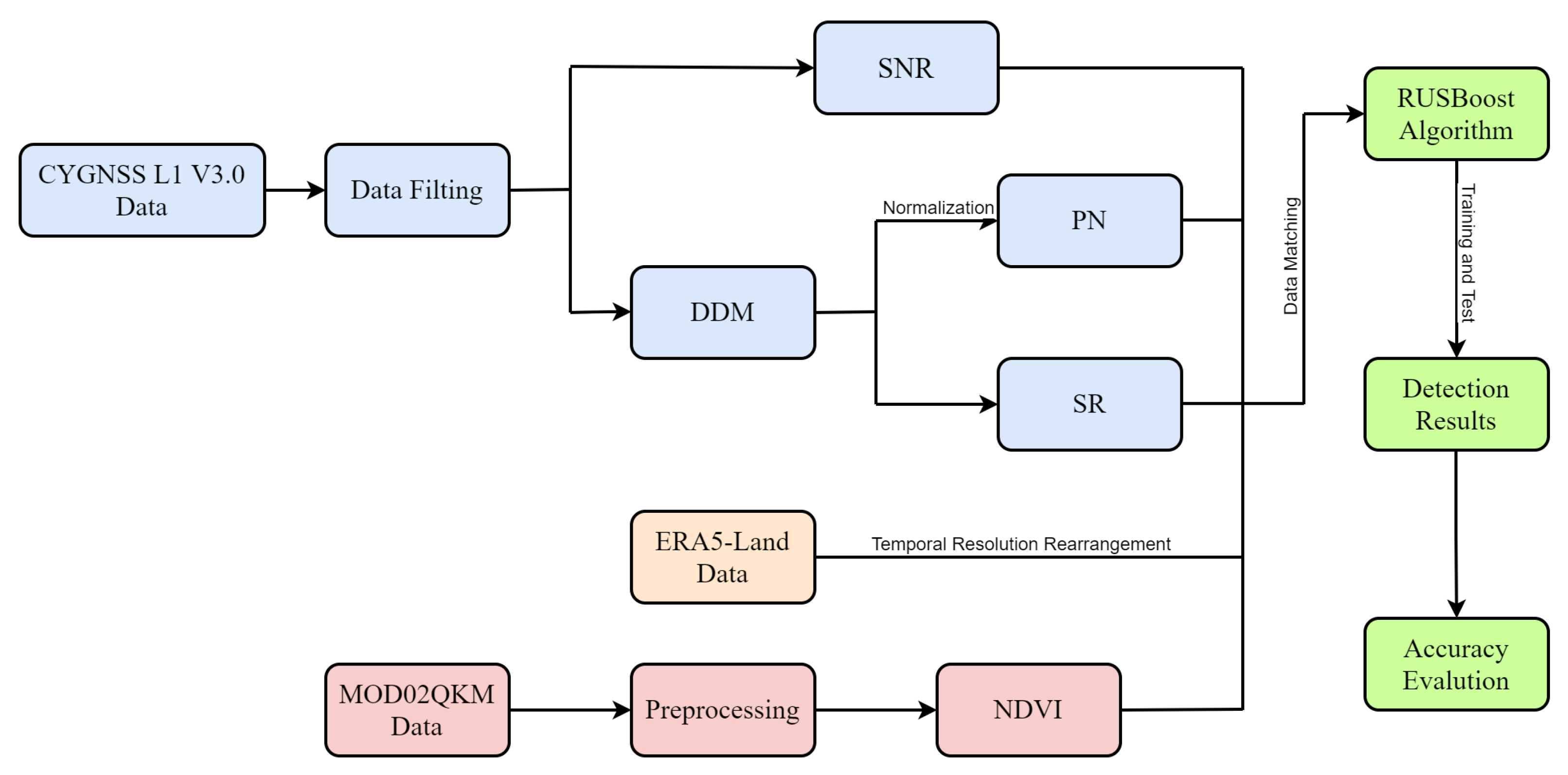
Here, MOD02QKM data (MODIS L1B product, downloaded from https://ladsweb.modaps.eosdis.nasa.gov, accessed on 15 October 2022) are used for calculating the normalized difference vegetation index (NDVI) reference data. The reason for making the reference data by ourselves is that the daily resolution NDVI products in the region of Taihu Lake are not easy to be found. The MODIS L1B product comes with geographic location information and radiometric calibration parameters; in this way, it can be preprocessed directly by the Georeference MODIS tool in ENVI 5.6. Red light band and near-infrared band are contained in MOD02QKM data with the original spatial resolution of 250 m × 250 m and in the daily resolution. Then, calculating the NDVI index by the two bands above is as follows:

$$NDVI=\frac{NIR-R}{NIR+R},$$

(1)

where R refers to the reflectance in the red band and $NIR$ refers to that in the near-infrared band. Pixels with a NDVI value > 0.05 will be regarded as occupied cyanobacteria bloom. When verifying the correctness of detection, if there are more than 15 bloom pixels in the 5 × 5 pixels, the central pixel of which the CYGNSS data point is located, this CYGNSS data point is labeled as a cyanobacteria bloom point.

3. Detection Method

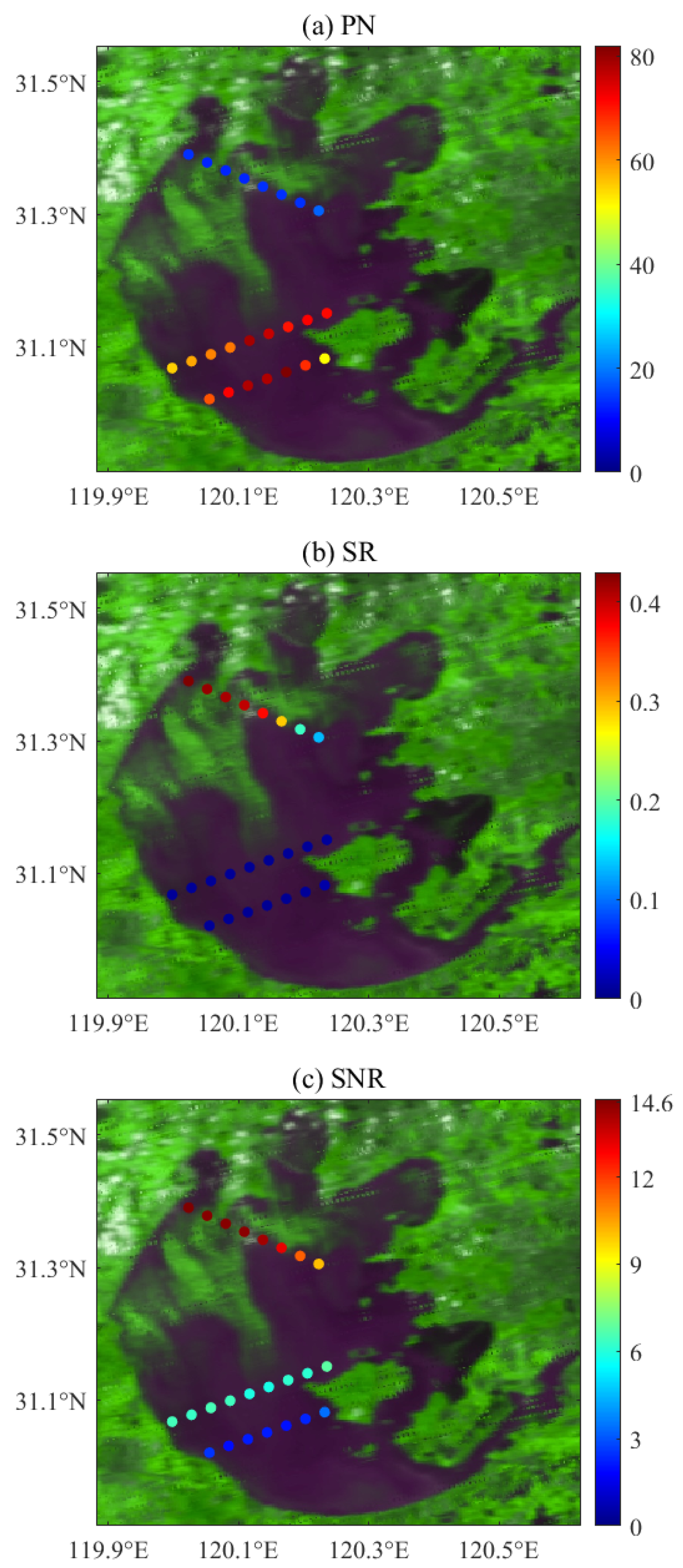
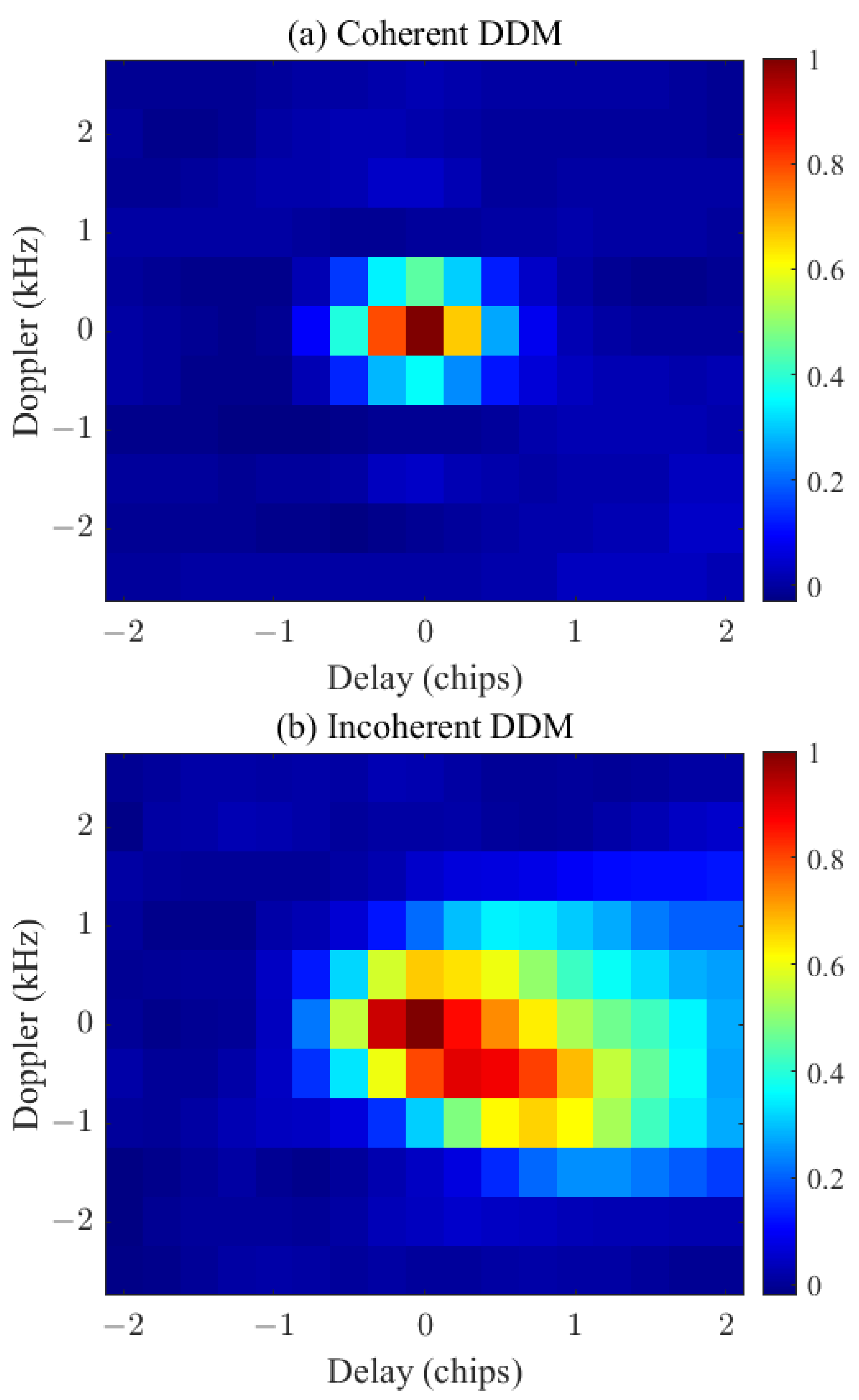
3.1. Employed CYGNSS Observations

GNSS-R is sensitive to the roughness change over lake surfaces, and this change can be seen clearly in the DDMs of CYGNSS (Figure 2). The open water surface tends to be rough when wind blows [41], but when a large-scale floating object exists, it will turn smoother, making the GNSS-R reflected signals coherent [42]. The coherent reflections are easily distinguished through observables extracted from DDMs, which are also the basis of GNSS-R sea ice and oil slick detection.Once the plankton in water reproduce quickly, a kind of green paint-like substance will appear over the water surface, leading to an increase in water surface tension and reduction in the formation of waves, making the GNSS reflected signals coherent. Therefore, monitoring cyanobacteria bloom with the employment of GNSS-R is theoretically feasible. The relationship between the forward scattered GNSS signals and delay-Doppler is represented by a two-dimension function. The maximum power point in the DDM is usually associated with the SP. When the area of SP is covered by cyanobacteria bloom, the reflected GNSS signals are typically coherent, and the power is concentrated near the maximum power point in DDM, but the power will spread into a ‘horseshoe’ shape when the signals come from a rough water surface. In this way, the cyanobacteria bloom can be detected by the observables extracted from DDM (Figure 2).

Based on the reasons above, the pixel number (PN) observable of each DDM, GNSS-R reflectivity (SR, $\Gamma$) and signal-to-noise ratio (SNR) of every CYGNSS data point are selected to detect the suspicious coherent signals from the lake surface. The PN observable, called the DDM spreadness, that can effectively determine the surface roughness surrounding SP sensitively [42], is employed here and defined as the number of pixels with its value > 0.1 in the normalized DDM.

Assuming that the reflected signals are coherent, the surface reflectivity $\Gamma$ is also employed and calculated by [22]

$$\Gamma =\frac{\sigma {(R_t+R_r)}^2}{4\pi {\left(R_t{R}_r\right)}^2},$$

(2)

where $\sigma$ is the bistatic radar cross section, $R_t$ and $R_r$ are the distance from the SP to GNSS satellite and from the SP to CYGNSS satellite, respectively.

The last observable employed is SNR, which can be read directly from the CYGNSS dataset. An approximate correlation between the cyanobacteria bloom condition and the three observables mentioned above can be seen in Figure 1.

3.2. Function of Meteorological Data

Unlike hard sea ice, paint-like cyanobacteria bloom over the water surface is more like oil and usually eases the surface roughness. Such factors as wind speed can affect the reflected GNSS signals by changing the surface roughness. In other words, the presence of low wind speed or cyanobacteria bloom can either lead to smooth surface. Therefore, it is beneficial to have access to wind speed data in this situation. Moreover, meteorological factors not only affect the GNSS reflect signals but also perform an important role in the growth and gathering process of cyanobacteria. Meteorological factors mainly contribute to the growth period of the cyanobacteria, and their abrupt change may promote the eruption of the bloom. Here we take the temperature, solar radiation and wind factors as examples. Sufficient solar radiation, suitable temperature, pressure and precipitation are essential to the growth of cyanobacteria [43]. The sudden decrease in wind speed and the abrupt change of wind direction usually lead to the gathering of cyanobacteria because the constant blowing of the wind above a certain speed will increase the dissolved oxygen in the water, which is beneficial for the growth of cyanobacteria, but will block the accumulation of cyanobacteria. Once the wind speed weakens, the grown cyanobacteria have a chance to rise and gather together. The abrupt change of wind direction will inversely affect the water current of the lake surface and will also help the cyanobacteria to rise and gather. Taking the relationship between wind and cyanobacteria [44] into account, meteorological factors are involved as an auxiliary to further confirm the bloom existence with the application of the RUSBoost algorithm. As such, both the remote sensing observation results and cyanobacteria bloom formation mechanism are considered.

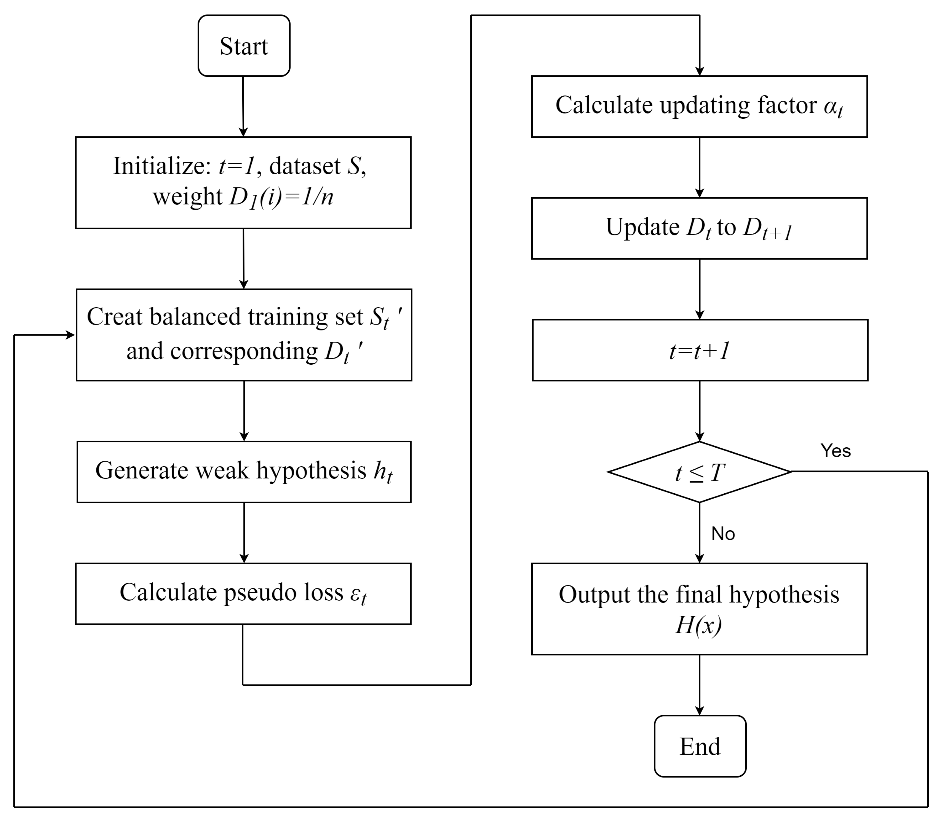
3.3. Classification Algorithm

Throughout most of the observation period, there is no cyanobacteria bloom that occurs over the lake surface, so the training data are an imbalanced dataset, and points without cyanobacteria bloom presence are in the majority class, while those with cyanobacteria bloom are in the minority class but need to be emphasized. To deal with the imbalanced data classification problem, we employ the RUSBoost algorithm. The RUSBoost algorithm targets the minimization of the misclassification rate of each class; instead of pursuing the highest OA, it randomly selects some points from the majority class, with its number being equal to that of the minority class, and then trains weak learners by iterations to adjust the weight of each sample until the goal of classifying the imbalanced datasets is achieved. Firstly, we give an imbalanced dataset S and weights D; S includes n dimensions vector $\mathit{x}=\{x_1,x_2,...,x_i,...,x_n\}$ and class label $y=\{y_1,y_2,...,y_i,...,y_n\}$, $y_i=0$ or 1. The initial weight of each sample is set as $1/n$ in the first iteration ($D_1\left(i\right)=1/n$). In the $t$th iteration of total T iterations, the temporarily balanced dataset $S_t^{{}^{\prime }}\subset S_t$ is created by the RUS method, and the corresponding weights $D_t^{{}^{\prime }}\subset D_t$ are also created at the same time. The next step is using $S_t^{{}^{\prime }}$ and $D_t^{{}^{\prime }}$ to train the weak hypothesis $h_t$ by some classification algorithms, such as WeakLearn. The weak hypothesis performs just a little better than random classification (accuracy around 50%), but combining them together to form a final hypothesis, the classification accuracy is much enhanced. Then, we calculate the pseudo-loss ${ϵ}_t$, while pseudo-loss is computed as the following formula:

$${ϵ}_t=\sum _{i=1}^n{D}_t\left(i\right)(1-h_t(x_i,y_i)+h_t(x_i,1-y_i)).$$

(3)

In every iteration, the weights $D_t$ are updated by the updating factor ${\alpha }_t={ϵ}_t/(1-{ϵ}_t)$:

$$D_{t+1}\left(i\right)=D_t\left(i\right){\alpha }_t^{\frac{1}{2}(1+h_t(x_i,y_i)-h_t(x_i,1-y_i))}.$$

(4)

Then, we normalize $D_{t+1}$ by

$$D_{t+1}\left(i\right)=\frac{D_{t+1}\left(i\right)}{{\sum }_{i=1}^m{D}_{t+1}\left(i\right)}.$$

(5)

By this point, the process of one iteration is finished. If the iteration number t is not bigger than T, the iteration will continue, or it will be stopped. Finally, the output of the final hypothesis $H\left(x\right)$ is formed:

$$H\left(x\right)=\underset{y\in 0,1}{argmax}\sum _{t=1}^T{h}_t(x,y)log\frac{1}{{\alpha }_t}.$$

(6)

All steps of the RUSBoost algorithm are posted in the flowchart (Figure 3); for more detailed information about RUSBoost, refer to [31]. According to the discussions above, a new method for GNSS-R algal bloom detection is proposed, and the flowchart is displayed in Figure 4.

4. Experiments and Evaluation

To prove the effectiveness of GNSS-R data and meteorological data in cyanobacteria bloom detection, as well the superiority of the RUSBoost method, three assessment stages are involved in this section, which are the manual threshold value method classified by the single GNSS-R observable, and the results with/without meteorological factors considered through the ML method and error analysis. Meanwhile, the training and testing process of the RUSBoost algorithm and the performance indexes are also illustrated.

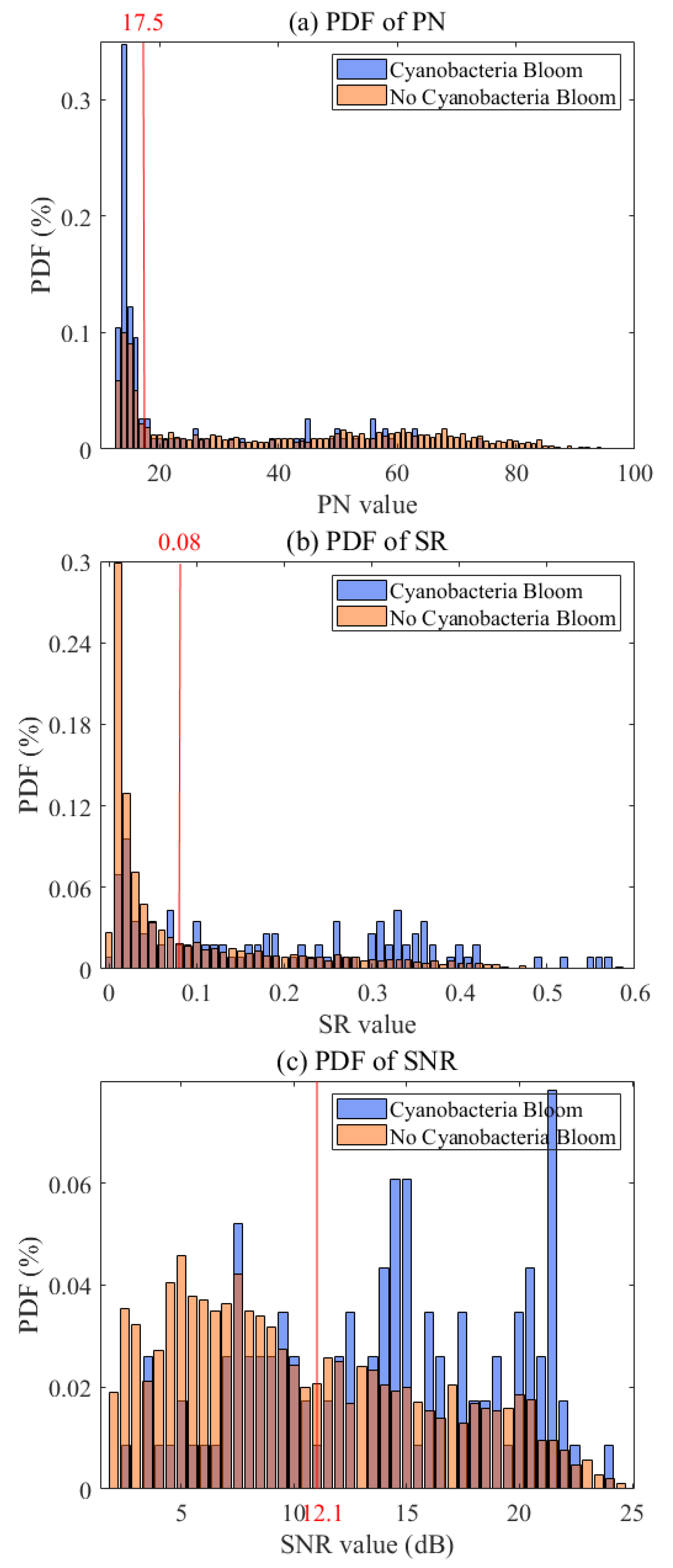
4.1. Threshold Value Method

Figure 5 shows the probability density function (PDF) of the three GNSS-R observables under the circumstance with or without cyanobacteria bloom occurrence. We manually selected a threshold in each PDF to make the classification accuracy relatively the same in each class, and the thresholds are marked by red lines in the PDFs. In the PDF of PN, we expect that the power from points with cyanobacteria bloom coverage is mostly concentrated in the PN values between 10 and 20, as the coherent power of reflected GNSS signals is less spread when the surface is smooth, similar to specular reflection. As we can see in Figure 5a and Table 1, the threshold we selected is 17.5, which generally agrees with our expectation. While in the PDF of SR, the situation is the opposite, the stronger the coherent reflection, the higher the reflectivity. So, the conclusion is readily drawn that the cyanobacteria bloom points tend to show the character of high SR values. Actually, Figure 5b also proves this tendency, and the threshold is set as 0.08. The last GNSS-R observable employed in this paper is SNR; its tendency is similar to SR, but the data distribution of it is more even relative to PN and SR, and the threshold is set as 12.1 dB (Figure 5c). The results of the threshold value classification via PDF are recorded in Table 1. In order to indicate the classification accuracy, we employed the performance indexes including the true positive (TP) rate (TPR), true negative (TN) rate (TNR) and OA. TP and TN refer to the two correctly classified situations, and OA is calculated as follows:

$$OA=\frac{TP+TN}{TP+TN+FP+FN}$$

(7)

These three performance indexes range from 0 to 1, and the closer they are to 1, the better the results. In this method, TPR, TNR and OA are mostly better than 65%, which shows the ability to distinguish cyanobacteria bloom from the clean water surface using GNSS-R observables. However, the accuracy of it is still unsatisfactory, the probable reason being that there are some situations where the surface is calm due to low wind speed instead of actual cyanobacteria bloom, or a strong wind suddenly blows and roughens the lake surface but the cyanobacteria bloom is not blown away. To better fix these mistakes, a scheme is designed to combine GNSS-R data and meteorological data with the help of the ML method.

Figure 5. PDFs of three GNSS-R observables with cyanobacteria bloom covered or not, red lines and numbers refer to the classification threshold.

Figure 5. PDFs of three GNSS-R observables with cyanobacteria bloom covered or not, red lines and numbers refer to the classification threshold.

Table 1. Results of threshold value method for three GNSS-R observables.

	PN	SR	SNR
Threshold	17.5	0.08	12.1
TNR	69.6%	66.8%	64.5%
TPR	67.9%	67.0%	63.5%
OA	0.68	0.67	0.64

Table 1. Results of threshold value method for three GNSS-R observables.

	PN	SR	SNR
Threshold	17.5	0.08	12.1
TNR	69.6%	66.8%	64.5%
TPR	67.9%	67.0%	63.5%
OA	0.68	0.67	0.64

4.2. Machine Learning Method

4.2.1. Training

After data quality control and collocation, 2913 samples were obtained in total in the training procession, 1942 of which were used while the remaining 971 were used for testing. Three GNSS-R observables and six kinds of meteorological factors were input to the classifier as features; the samples with bloom coverage (NDVI > 0.05) were labeled as 1 or 0 for bloom or no bloom, respectively. The RUSBoost algorithm was realized through the Classification Learner in the Machine Learning and Deep Learning Toolbox of MATLAB R2021b. The numbers of weak learners, learning rate and the cost of misclassification were set as 100, 0.1 and 1, respectively, as they performed the best during exhaustive tests.

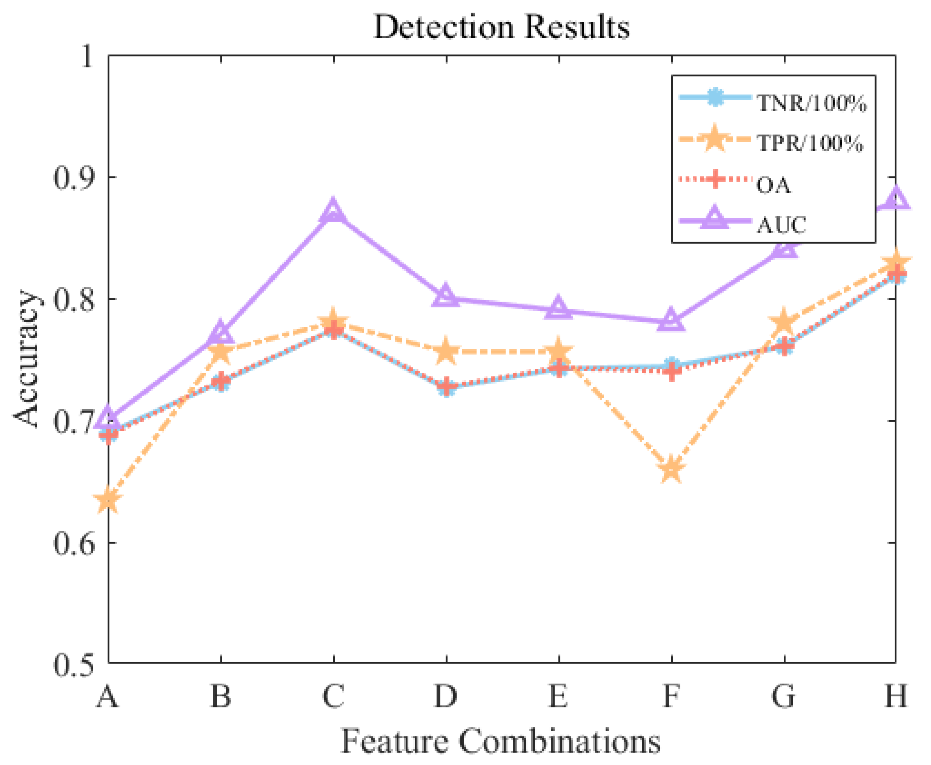
4.2.2. Detection Results

Another performance index suitable for evaluating the imbalanced data classification effect is area under curve (AUC), also employed here for evaluating the performance of the RUSBoost algorithm. In addition, AUC is an indicator calculated from the receiver operating characteristic curve (ROC; it is in the coordinate system where the TPR is on the y-axis and the false positive rate (FPR) is on the x-axis [45]), which is the size of the area under ROC and also shows the performance of the classifier. The detection results of different feature combinations are listed in

Table 2. Test results of different feature combinations.

	Combination	Results	Acuracy	OA	AUC
A	GNSS-R	TNR	68.9%	0.69	0.70
		TPR	63.4%
B	GNSS-R + WS	TNR	73.1%	0.73	0.77
		TPR	75.6%
C	GNSS-R + T	TNR	77.4%	0.77	0.87
		TPR	78.0%
D	GNSS-R + P	TNR	72.6%	0.73	0.80
		TPR	75.6%
E	GNSS-R + ToP	TNR	74.2%	0.74	0.79
		TPR	75.6%
F	GNSS-R + WD	TNR	74.4%	0.74	0.78
		TPR	65.9%
G	GNSS-R + SRD	TNR	76.0%	0.76	0.84
		TPR	78.0%
H	All Features	TNR	81.9%	0.82	0.88
		TPR	82.9%

, and the visualization of Table 2 is shown in Figure 6. We considered eight different feature combinations, and they can be roughly divided into three groups: only GNSS-R observables (combination A in Table 2); GNSS-R observables + all employed meteorological factors (combination H); and GNSS-R observables + one of the employed meteorological factors (combinations B-G). In these three groups, one can come to the conclusion that the involvement of meteorological factors can apparently improve the detection accuracy, while the contributions of each meteorological factor are varied. When no meteorological factors are involved, the accuracy results for cyanobacteria bloom detection (TPR), clean lake surface detection (TNR), OA and AUC are 63.4%, 68.9%, 68.7% and 0.70, respectively. Compared with the threshold value method used before, there is almost no significant improvement in the combination of the three observables, but the application potential of GNSS-R in this field can still be proven because the AUC value here is greater than 0.5, which indicates the effectiveness of the imbalanced data classification. After all the meteorological factors were engaged, the performance indexes improved a lot and were able to reach 81.9%, 82.9%, 82.0% and 0.88 in the four performance indexes, respectively, gaining 10–20% more than before, showing the prospect of the GNSS-R cyanobacteria bloom detection method by taking meteorological factors into consideration. Through doing so, some disturbing factors are excluded. For instance, on one certain day, the wind speed is quite low, so the coherent reflection from the lake surface is received such that it looks like cyanobacteria bloom exists, but the temperature on this day, or in the period ten days before, is lower than 10 °C (which hinders cyanobacteria growth), so the possibility of cyanobacteria bloom occurrence can be ruled out. This proposed method effectively overcomes the shortcomings of GNSS-R data (failure to identify the actual reason that leads to the smoothness of the lake surface). Then, the contributions by single meteorological factor to the final result were evaluated. In Table 2 and Figure 6, the performance of combination B-G is better than that of combination A but worse than that of combination H. This means that the six meteorological factors involved are effective in the research, and considering all of them can produce the best result. Temperature (combination C) and solar radiation (combination G) contribute most compared to other factors. The two combinations improve by 8.7%, 7.4% in OA, 14.6%, 14.6% in TPR, 8.5%, 7.1% in TNR and 0.17, 0.14 in AUC, respectively, relative to combination A. The result that temperature and solar contribute most to cyanobacteria bloom detection fits the conclusion in [43] well, in which it is found that suitable light and temperature are the key factors that affect the growth of cyanobacteria bloom.

4.3. Error Analysis

To better find the error sources in the detection results, we mapped the correctly classified and misclassified points on a day together. Through the observation, we discovered that the misclassified points mostly appear near the edge of the actual cyanobacteria bloom-covered zone. On 30 May 2021, cyanobacteria accumulated and covered almost the entire lake (Figure 7a). On this day, 11 CYGNSS points were available in the test dataset, and they all correctly classified as positive for the existence of cyanobacteria bloom, showing the great accuracy of the proposed method. On the days that nearly no cyanobacteria bloom occurred, such as 17 August 2020 (Figure 7b), the detection results are also satisfactory, and mistakes are seldom seen in this situation. Therefore, we conclude that the detection accuracy of this method is reliable when the surface condition is rather uniform (no cyanobacteria bloom or massive coverage). As Figure 7c shows, our method also shows the ability to identify the cyanobacteria bloom zone to a certain degree when a small amount of cyanobacteria bloom exists. Misclassification usually occurs when the lake is partially covered by cyanobacteria bloom. We take 22 May 2019 and 11 October 2020 (Figure 7d,e) as examples where half of the total points are classified incorrectly (3/7 and 4/8, respectively). By inspecting the misclassified point locations with the cyanobacteria bloom area on that day, the misclassified points usually are located not far away from the cyanobacteria bloom zone, which covers a considerable area of the lake. We speculate that the probable reason for it is that the cyanobacteria bloom zone nearby not only limits the wave height in the zone itself but also the surrounding area, even the whole lake. Although this situation is a kind of misclassification, it does not influence the application value of this method seriously, as it can detect the possible cyanobacteria bloom existence in the lake, especially for some real-world applications, where exact edge information is not required. Relative to optical remote sensing data, it has progressed a lot since this method can warn of the dangers of cyanobacteria bloom occurrence during overcast weather, but optical data are not accessible. Another kind of misclassification is from the confusing weather conditions. On 23 May 2019 (Figure 7f), most points are judged incorrectly (11/13). On this day, only some parts of the lake surface are covered by cyanobacteria bloom, but the average wind speed near the SPs is mostly less than 3 m/s, leading to coherent reflection from the lake surface, while the average wind speed ten days before the day is around 3.5 m/s. The average temperature is more than 21 °C, and the average atmosphere pressure is around 1010 hpa on the observing day and ten days before, which are generally suitable for the growth and gathering of cyanobacteria, but not much cyanobacteria bloom actually emerges. This phenomenon is not usual in the research period. It needs to be pointed out that despite the involvement of meteorological factors successfully reducing the misclassification to a large extent, they still cannot overcome it completely. More countermeasures remain to be proposed in the future to further decrease the misclassification rate of GNSS-R algal bloom detection.

5. Conclusions

This research presents a machine learning algorithm-based GNSS-R algal bloom detection method with auxiliary meteorological data. GNSS-R observables extracted from CYGNSS DDMs and meteorological factors are selected as input to the RUSBoost model, an algorithm designed for classifying imbalanced datasets. In the beginning, we proved the feasibility of detecting algal bloom by a single GNSS-R observable using the manual threshold value method and achieved a detection accuracy around 65%. To pursue further improvement in the detection results, we introduced meteorological reanalysis data of ERA5-Land and the ML method. By comparing different feature combinations, we can conclude that with the aid of meteorological factors, the detection accuracy can be improved to a relatively great extent, especially when all the meteorological factors we considered are involved (test TPR = 82.9%, TNR = 81.9%, OA = 82.0% and AUC = 0.88). The influence of different meteorological factors on the final result was also evaluated. Among all other factors, temperature and solar radiation downwards have the best correlation with the bloom conditions, with improvements of around 10% being observed in the results, though lower than the feature combination containing all meteorological factors. Finally, we discussed the performance of the proposed method under different surface conditions and the probable reason for the mistakes in the detection results, and found that when the lake surface is rather uniform (nearly full of algal bloom or with no bloom), the performance is plausible, while on days where the lake surface is partly covered by algal bloom, the mistake rate increases. Moreover, there are still some conditions in which GNSS-R and meteorological data are not enough to successfully distinguish the existence of algal bloom.

Some problems remain to be solved in the future. The detection accuracy needs to be further progressed, which may be realized by applying other ML methods, and more features can be considered. Besides this, the employment of meteorological reanalysis data in this research represents the mechanism of algal bloom growth and dissolves the uncertainty by GNSS-R coherent detection. For comparison, the measured in situ meteorological data can be utilized, and the performance between the measured data and that of ERA5-Land reanalysis data should be discussed. After the classification method becomes mature, regression analysis will be conducted.

References

1. Xie, R.; Pang, Y.; Bao, K. Spatiotemporal distribution of water environmental capacity-a case study on the western areas of Taihu Lake in Jiangsu Province, China. Environ. Sci. Pollut. Res. 2014, 21, 5465–5473. [Google Scholar] [CrossRef] [PubMed]
2. Cheng, X.; Li, S. An analysis on the evolvement processes of lake eutrophication and their characteristics of the typical lakes in the middle and lower reaches of Yangtze River. Chin. Sci. Bull. 2006, 51, 1603–1613. [Google Scholar] [CrossRef]
3. Wu, J.Y.; Xu, Q.J.; Gao, G.; Shen, J.H. Evaluating genotoxicity associated with microcystin-LR and its risk to source water safety in Meiliang Bay, Taihu Lake. Environ. Toxicol. 2006, 21, 250–255. [Google Scholar] [CrossRef] [PubMed]
4. Hu, C.; Lee, Z.; Ma, R.; Yu, K.; Li, D.; Shang, S. Moderate resolution imaging spectroradiometer (MODIS) observations of cyanobacteria blooms in Taihu Lake, China. J. Geophys. Res. Ocean. 2010, 115, C04002. [Google Scholar] [CrossRef] [Green Version]
5. Hilborn, E.D.; Beasley, V.R. One health and cyanobacteria in freshwater systems: Animal illnesses and deaths are sentinel events for human health risks. Toxins 2015, 7, 1374–1395. [Google Scholar] [CrossRef] [Green Version]
6. Zhang, T.; Hu, H.; Ma, X.; Zhang, Y. Long-term spatiotemporal variation and environmental driving forces analyses of algal blooms in Taihu lake based on multi-source satellite and land observations. Water 2020, 12, 1035. [Google Scholar] [CrossRef] [Green Version]
7. Klemas, V. Remote sensing of algal blooms: An overview with case studies. J. Coast. Res. 2012, 28, 34–43. [Google Scholar] [CrossRef]
8. Wang, L.; Xu, X.; Yu, Y.; Yang, R.; Gui, R.; Xu, Z.; Pu, F. SAR-to-optical image translation using supervised cycle-consistent adversarial networks. IEEE Access 2019, 7, 129136–129149. [Google Scholar] [CrossRef]
9. Dhillon, M.S.; Dahms, T.; Kübert-Flock, C.; Steffan-Dewenter, I.; Zhang, J.; Ullmann, T. Spatiotemporal Fusion Modelling Using STARFM: Examples of Landsat 8 and Sentinel-2 NDVI in Bavaria. Remote Sens. 2022, 14, 677. [Google Scholar] [CrossRef]
10. Wang, G.; Li, J.; Zhang, B.; Shen, Q.; Zhang, F. Monitoring cyanobacteria-dominant algal blooms in eutrophicated Taihu Lake in China with synthetic aperture radar images. Chin. J. Oceanol. Limnol. 2015, 33, 139–148. [Google Scholar] [CrossRef]
11. Ghasemigoudarzi, P.; Huang, W.; Silva, O.D.; Yan, Q.; Power, D.T. Flash flood detection from CYGNSS data using the RUSBoost algorithm. IEEE Access 2020, 8, 171864–171881. [Google Scholar] [CrossRef]
12. Papale, D.; Belli, C.; Gioli, B.; Miglietta, F.; Ronchi, C.; Vaccari, F.P.; Valentini, R. ASPIS, a flexible multispectral system for airborne remote sensing environmental applications. Sensors 2008, 8, 3240–3256. [Google Scholar] [CrossRef] [PubMed] [Green Version]
13. Li, W.; Cardellach, E.; Fabra, F.; Rius, A.; Ribó, S.; Martín-Neira, M. First spaceborne phase altimetry over sea ice using TechDemoSat-1 GNSS-R signals. Geophys. Res. Lett. 2017, 44, 8369–8376. [Google Scholar] [CrossRef]
14. Yan, Q.; Huang, W. Sea Ice Thickness Measurement Using Spaceborne GNSS-R: First Results with TechDemoSat-1 Data. IEEE J. Sel. Top. Appl. Earth Obs. Remote Sens. 2020, 13, 577–587. [Google Scholar] [CrossRef]
15. Zhu, Y.; Tao, T.; Yu, K.; Qu, X.; Li, S.; Wickert, J.; Semmling, M. Machine learning-aided sea ice monitoring using feature sequences extracted from spaceborne gnss-reflectometry data. Remote Sens. 2020, 12, 3751. [Google Scholar] [CrossRef]
16. Wei, H.; Yu, T.; Tu, J.; Ke, F. Detection and Evaluation of Flood Inundation Using CYGNSS Data during Extreme Precipitation in 2022 in Guangdong Province, China. Remote Sens. 2023, 15, 297. [Google Scholar] [CrossRef]
17. Yan, Q.; Chen, Y.; Jin, S.; Liu, S.; Jia, Y.; Zhen, Y.; Chen, T.; Huang, W. Inland Water Mapping Based on GA-LinkNet from CyGNSS Data. IEEE Geosci. Remote Sens. Lett. 2023, 20, 1500305. [Google Scholar] [CrossRef]
18. Ruf, C.S.; Balasubramaniam, R. Development of the CYGNSS Geophysical Model Function for Wind Speed. IEEE J. Sel. Top. Appl. Earth Obs. Remote Sens. 2019, 12, 66–77. [Google Scholar] [CrossRef]
19. Reynolds, J.; Clarizia, M.P.; Santi, E. Wind Speed Estimation from CYGNSS Using Artificial Neural Networks. IEEE J. Sel. Top. Appl. Earth Obs. Remote Sens. 2020, 13, 708–716. [Google Scholar] [CrossRef]
20. Yan, Q.; Huang, W.; Jin, S.; Jia, Y. Pan-tropical soil moisture mapping based on a three-layer model from CYGNSS GNSS-R data. Remote Sens. Environ. 2020, 247, 111944. [Google Scholar] [CrossRef]
21. Edokossi, K.; Calabia, A.; Jin, S.; Molina, I. GNSS-reflectometry and remote sensing of soil moisture: A review of measurement techniques, methods, and applications. Remote Sens. 2020, 12, 614. [Google Scholar] [CrossRef] [Green Version]
22. Chew, C.C.; Small, E.E. Soil Moisture Sensing Using Spaceborne GNSS Reflections: Comparison of CYGNSS Reflectivity to SMAP Soil Moisture. Geophys. Res. Lett. 2018, 45, 4049–4057. [Google Scholar] [CrossRef] [Green Version]
23. Rodriguez-Alvarez, N.; Oudrhiri, K. The bistatic radar as an effective tool for detecting and monitoring the presence of phytoplankton on the ocean surface. Remote Sens. 2021, 13, 2248. [Google Scholar] [CrossRef]
24. Ban, W.; Zhang, K.; Yu, K.; Zheng, N.; Chen, S. Detection of Red Tide over Sea Surface Using GNSS-R Spaceborne Observations. IEEE Trans. Geosci. Remote Sens. 2022, 60, 5802911. [Google Scholar] [CrossRef]
25. Zhang, Y.; Wang, Y.; Zhou, S.; Meng, W.; Han, Y.; Yang, S. Feasibility study of spaceborne GNSS-R detection of algal blooms in Taihu Lake. J. Beijing Univ. Aeronaut. Astronaut. 2022, 13, 1–14. [Google Scholar]
26. Lary, D.J.; Alavi, A.H.; Gandomi, A.H.; Walker, A.L. Machine learning in geosciences and remote sensing. Geosci. Front. 2016, 7, 3–10. [Google Scholar] [CrossRef] [Green Version]
27. Maxwell, A.E.; Warner, T.A.; Fang, F. Implementation of machine-learning classification in remote sensing: An applied review. Int. J. Remote Sens. 2018, 39, 2784–2817. [Google Scholar] [CrossRef] [Green Version]
28. Yan, Q.; Huang, W.; Moloney, C. Neural Networks Based Sea Ice Detection and Concentration Retrieval from GNSS-R Delay-Doppler Maps. IEEE J. Sel. Top. Appl. Earth Obs. Remote Sens. 2017, 10, 3789–3798. [Google Scholar] [CrossRef]
29. Zhu, Y.; Wickert, J.; Tao, T.; Yu, K.; Li, Z.; Qu, X.; Ye, Z.; Geng, J.; Zou, J.; Semmling, M. Sensing Sea Ice Based on Doppler Spread Analysis of Spaceborne GNSS-R Data. IEEE J. Sel. Top. Appl. Earth Obs. Remote Sens. 2020, 13, 217–226. [Google Scholar] [CrossRef]
30. Jia, Y.; Jin, S.; Yan, Q.; Savi, P. The Sensitivity Analysis on GNSS-R Soil Moisture Retrieval. In Proceedings of the 2021 Photonics & Electromagnetics Research Symposium (PIERS), Hangzhou, China, 21–25 November 2021; pp. 2307–2311. [Google Scholar]
31. Seiffert, C.; Khoshgoftaar, T.M.; Hulse, J.V.; Napolitano, A. RUSBoost: A hybrid approach to alleviating class imbalance. IEEE Trans. Syst. Man Cybern. Part A Syst. Hum. 2010, 40, 185–197. [Google Scholar] [CrossRef]
32. Freund, Y.; Schapire, R.E. Experiments with a New Boosting Algorithm; Morgan Kaufmann Publishers Inc.: San Francisco, CA, USA, 1996; pp. 1–14. [Google Scholar]
33. Cheng, L.; Xue, B.; Zawisza, E.; Yao, S.; Liu, J.; Li, L. Effects of environmental change on subfossil Cladocera in the subtropical shallow freshwater East Taihu Lake, China. Catena 2020, 188, 104446. [Google Scholar] [CrossRef]
34. Tao, Y.; Zhang, Y.; Meng, W.; Hu, X. Characterization of heavy metals in water and sediments in Taihu Lake, China. Environ. Monit. Assess. 2012, 184, 4367–4382. [Google Scholar] [CrossRef] [PubMed]
35. Zhong, J.; Chengxin, C.F.; Liu, G.; Zhang, L.; Shang, J.; Gu, X. Seasonal variation of potential denitrification rates of surface sediment from Meiliang Bay, Taihu Lake, China. J. Environ. Sci. 2010, 22, 961–967. [Google Scholar] [CrossRef]
36. Zou, H.; Pan, G.; Chen, H.; Yuan, X. Removal of cyanobacterial blooms in Taihu Lake using local soils. II. Effective removal of Microcystis aeruginosa using local soils and sediments modified by chitosan. Environ. Pollut. 2006, 141, 201–205. [Google Scholar] [CrossRef]
37. Ruf, C.S.; Chew, C.; Lang, T.; Morris, M.G.; Nave, K.; Ridley, A.; Balasubramaniam, R. A New Paradigm in Earth Environmental Monitoring with the CYGNSS Small Satellite Constellation. Sci. Rep. 2018, 8, 8782. [Google Scholar] [CrossRef] [PubMed] [Green Version]
38. Wang, J.; Hu, Y.; Li, Z. A New Coherence Detection Method for Mapping Inland Water Bodies Using CYGNSS Data. Remote Sens. 2022, 14, 3195. [Google Scholar] [CrossRef]
39. Cao, B.; Gruber, S.; Zheng, D.; Li, X. The ERA5-Land soil temperature bias in permafrost regions. Cryosphere 2020, 14, 2581–2595. [Google Scholar] [CrossRef]
40. Soares, P.M.; Lima, D.C.; Nogueira, M. Global offshore wind energy resources using the new ERA-5 reanalysis. Environ. Res. Lett. 2020, 15, 1040a2. [Google Scholar] [CrossRef]
41. Loria, E.; O’Brien, A.; Zavorotny, V.; Zuffada, C. Towards Wind Vector and Wave Height Retrievals Over Inland Waters Using CYGNSS. Earth Space Sci. 2021, 8, e2020EA001506. [Google Scholar] [CrossRef]
42. Yan, Q.; Huang, W. Spaceborne GNSS-R Sea Ice Detection Using Delay-Doppler Maps: First Results from the U.K. TechDemoSat-1 Mission. IEEE J. Sel. Top. Appl. Earth Obs. Remote Sens. 2016, 9, 4795–4801. [Google Scholar] [CrossRef]
43. Zhou, B.; Cai, X.; Wang, S.; Yang, X. Analysis of the Causes of Cyanobacteria Bloom: A Review. J. Resour. Ecol. 2020, 11, 405. [Google Scholar]
44. Qi, L.; Hu, C.; Visser, P.M.; Ma, R. Diurnal changes of cyanobacteria blooms in Taihu Lake as derived from GOCI observations. Limnol. Oceanogr. 2018, 63, 1711–1726. [Google Scholar] [CrossRef] [Green Version]
45. Provost, F.; Org, P.; Fawcett, T. Robust Classification for Imprecise Environments. Mach. Learn. 2000, 42, 203–231. [Google Scholar]
Figure 1. MODIS image of Taihu Lake on 17 September 2021 and the response of three GNSS-R observables (introduced in Section 3.1), where the lake surface is covered by cyanobacteria bloom or not.
Remotesensing 15 03122 g001
Figure 2. (a) Typical DDMs with SP on cyanobacteria bloom and (b) on normal lake surface.
Remotesensing 15 03122 g002
Figure 3. Flowchart of RUSBoost algorithm.
Remotesensing 15 03122 g003
Figure 4. Flowchart of this research. Blue boxes are the processing steps about CYGNSS data, orange box is about ERA5-Land data, red boxes are about MODIS data and green boxes are the modeling and evaluation steps.
Remotesensing 15 03122 g004
Figure 6. Line chart of the results in Table 2. The letters at the botton of the figure refer to the feature combinations in Table 2.
Remotesensing 15 03122 g006
Figure 7. Detection results on different days during the research period, where green area is cyanobacteria bloom coverage (NDVI > 0.05), and red points are the SPs being classified correctly, while the red crosses are misclassified.
Remotesensing 15 03122 g007