Abstract
Accurate land cover classification (LCC) is essential for studying global change. Synthetic aperture radar (SAR) has been used for LCC due to its advantage of weather independence. In particular, the dual-polarization (dual-pol) SAR data have a wider coverage and are easier to obtain, which provides an unprecedented opportunity for LCC. However, the dual-pol SAR data have a weak discrimination ability due to limited polarization information. Moreover, the complex imaging mechanism leads to the speckle noise of SAR images, which also decreases the accuracy of SAR LCC. To address the above issues, an improved dual-pol radar vegetation index based on multiple components (DpRVIm) and a new LCC method are proposed for dual-pol SAR data. Firstly, in the DpRVIm, the scattering information of polarization and terrain factors were considered to improve the separability of ground objects for dual-pol data. Then, the Jeffries-Matusita (J-M) distance and one-dimensional convolutional neural network (1DCNN) algorithm were used to analyze the effect of difference dual-pol radar vegetation indexes on LCC. Finally, in order to reduce the influence of the speckle noise, a two-stage LCC method, the 1DCNN-MRF, based on the 1DCNN and Markov random field (MRF) was designed considering the spatial information of ground objects. In this study, the HH-HV model data of the Gaofen-3 satellite in the Dongting Lake area were used, and the results showed that: (1) Through the combination of the backscatter coefficient and dual-pol radar vegetation indexes based on the polarization decomposition technique, the accuracy of LCC can be improved compared with the single backscatter coefficient. (2) The DpRVIm was more conducive to improving the accuracy of LCC than the classic dual-pol radar vegetation index (DpRVI) and radar vegetation index (RVI), especially for farmland and forest. (3) Compared with the classic machine learning methods K-nearest neighbor (KNN), random forest (RF), and the 1DCNN, the designed 1DCNN-MRF achieved the highest accuracy, with an overall accuracy (OA) score of 81.76% and a Kappa coefficient (Kappa) score of 0.74. This study indicated the application potential of the polarization decomposition technique and DEM in enhancing the separability of different land cover types in SAR LCC. Furthermore, it demonstrated that the combination of deep learning networks and MRF is suitable to suppress the influence of speckle noise.
1. Introduction
Land cover classification (LCC) provides an important basis for global ecological surveys and sustainable development studies. It also plays an essential role in the study of human–nature interactions [1,2]. With city expansion and forest area reduction, the land cover changes rapidly [3,4]. Hence, timely and accurate LCC is one of the most-important applications in satellite remote sensing [5,6,7,8].
SAR images have become an important data source to produce land cover maps by virtue of their advantages of being independent of weather and having a wide swath [9,10]. The common polarization modes for SAR data are full-polarization, dual-polarization, and single-polarization [11,12]. Although full-polarization mode is more beneficial for extracting information, it has a higher data acquisition cost. Compared with fully polarized SAR data, the dual-polarization (dual-pol) SAR data have wider coverage, but less polarization information. Recently, due to the increasing availability of dual-pol SAR data, they have been widely used in the field of SAR LCC [13,14]. However, the dual-pol SAR data are relatively difficult to interpret not only for the coherent speckle noise, but also for the small backscattering coefficient differences among different land cover types for less polarization mode [15,16]. Therefore, researchers are widely concerned with how to improve the accuracy of LCC for dual-pol SAR data [17,18].
One of the main challenges related to the exploitation of dual-pol SAR data in LCC is how to mine features [19,20], which can improve the separability of land cover types [21]. Recently, some researchers used the scattering randomness of the vegetation structure to calculate the radar vegetation index to enrich SAR features [22,23]. For example, Periasamy (2018) devised the dual-pol SAR vegetation index (DPSVI) based on the backscatter coefficient of and images [24]. Bhogapurapu et al. (2022) devised a new dual-pol SAR vegetation descriptor, the DpRVIc, based on the co-polarized purity component of the wave [25]. The polarization decomposition technique is an effective approach to extract polarization scattering characteristics, which is conducive to revealing the physical mechanism of different land cover types [26,27,28]. Therefore, other researchers tried to introduce the parameters extracted by polarization decomposition to calculate the radar vegetation index [29,30]. Mandal et al. (2020) proposed a new vegetation index, the DpRVI, from dual-pol SAR based on the degree of polarization and the eigenvalue spectrum [31]. However, these radar vegetation indexes are mostly used for biomass estimation [32], soil moisture inversion [33], forest monitoring [34], crop growth monitoring [35], etc. Although many vegetation indexes have been proposed and applied to vegetation monitoring, the evaluation of different radar vegetation indexes in LCC is not sufficient, especially for dual-pol data. In addition, the combination mode of the radar vegetation index and other information sources for LCC, including digital elevation models (DEMs), still deserves discussion.
A robust and efficient classification model plays an important role in SAR LCC. Classic machine learning algorithms are widely used in LCC [36,37,38], such as support vector machine (SVM) [39], random forest (RF) [40], and the artificial neural network (ANN) [41]. Recently, deep learning methods have become an alternative choice for LCC due to their excellent feature-extraction capabilities [42,43]. For example, Solórzano et al. (2021) used U-Net for LCC and obtained higher accuracy for almost all land cover types compared to RF [44]. He et al. (2020) proposed a PolSAR image classification algorithm based on fully convolutional networks (FCNs), which showed excellent classification performance [45]. Mei et al. (2017) constructed a five-layer deep convolutional neural network (C-CNN) to study its ability to learn features [46]. However, all of these methods are pixel-level, so their accuracy is easily influenced by the speckle noise of SAR images. To suppress the speckle noise, there are many suppression algorithms in the image preprocessing, such as Lee filtering and Gamma filtering [47,48]. However, the problem of a low signal-to-noise ratio still exists, which affects the accuracy of LCC, especially the pixel-level classification algorithm. Therefore, the noise robustness is very important for the SAR LCC algorithm.
To deal with the land-cover-mapping task for dual-pol data, with the aim of high precision, we propose an improved dual-pol radar vegetation index based on multiple components (DpRVIm) and designed a new two-stage classification algorithm with Gaofen-3 (GF-3). First of all, this study extracted the backscatter coefficient, polarization entropy, and other features from the dual-pol (HH-HV) GF-3 data and proposed a new radar vegetation index based on them. Then, using the J-M distance and 1DCNN algorithm, the influence of differential dual-pol radar vegetation indexes on LCC was analyzed, and the best combination of features was obtained. Finally, a two-stage classification structure approach combining the 1DCNN and MRF (1DCNN-MRF) was developed, to take advantage of deep learning in feature mining and reduce the impact of coherent speckle noise. The main contributions of this paper are as follows:
- Deriving a new radar vegetation index based on multiple components from dual-pol SAR data. The index, based on the acquisition of polarization information, also takes into account the important influence of elevation on the land cover distribution, which can improve the separability of different land cover types in the scenario using dual-polarization data.
- Proposing an effective SAR LCC method 1DCNN-MRF, in which the 1DCNN classification result is fed into the MRF as the initial label. The method takes full account of the spatial contextual information and has strong noise immunity, while retaining the advantages of deep learning algorithms in feature mining.
To verify the efficiency of the method, GF-3 data under HH-HV polarization mode were selected in this paper. The results showed that the proposed DpRVIm had better separability compared with the classical dual-pol radar vegetation index. The 1DCNN-MRF method proposed in this paper can obtain a better ground classification accuracy compared with the classic pixel-based classification method, and the accuracy can reach 81.76%, which shows the broad application prospects of the method in the field of LCC.
2. Study Area and Data
2.1. Study Area
The research area is part of the Dongting Lake region (112°31′19″E–113°34′1″E, 28°1′59″N–29°59′27″N), as shown in Figure 1. It includes part of Honghu City, Changsha City, and Yueyang City and is located on the border of Hunan Province. The elevation of the study area ranges from 0 m to 772 m. There are mainly plains in the northwest of the study area, while a large number of hills and mountains are distributed in the southeast. The Dongting Lake region belongs to a humid continental monsoon climate with an average annual rainfall fluctuating around 1400 mm [49,50]. The region has many rivers and abundant water resources. There is a diverse mix of land cover types in the study area, which is suitable to carry out research on LCC. In this study, the types of ground objects were divided into urban, water, farmland, and forest.
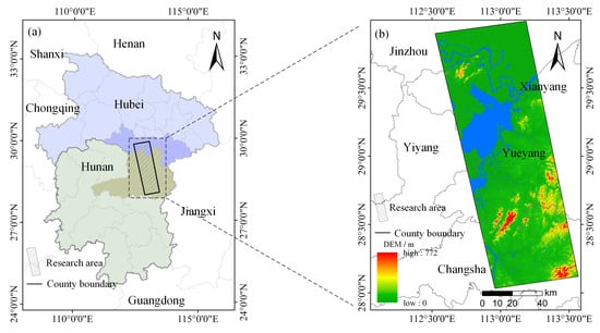
Figure 1.
(a) Location map of the study area; (b) topographic map of the study area.
2.2. Data and Preprocessing
GF-3 is a C-band (SAR) satellite launched by China, with a resolution range of 1–100 m and 12 imaging modes, which can monitor land and sea in any weather conditions and obtain reliable and stable high-resolution SAR images. In this paper, Fine Stripe II mode with a resolution of 10 m was adopted. Furthermore, most current research on the application of the dual-pol radar vegetation index is based on the VV-VH polarization mode, due to the land response of the horizontally polarized transmission wave possibly being different from that of the vertically polarized transmission wave, and the role of the features in the HH-HV mode is less studied. Therefore, the HH-HV model was chosen in this paper to further analyze the role of different features. The specific imaging parameters are shown in Table 1.

Table 1.
Parameters for GF-3.
In this study, the international SAR data processing software PIE-SAR 6.3, which was developed in China, was used to process the GF-3 data [51], specifically: (1) orbit file application; (2) calibration; the backscatter amplitude information on the different polarization channels was corrected according to the calibration constants in the header file to obtain the backscatter coefficient for each pixel; (3) generate polarized covariance matrix; (4) multi-looking; (5) refined Lee filtering; a 3 × 3 fine Lee filtering was used to reduce the influence of speckle noise; (6) polarization decomposition; (7) range Doppler terrain correction; (8) conversion of the backscatter coefficient from a linear to a dB scale; (9) reprojection; (10) study area extraction.
The DEM is a raster digital elevation model obtained by processing remote sensing images, which contain terrain information, which can be used to enrich the interpretation angle of ground objects. The DEM data used in this paper were SRTM v3.0, which has a resolution of 30 m and needs to be resampled to 10 m [52].
2.3. Sample Making
The quantity and quality of samples will affect the LCC accuracy [53,54]. In this study, the land cover samples were made by means of geographical knowledge and visual interpretation. There was a certain degree of cloud coverage in the optical images of the same period, so the optical image dated 12 May 2020 was chosen as the reference data source to help label the samples in this paper. High-resolution remote sensing imagery from Google Earth was used as a secondary data source to correct the samples from areas where the land cover type changed due to temporal inconsistencies. In order to ensure the objectivity of sample selection, a number of representative patches were selected evenly and randomly. Moreover, three interpreters completed the process of visual interpretation independently. When the samples were labeled as different types, the final type of these samples was determined through discussion [55].
The ground objects in the study area were divided into four types: urban, water, farmland, and forest. The existing land cover data for Hunan Province, where the study area is located, had a small proportion of grassland at 0.6%, so there was no separate classification for this category. The position of the land cover samples is shown in Figure 2. The selected 1359 sample patches contained a total of 506,575 pixels. In this study, 50% of them were randomly selected as training samples and the remaining 50% as test samples. The parameters of the samples are shown in Table 2.
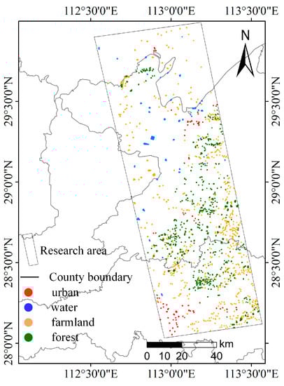
Figure 2.
Distribution map of land cover samples in the study area.
Table 2.
Samples of main ground object types in the study area.
3. Methodology
3.1. Overview
The flow chart of this study on the LCC model is shown in Figure 3. After data collection and preprocessing, the LCC method was mainly divided into three steps. In Step 1, the backscatter coefficients and were extracted, and the DpRVIm was designed and proposed. In Step 2, the J-M distance analysis was performed for each land cover type to select the optimal set of features, and the DpRVIm was analyzed in comparison with the classic radar vegetation index. In Step 3, a new classifier, the 1DCNN-MRF, was designed for LCC and compared with classic machine learning methods such as RF, KNN, and the 1DCNN, giving quantitative and qualitative evaluations.
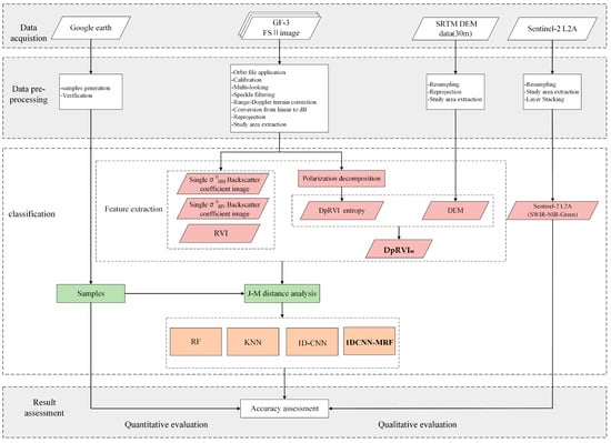
Figure 3.
The flow chart of the proposed land cover classification method.
3.2. Vegetation Index of Dual-Polarization Radar Based on Multiple Components
Using SAR backscatter coefficient features alone is no longer sufficient to obtain high-precision LCC [56]. In this study, a new radar vegetation index based on the multi-component DpRVIm is proposed. The DpRVIm not only allows for the scattering information of polarization and the eigenvalue spectrum, which are used in the DpRVI, but also combines polarization entropy and terrain information. The expression of the DpRVIm is shown in Equation (1).
where (1−mβ) can well characterize the scattering from random targets, including the polarization and eigenvalue spectrum of the scattering information [31]. m is the polarization degree, which is equivalent to the scattered wave anisotropy in dual-pol SAR. It quantifies the relative strength between the first and second dominant scattering mechanisms. β was introduced as the dominant modulation in the scattering mechanism. m and β were calculated as Equations (2) and (3).
where λ1 and λ2 are the normalized eigenvalues from the 2 × 2 covariance matrix C2. C2 is calculated using Equation (4).
where the superscript ∗ denotes the complex conjugate and ⟨⋯⟩ denotes the spatial average over a moving window [31]. This moving window refers to a similar small square pixel block with a certain margin centered on the pixel, and we chose the window size of 5 × 5.
H is the polarized entropy, which characterizes the degree of randomness of the different ground objects. When the value of H is high, the scattering of the target object becomes random noise completely. H is calculated using Equation (5).
where is the probability of the occurrence of each scattering mechanism and represents the eigenvalue of the intensity of this scattering mechanism.
The DEM uses digital elevation data. Topographic relief can affect the distribution of ground objects, and the topographic information contained in the DEM can increase the degree of separation between land types, such as farmland in sloping areas and forest in flat areas. Therefore, the DEM was introduced into the DpRVIm, which can be used to increase the angle of interpreting different ground objects.
Moreover, in order to verify the problems of existing vegetation indexes, the classic indexes, the RVI [57] and DpRVI [31], were chosen in this paper. Their calculation formulae are shown in Table 3.
Table 3.
Formulae of RVI and DpRVI.
3.3. J-M Distance Analysis
In order to fully take advantage of the various features and avoid the interference of ineffective or negative features, we analyzed and filtered the features to derive the optimal feature combinations. After obtaining all the features, we combined them into four feature combinations: the backscatter coefficient, the backscatter coefficient and the RVI, the backscatter coefficient and the DpRVI, and the backscatter coefficient and the DpRVIm. In order to select the feature combination that can better accomplish LCC, the J-M distance analysis method, as shown in Equation (6), was used to analyze the separability of different feature combinations [58,59].
where Dij represents the separability index of the current feature class i and class j and and represent the conditional probability density of feature x belonging to class i and class j, respectively.
The range of Dij was 0–2. It is generally believed that when Dij exceeds 1.9, the sample features between classes i and j have good separability; when Dij is less than 1.5, the sample features between classes i and j are moderately separable; when Dij is less than 1, the sample features between classes i and j are not separable.
3.4. Two-Stage Classification Structure Design
In this study, a two-stage LCC method combining the 1DCNN model and the MRF model was designed. The flow chart of this method is shown in Figure 4. The 1DCNN model has better mining and learning ability for feature information and can apply image features to further improve the quality of LCC. However, the classification of the 1DCNN model is pixel-based, and its results are highly susceptible to the influence of the coherent speckle noise factor of SAR images, which leads to more fragmented land cover type recognition and affects the classification effect. Therefore, in order to reduce the effect of coherent speckle noise, the 1DCNN algorithm was only used to obtain the initial classification result. Then, the initial land cover labels obtained by the 1DCNN and the PCA of features based on dual-pol (HH-HV) data were used as the input of the MRF model to obtain the final land cover map.
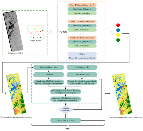
Figure 4.
The flow chart of the two-stage land cover classification model, the 1DCNN-MRF, which is composed of the 1DCNN and MRF.
3.4.1. 1DCNN
As a classic deep learning method, the 1DCNN model includes a convolution module for feature extraction and a classification module for target recognition. In this paper, the designed 1DCNN model contained three one-dimensional convolutional layers. In order to reduce the dimensionality of the local output data of the network, increase the receptive field, and improve the generalization ability of the network structure, a max-pooling layer and a batch normalization layer were added after the convolutional layer. Finally, the one-dimensional feature was used as the input data of the fully connected layer for the classification. The fully connected layer used the activation function “softmax” for the multi-classification and divided the data into four classes.
Three convolutional layers of the model were set with convolutional kernel sizes of 7, 5, and 3, and the number of feature extractors was 32, 64, and 128, respectively. Accordingly, the pooling window size was 2. The feature was fed to the classification module, and then, the preliminary classification result was obtained from the fully connected layer.
3.4.2. MRF
The classification result of 1DCNN was fed into the MRF model as the initial label to form the label field, and the original data were normalized to generate the feature field. Um(f) (Equation (7)) is the feature field energy, which was used to describe the energy value of a pixel belonging to a certain class in the feature field.
where m represents the label number and Xi represents the value of a pixel in the feature field. um is the mean value of pixels belonging to category m, and σ2m is the variance of pixels belonging to category m. um and σ2m are calculated using (8) and (9).
Um(m) (Equation (10)) is the label field energy, which was used to describe the energy value of a pixel belonging to a certain class in the label field.
where β is the potential energy parameter and n(xm) is the number of pixel labels in the neighborhood that are not the same as category m. The neighborhood of a pixel is the eight pixels points around it, also called the eight-neighborhood.
Finally, the total energy (Equation (11)) of the feature fields and label fields was calculated.
The total energy of each pixel belonging to each class was calculated to obtain the class with the minimum energy, and the label field was updated using the minimum energy principle.
4. Result
In this section, firstly, we obtained the numerical distributions of the backscattering coefficient, RVI, DpRVI, and DpRVIm for the four types of land cover: urban, water, farmland, and forest. Secondly, the J-M distance and 1DCNN algorithm were used to analyze the effects of different indexes on LCC and obtain the optimal feature combination. Finally, the classification results of the 1DCNN-MRF were compared with the 1DCNN, KNN, and RF.
4.1. Analysis of Separability of Features
4.1.1. Value Distribution of Features
The values of the samples were used to generate the average value change curves of each feature for different land cover types, as shown in Figure 5. In the numerical distribution of the backscatter coefficient, water had a low backscatter coefficient (Figure 5a,b), which was easier to separate from the other three land types. In addition, the backscatter coefficients of farmland and forest were relatively close to each other, which meant that it was more difficult to distinguish them. As shown in the distribution of the RVI values (Figure 5c), the RVI values of farmland and forest were close to each other, which was still difficult to distinguish, while the types water and urban remained well separable. The distribution of the DpRVI (Figure 5d) values showed a slight increase in the gap between forest and farmland, indicating that forest was easier to distinguish from farmland in the DpRVI compared to the previous three features. The mean values of the DpRVIm (Figure 5e) for different land types were highly variable, with forest being significantly higher than the other three land types. Influenced by the scattering characteristics of the ground, the difference in the values of the DpRVIm between urban and farmland was slightly smaller, while a similar phenomenon also existed in the distribution of the DpRVI. In conclusion, in terms of the numerical distribution, the backscatter coefficient and RVI were advantageous in water and urban extraction, and the DpRVI and the DpRVIm based on polarization decomposition increased the perspective of analyzing ground objects, with better separability between farmland and forest.
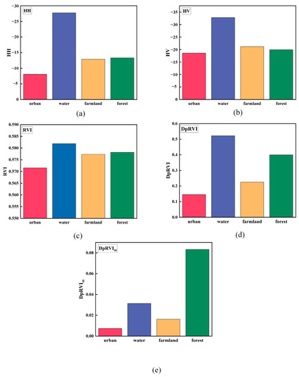
Figure 5.
Distribution of the values of the four different land cover types in terms of different features: (a) ; (b) ; (c) RVI; (d) DpRVI; (e) DpRVIm.
4.1.2. J-M Distance of Different Feature Combinations
In order to analyze the degree of separability of different feature combinations for different land types, we set up four groups of feature combinations. The J-M distances of different land cover types in each feature combination were calculated based on Equation (6).
Figure 6 shows the J-M distances of each feature combination. Among the four groups of feature combinations, the combination of the backscatter coefficient was well distinguished water, while it did so weakly for other land types. Except for water, the J-M distances of other types were all below 1.5, especially for farmland and forest, where the J-M distance was close to 0.5, which means they were hard to separate. After combining the RVI and the DpRVI with the backscattering coefficient, the separability of each land type improved, but the J-M distance between farmland and forest remained below 0.6. After combining the DpRVIm with the SAR backscattering coefficient, the J-M distance values improved for all land types. Specifically, the J-M distance between farmland and forest was obviously enhanced, compared to the RVI and DpRVI. From the result of the J-M distances, the combination of the backscattering coefficient and DpRVIm can effectively enhance the separability of different land cover types. The next step was to further verify the validity of the feature combinations by the classification algorithm.
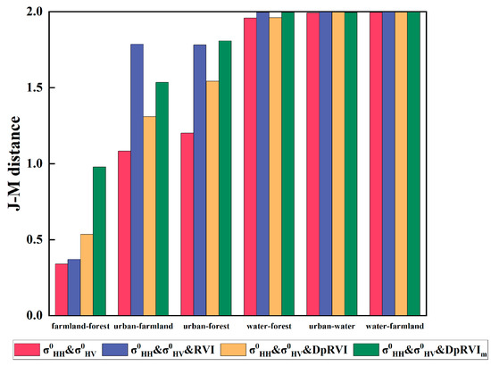
Figure 6.
J-M distances of each feature combination.
4.2. LCC Results Based on Different Feature Combinations
In this section, the quantitative evaluation and the qualitative evaluation of the classification results are presented. The evaluation metrics used in this paper were the overall accuracy (OA), producer’s accuracy (PA), user’s accuracy (UA), and Kappa value. The classification accuracy of the LCC results obtained from different feature combinations based on the 1DCNN method is shown in Table 4. The + + DpRVIm feature combination had the highest accuracy with an OA value of 80.97% and a Kappa value of 0.73, which improved the OA by 3.5% and the Kappa by 5% compared to the + + DpRVI combination. The lowest precision was the + + RVI feature combination with the OA value of 71.23% and the Kappa value of 0.59, which was almost the same as the precision index of the + feature combination. Through the combination of the backscatter coefficient and index based on the polarization decomposition technique, the accuracy of LCC was improved for multiple types compared to the feature combination using the backscatter coefficient alone. In terms of different land cover types, each feature combination showed high accuracy in classifying water, which was related to the scattering characteristics of SAR. In the two feature combinations + + DpRVI and + + DpRVIm, the accuracy of the farmland and forest types significantly improved.
Table 4.
Classification accuracy evaluation of feature combinations.
After the quantitative assessment using the samples, the classification results using different feature combinations were compared with the Sentinel-2 optical images of similar dates to perform a qualitative evaluation of the whole study area. Figure 7a shows the classification results obtained from different feature combinations. It can be seen that the water in all combinations was classified well. This was mainly due to the weak scattering intensity and flat surface of the water, so it was possible to distinguish the water well by using only the combination + . The result of the + + RVI feature combination (Figure 7a(iii)) was closer to that of the + combination (Figure 7a(ii)); both of these combinations had some misclassification of farmland and forest. After the introduction of the DpRVI or DpRVIm, the misclassification of farmland and forest was reduced, among which the DpRVIm had a better effect.
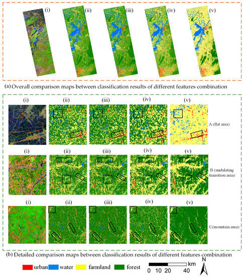
Figure 7.
Classification results of different feature combinations: (i) Sentinel-2A (11-8-3/SWIR-NIR-Green), (ii) + , (iii) + + RVI, (iv) + + DpRVI, (v) + + DpRVIm. (a) Overall comparison maps. (b) Detailed comparison maps.
Figure 7b shows the enlarged classification results of the study area, in which Flat Area A, Undulating Transition Area B, and Mountainous Area C were selected as representative regions. As seen in Flat Area A in Figure 7b, comparing with + , the + + DpRVI feature combination reduced a part of the misclassification of farmland and urban, but some farmland was still wrongly classified as forest. This phenomenon was improved after adding the DpRVIm. From Undulating Transition Area B in Figure 7b, it can be seen that, after adding the DpRVI or DpRVIm, the farmland misclassified as forest was correctly identified, and the phenomenon of farmland omission improved. As can be seen from High Mountain Area C in Figure 7b, after adding the DpRVIm, it was closer to the actual visual interpretation results compared with the other three feature combinations.
Overall, the + + DpRVIm combination had the highest accuracy. This was because the backscatter coefficient of farmland and forest were similar in the single temporal SAR image, so it was difficult to distinguish them only using the + combination. The DpRVIm introduced polarization entropy and elevation information based on the combination of scattered wave information, which could interpret ground objects from multiple dimensions and eventually improve the mapping performance.
4.3. Algorithm Classification Results and Analysis
The optimization feature combination was obtained according to the numerical distribution analysis, J-M distance analysis, and 1DCNN classification results’ validation. However, the 1DCNN is a pixel-based classification method and is easily affected by speckle noise, which results in fragmentation. Therefore, the 1DCNN-MRF classifier was built for LCC, and the RF, KNN and 1DCNN models were selected for comparation.
The classification results of these different algorithms are shown in Table 5. As a classic machine learning method, RF had a good effect on the image classification, but its accuracy was slightly lower compared with the other three methods. In particular, the OA value was 79.46%, and the Kappa value was 0.71. The results of the KNN classification were almost equal to the 1DCNN, with 80.78% for the OA and 0.73 for Kappa. The accuracy of the 1DCNN was slightly lower than the 1DCNN-MRF, with an OA of 80.97% and a Kappa of 0.73. The 1DCNN-MRF model had the best accuracy, with a 1% improvement in the OA and a 1.2% improvement in the Kappa compared with the 1DCNN classifier alone. Its OA score was 81.76% and Kappa score 0.74. In terms of different land cover types, urban and water had the highest accuracy in the 1DCNN-MRF. The farmland class in the 1DCNN-MRF showed a higher UA and lower PA, which meant that, when the commission errors of farmland decreased, the omissions errors slightly increased. In other words, the 1DCNN-MRF was more advantageous than the 1DCNN in the identification of the farmland class. Whether in terms of overall accuracy or category accuracy, the 1DCNN-MRF showed better performance.
Table 5.
Accuracy evaluation for different classifiers.
The LCC results using the different methods are shown in Figure 8 and Figure 9. Figure 9 is an enlarged view of some areas in Figure 8. According to Figure 8, the RF, KNN, and 1DCNN models showed a fragmented distribution of urban and forest, while this phenomenon improved in the 1DCNN-MRF, and the phenomenon of the misclassification of farmland and water improved in the northern and central part of the study area. As can be seen from Figure 9, the RF method was affected severely by speckle noise, and there were many misclassifications between farmland and forest. The classification results of KNN and the 1DCNN were relatively close, but still suffered from speckle noise, which slightly improved compared to RF. The 1DCNN-MRF method proposed in this paper had the best effect compared with the other classifiers and was consistent with the results of the visual interpretation of the optical images. It kept the details of the land cover types well and improved the fragmentation phenomenon.
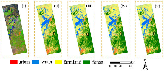
Figure 8.
Classification results of different algorithms. (i) Sentinel-2A (11-8-3/SWIR-NIR-Green), (ii) RF, (iii) KNN, (iv) 1DCNN, (v) 1DCNN-MRF.
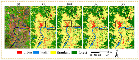
Figure 9.
Detailed comparison of the classification results of different algorithms. (i) Sentinel-2A (11-8-3/SWIR-NIR-Green), (ii) RF, (iii) KNN, (iv) 1DCNN, (v) 1DCNN-MRF.
5. Discussion
5.1. DpRVIm
Many existing satellites provide dual-pol mode data, which contained less information compared to full-pol mode. In the case of relatively few available features, many researchers have enriched the features by extracting vegetation indexes. Currently, the existing vegetation indexes are widely used in research areas such as crop monitoring [35], forest monitoring [34], and soil moisture inversion [33]. To study the efficiency of the DpRVIm in LCC, the DpRVI [31] and RVI [57] were chosen for the comparative experimental analysis. In this research, the degree of separability of most different land types was low, except water, when using only single temporal backscatter coefficient features. After introducing the classical index, the DpRVI, the accuracy slightly improved for all land cover types compared to introducing the RVI or using only the backscatter coefficient.
In this paper, the DpRVIm was proposed based on the DpRVI, polarization entropy, and DEM. DpRVIm improved the situation in which forest and farmland are prone to misclassification and omission. It can be reasoned that the polarized entropy will characterize the degree of randomness of the different ground objects, and the DEM is an important feature factor, which had a significant impact on the distribution of natural vegetation, farmland, urban, and water. In general, although both the DpRVI and the proposed DpRVIm can improve the accuracy of LCC, the introduction of the proposed DpRVIm had higher accuracy. After analyzing the reasons, both of them were presented with polarization decomposition, which indicated polarization decomposition is advantageous in LCC. This also showed that the combination of the polarization entropy and DEM was helpful to enhance the separability of different ground land objects.
Moreover, the study was limited to single temporal data. In fact, different vegetation has different phenological periods. Therefore, with the multi-temporal data, the vegetation index and scattering coefficients had a more complete response to the feature changes in different periods, which indicated that the DpRVIm also had advantages in multi-temporal data classification.
5.2. Comparative Analysis of Different Classification Methods
Machine learning algorithms have a crucial impact on the results of classification [60]. The classical pixel-based machine learning algorithms, RF, KNN, etc., have a wide range of applications in LCC [61,62]. In order to show the results of the proposed 1DCNN-MRF, the classical machine learning algorithms, RF, KNN, and the 1DCNN, were selected for comparative analysis. The results of the experiments showed that the effect of the 1DCNN-MRF was better than that of the machine learning methods, RF, KNN, and the 1DCNN. The classification results obtained by RF, KNN, and the 1DCNN all showed scattered fragmentation. This was because these methods are pixel-based classification, which can be affected easily by the speckle noise in SAR images. The 1DCNN-MRF alleviated the common problems caused by speckle noise and showed good classification accuracy for almost each type of land cover. For example, the omission error of the farmland increased slightly, and the commission error decreased accordingly. This was because the MRF algorithm was affected by the neighboring ground label field, while some of the farmland in the study area was fragmented, and the data had a low resolution of 10 m, leading to an increase in the omission error of more than 1%; however, the misclassification error phenomenon was reduced effectively at the same time. The MRF took into account the spatial information by calculating the energy of the feature field and label field to obtain the total energy. When the total energy was larger, this meant that the type of pixel was less likely to be the same as the neighboring ones, and the pixel that was misclassified would be corrected by the principle of the minimum energy.
The pixel-level classification methods play an important role in LCC [63], and the coherent speckle noise of SAR is also a problem that cannot be ignored [64]. The current research is more concerned with optimizing the network structure for SAR image despeckling [65,66]. The proposed method, the 1DCNN-MRF, provided another idea of noise immunity, which can retain the existing network structure and combine the characteristics of the MRF to achieve the corresponding noise immunity effect. Therefore, the idea of combining the MRF and 1DCNN can be extended to other pixel-based classification methods to improve the ability of the method against coherent speckle noise.
However, there were still some shortcomings in the 1DCNN-MRF designed in this paper. The method only considered the correlation between neighboring pixels, while the relationship between pixels was not limited to neighboring pixels, and the global spatial information was not sufficiently considered. The subsequent attempts will combine the super-pixel idea, which can effectively use the information such as the size of regional objects and reduce the interference of speckle noise with the classification results. The 1DCNN and MRF methods involve several parameter adjustments, and the choice of these parameters may have a large impact on the performance of the model, which may consume a large amount of time and computational resources. Subsequently, we will try to determine the parameters adaptively by combining the prior knowledge of the land type distribution.
6. Conclusions
In this study, a vegetation index, the DpRVIm, based on polarization information and the DEM was proposed, and a 1DCNN-MRF method with good noise robustness was designed. Furthermore, the role of some existing indexes in the dual-pol data, such as the RVI and DpRVI, were verified. Specifically, firstly, the backscatter coefficient, RVI, DpRVI, and DpRVIm were extracted from the dual-pol data. Next, the optimal feature combination was selected by numerical distribution analysis, J-M distance analysis, and the 1DCNN algorithm. Finally, the 1DCNN-MRF method was designed to combine the advantages of the 1DCNN and MRF, with the optimal feature combination as the input.
One of the findings was that the DpRVI based on polarization decomposition was not only suitable for soil moisture inversion and crop growth monitoring, but also for enhancing the separability of ground objects in LCC. Compared with the classic DpRVI, the DpRVIm proposed in the study had better separability of farmland and forest after combining the polarization entropy and DEM, which made it more adaptable in areas influenced by topography. This experimental result showed that the DpRVI and the proposed DpRVIm obtained good effects in HH-HV polarization mode.
Furthermore, we proposed the 1DCNN-MRF model, which had greater potential for SAR LCC. In order to estimate the effectiveness of the 1DCNN-MRF, RF, KNN, and the 1DCNN were investigated with SAR data. The results showed that the 1DCNN-MRF method using the + + DpRVIm combination achieved the highest classification accuracy with an OA value of 81.76%, which proved the LCC ability of the 1DCNN-MRF based on SAR data.
This can also indicate that the MRF algorithm can be combined with other pixel-based classification algorithms to obtain a better land cover product in SAR LCC, which is liable to be affected by coherent speckle noise.
Author Contributions
Conceptualization, M.M., Y.H. and N.L.; data curation, L.W. and Z.G.; investigation, M.M., Y.H. and N.L.; methodology, M.M., Y.H. and L.W.; supervision, M.M., Y.H., X.S. and Z.G.; writing—original draft, Y.H. and L.W.; writing—review and editing, M.M., Y.H., W.Z., Z.H. and N.L. All authors have read and agreed to the published version of the manuscript.
Funding
This work was supported by the National Natural Science Foundation of China (42101386), the Plan of Science and Technology of Henan Province (232102211043, 222102110439), the Key Laboratory of Natural Resources Monitoring and Regulation in Southern Hilly Region, the Ministry of Natural Resources of the People’s Republic of China (NRMSSHR2022Z01), the National Undergraduate Training Program for Innovation and Entrepreneurship (202210475111), and the Key Laboratory of Land Satellite Remote Sensing Application, the Ministry of Natural Resources of the People’s Republic of China (KLSMNR-202302).
Data Availability Statement
All data and models presented in this study are available.
Conflicts of Interest
The authors declare no conflict of interest.
References
- Zhao, J.; Wang, L.; Yang, H.; Wu, P.; Wang, B.; Pan, C.; Wu, Y. A land cover classification method for high-resolution remote sensing images based on NDVI deep learning fusion network. Remote Sens. 2022, 14, 5455. [Google Scholar] [CrossRef]
- Lin, X.; Xu, M.; Cao, C.; Singh, R.P.; Chen, W.; Ju, H. Land-use/land-cover changes and their influence on the ecosystem in Chengdu City, China during the period of 1992–2018. Sustainability 2018, 10, 3580. [Google Scholar] [CrossRef]
- Liu, S.; Qi, Z.; Li, X.; Yeh, A.G.-O. Integration of convolutional neural networks and object-based post-classification refinement for land use and land cover mapping with optical and SAR data. Remote Sens. 2019, 11, 690. [Google Scholar] [CrossRef]
- Kpienbaareh, D.; Sun, X.; Wang, J.; Luginaah, I.; Bezner Kerr, R.; Lupafya, E.; Dakishoni, L. Crop type and land cover mapping in northern Malawi using the integration of sentinel-1, sentinel-2, and planetscope satellite data. Remote Sens. 2021, 13, 700. [Google Scholar] [CrossRef]
- Zhang, C.; Sargent, I.; Pan, X.; Li, H.; Gardiner, A.; Hare, J.; Atkinson, P.M. Joint Deep Learning for land cover and land use classification. Remote Sens. Environ. 2019, 221, 173–187. [Google Scholar] [CrossRef]
- Kussul, N.; Lavreniuk, M.; Skakun, S.; Shelestov, A. Deep learning classification of land cover and crop types using remote sensing data. IEEE Geosci. Remote Sens. Lett. 2017, 14, 778–782. [Google Scholar] [CrossRef]
- Jia, W.; Pei, T.; Lei, K. Research on land use planning based on multisource remote sensing data. Comput. Intell. Neurosci. 2022, 2022, 5851768. [Google Scholar] [CrossRef]
- Xia, B.; Kong, F.; Zhou, J.; Wu, X.; Xie, Q. Land resource use classification using deep learning in ecological remote sensing images. Comput. Intell. Neurosci. 2022, 2022, 7179477. [Google Scholar] [CrossRef]
- Gao, W.; Yang, J.; Ma, W. Land cover classification for polarimetric SAR images based on mixture models. Remote Sens. 2014, 6, 3770–3790. [Google Scholar] [CrossRef]
- Wang, H.; Xing, C.; Yin, J.; Yang, J. Land cover classification for polarimetric SAR images based on vision transformer. Remote Sens. 2022, 14, 4656. [Google Scholar] [CrossRef]
- Sukawattanavijit, C.; Chen, J.; Zhang, H. GA-SVM algorithm for improving land-cover classification using SAR and optical remote sensing data. IEEE Geosci. Remote Sens. Lett. 2017, 14, 284–288. [Google Scholar] [CrossRef]
- Habibi, M.; Sahebi, M.R.; Maghsoudi, Y.; Ghayourmanesh, S. Classification of polarimetric SAR data based on object-based multiple classifiers for urban land-cover. J. Indian Soc. Remote Sens. 2016, 44, 855–863. [Google Scholar] [CrossRef]
- Arisoy, S.; Kayabol, K. Mixture-based superpixel segmentation and classification of SAR images. IEEE Geosci. Remote Sens. Lett. 2016, 13, 1721–1725. [Google Scholar] [CrossRef]
- Ahishali, M.; Kiranyaz, S.; Ince, T.; Gabbouj, M. Dual and single polarized SAR image classification using compact convolutional neural networks. Remote Sens. 2019, 11, 1340. [Google Scholar] [CrossRef]
- Singh, M.K.; Singha, N.S. A relaxed Gaussian mixture model framework for terrain classification based on distinct range datasets. Remote Sens. Lett. 2022, 13, 470–479. [Google Scholar] [CrossRef]
- Ulaby, F. Radar response to vegetation. IEEE Trans. Antennas Propag. 1975, 23, 36–45. [Google Scholar] [CrossRef]
- Wiseman, G.; McNairn, H.; Homayouni, S.; Shang, J. RADARSAT-2 polarimetric SAR response to crop biomass for agricultural production monitoring. IEEE J. Sel. Top. Appl. Earth Obs. Remote Sens. 2014, 7, 4461–4471. [Google Scholar] [CrossRef]
- Ohki, M.; Shimada, M. Large-area land use and land cover classification with quad, compact, and dual polarization SAR data by PALSAR-2. IEEE Trans. Geosci. Remote Sens. 2018, 56, 5550–5557. [Google Scholar] [CrossRef]
- Ghasemi, N.; Sahebi, M.R.; Mohammadzadeh, A. A review on biomass estimation methods using synthetic aperture radar data. Int. J. Geomat. Geosci. 2011, 1, 776–788. [Google Scholar]
- Lee, J.S.; Ainsworth, T.L.; Wang, Y. Polarization orientation angle and polarimetric SAR scattering characteristics of steep terrain. IEEE Trans. Geosci. Remote Sens. 2018, 56, 7272–7281. [Google Scholar] [CrossRef]
- Lee, J.S.; Ainsworth, T.L. The effect of orientation angle compensation on coherency matrix and polarimetric target decompositions. IEEE Trans. Geosci. Remote Sens. 2010, 49, 53–64. [Google Scholar] [CrossRef]
- Inglada, J.; Vincent, A.; Arias, M.; Marais-Sicre, C. Improved early crop type identification by joint use of high temporal resolution SAR and optical image time series. Remote Sens. 2016, 8, 362. [Google Scholar] [CrossRef]
- Notarnicola, C.; Angiulli, M.; Posa, F. Use of radar and optical remotely sensed data for soil moisture retrieval over vegetated areas. IEEE Trans. Geosci. Remote Sens. 2006, 44, 925–935. [Google Scholar] [CrossRef]
- Periasamy, S. Significance of dual polarimetric synthetic aperture radar in biomass retrieval: An attempt on Sentinel-1. Remote Sens. Environ. 2018, 217, 537–549. [Google Scholar] [CrossRef]
- Bhogapurapu, N.; Dey, S.; Mandal, D.; Bhattacharya, A.; Karthikeyan, L.; McNairn, H.; Rao, Y. Soil moisture retrieval over croplands using dual-pol L-band GRD SAR data. Remote Sens. Environ. 2022, 271, 112900. [Google Scholar] [CrossRef]
- Chang, J.G.; Shoshany, M.; Oh, Y. Polarimetric radar vegetation index for biomass estimation in desert fringe ecosystems. IEEE Trans. Geosci. Remote Sens. 2018, 56, 7102–7108. [Google Scholar] [CrossRef]
- Yamaguchi, Y.; Moriyama, T.; Ishido, M.; Yamada, H. Four-component scattering model for polarimetric SAR image decomposition. IEEE Trans. Geosci. Remote Sens. 2005, 43, 1699–1706. [Google Scholar] [CrossRef]
- Singh, G.; Yamaguchi, Y. Model-based six-component scattering matrix power decomposition. IEEE Trans. Geosci. Remote Sens. 2018, 56, 5687–5704. [Google Scholar] [CrossRef]
- Ratha, D.; Mandal, D.; Kumar, V.; Mcnairn, H.; Bhattacharya, A.; Frery, A.C. A generalized volume scattering model-based vegetation index from polarimetric SAR data. IEEE Geosci. Remote Sens. Lett. 2019, 16, 1791–1795. [Google Scholar] [CrossRef]
- Ratha, D.; De, S.; Celik, T.; Bhattacharya, A. Change detection in polarimetric SAR images using a geodesic distance between scattering mechanisms. IEEE Geosci. Remote Sens. Lett. 2017, 14, 1066–1070. [Google Scholar] [CrossRef]
- Mandal, D.; Kumar, V.; Ratha, D.; Dey, S.; Bhattacharya, A.; Lopez-Sanchez, J.M.; McNairn, H.; Rao, Y.S. Dual polarimetric radar vegetation index for crop growth monitoring using sentinel-1 SAR data. Remote Sens. Environ. 2020, 247, 111954. [Google Scholar] [CrossRef]
- Bayaraa, B.; Hirano, A.; Purevtseren, M.; Vandansambuu, B.; Damdin, B.; Natsagdorj, E. Applicability of different vegetation indices for pasture biomass estimation in the north-central region of Mongolia. Geocarto Int. 2021, 37, 7415–7430. [Google Scholar] [CrossRef]
- Shilpa, K.; Raju, C.S.; Mandal, D.; Rao, Y.S.; Shetty, A. Soil moisture retrieval over crop fields from multi-polarization SAR data. J. Indian Soc. Remote Sens. 2023, 51, 949–962. [Google Scholar] [CrossRef]
- Tanase, M.; de la Riva, J.; Santoro, M.; Pérez-Cabello, F.; Kasischke, E. Sensitivity of SAR data to post-fire forest regrowth in Mediterranean and boreal forests. Remote Sens. Environ. 2011, 115, 2075–2085. [Google Scholar] [CrossRef]
- Villarroya-Carpio, A.; Lopez-Sanchez, J.M. Multi-annual evaluation of time series of sentinel-1 interferometric coherence as a tool for crop monitoring. Sensors 2023, 23, 1833. [Google Scholar] [CrossRef]
- Shimizu, K.; Murakami, W.; Furuichi, T.; Estoque, R.C. Mapping land use/land cover changes and forest disturbances in vietnam using a landsat temporal segmentation algorithm. Remote Sens. 2023, 15, 851. [Google Scholar] [CrossRef]
- Tang, R.; Pu, F.; Yang, R.; Xu, Z.; Xu, X. Multi-domain fusion graph network for semi-supervised PolSAR image classification. Remote Sens. 2022, 15, 160. [Google Scholar] [CrossRef]
- Jin, Y.; Guan, X.; Ge, Y.; Jia, Y.; Li, W. Improved spatiotemporal information fusion approach based on bayesian decision theory for land cover classification. Remote Sens. 2022, 14, 6003. [Google Scholar] [CrossRef]
- Magalhães, I.A.L.; de Carvalho Júnior, O.A.; de Carvalho, O.L.F.; de Albuquerque, A.O.; Hermuche, P.M.; Merino, É.R.; Gomes, R.A.T.; Guimarães, R.F. Comparing machine and deep learning methods for the phenology-based classification of land cover types in the amazon biome using sentinel-1 time series. Remote Sens. 2022, 14, 4858. [Google Scholar] [CrossRef]
- Chakhar, A.; Hernández-López, D.; Ballesteros, R.; Moreno, M.A. Improving the accuracy of multiple algorithms for crop classification by integrating sentinel-1 observations with sentinel-2 data. Remote Sens. 2021, 13, 243. [Google Scholar] [CrossRef]
- Dobrinić, D.; Gašparović, M.; Medak, D. Sentinel-1 and 2 time-series for vegetation mapping using random forest classification: A case study of Northern Croatia. Remote Sens. 2021, 13, 2321. [Google Scholar] [CrossRef]
- Yuan, H.; Van Der Wiele, C.F.; Khorram, S. An automated artificial neural network system for land use/land cover classification from landsat TM imagery. Remote Sens. 2009, 1, 243–265. [Google Scholar] [CrossRef]
- Dahhani, S.; Raji, M.; Hakdaoui, M.; Lhissou, R. Land cover mapping using sentinel-1 time-series data and machine-learning classifiers in agricultural sub-saharan landscape. Remote Sens. 2022, 15, 65. [Google Scholar] [CrossRef]
- Solórzano, J.V.; Mas, J.F.; Gao, Y.; Gallardo-Cruz, J.A. Land use land cover classification with U-net: Advantages of combining sentinel-1 and sentinel-2 imagery. Remote Sens. 2021, 13, 3600. [Google Scholar] [CrossRef]
- He, C.; He, B.; Tu, M.; Wang, Y.; Qu, T.; Wang, D.; Liao, M. Fully convolutional networks and a manifold graph embedding-based algorithm for polsar image classification. Remote Sens. 2020, 12, 1467. [Google Scholar] [CrossRef]
- Mei, S.; Ji, J.; Hou, J.; Li, X.; Du, Q. Learning sensor-specific spatial-spectral features of hyperspectral images via convolutional neural networks. IEEE Trans. Geosci. Remote Sens. 2017, 55, 4520–4533. [Google Scholar] [CrossRef]
- Joshi, R.; Garg, R.D. Pre-processing of TerraSAR-X data for speckle removal: An approach for performance evaluation. J. Indian Soc. Remote Sens. 2012, 40, 371–377. [Google Scholar] [CrossRef]
- Hasan, S.F.; Shareef, M.A.; Hassan, N.D. Speckle filtering impact on land use/land cover classification area using the combination of Sentinel-1A and Sentinel-2B (a case study of Kirkuk city, Iraq). Arab. J. Geosci. 2021, 14, 276. [Google Scholar] [CrossRef]
- Wang, C.; Jiang, W.; Deng, Y.; Ling, Z.; Deng, Y. Long time series water extent analysis for SDG 6.6. 1 based on the GEE platform: A case study of Dongting Lake. IEEE J. Sel. Top. Appl. Earth Obs. Remote Sens. 2021, 15, 490–503. [Google Scholar] [CrossRef]
- Jiang, W.; Hou, P.; Zhu, X.; Cao, G.; Liu, X.; Cao, R. Analysis of vegetation response to rainfall with satellite images in Dongting Lake. J. Geogr. Sci. 2011, 21, 135–149. [Google Scholar] [CrossRef]
- Liu, D. PIE 6.0 remote sensing product system and application services. Satell. Appl. 2020, 5, 15–21. [Google Scholar]
- NASA. The Shuttle Radar Topography Mission (SRTM) Collection User Guide. Available online: https://lpdaac.usgs.gov/documents/179/SRTM_User_Guide_V3.pdf (accessed on 13 September 2020).
- Bai, Y.; Sun, X.; Ji, Y.; Huang, J.; Fu, W.; Shi, H. Bibliometric and visualized analysis of deep learning in remote sensing. Int. J. Remote Sens. 2022, 43, 5534–5571. [Google Scholar] [CrossRef]
- Zhou, Y.; Luo, J.; Feng, L.; Yang, Y.; Chen, Y.; Wu, W. Long-short-term-memory-based crop classification using high-resolution optical images and multi-temporal SAR data. GISci Remote Sens. 2019, 56, 1170–1191. [Google Scholar] [CrossRef]
- Van Den Broek, A.C.; Smith, A.J.E.; Toet, A. Land use classification of polarimetric SAR data by visual interpretation and comparison with an automatic procedure. Int. J. Remote Sens. 2004, 25, 3573–3591. [Google Scholar] [CrossRef]
- Kim, K.; Jung, H.C.; Choi, J.-K.; Ryu, J.-H. Statistical analysis for tidal flat classification and topography using multitemporal SAR backscattering coefficients. Remote Sens. 2021, 13, 5169. [Google Scholar] [CrossRef]
- Trudel, M.; Charbonneau, F.; Leconte, R. Using RADARSAT-2 polarimetric and ENVISAT-ASAR dual-polarization data for estimating soil moisture over agricultural fields. Can. J. Remote Sens. 2012, 38, 514–527. [Google Scholar]
- Ito, Y.; Omatu, S. Polarimetric SAR data classification using competitive neural networks. Int. J. Remote Sens. 1998, 19, 2665–2684. [Google Scholar] [CrossRef]
- Dabboor, M.; Howell, S.; Shokr, M.; Yackel, J. The Jeffries–Matusita distance for the case of complex Wishart distribution as a separability criterion for fully polarimetric SAR data. Int. J. Remote Sens. 2014, 35, 6859–6873. [Google Scholar]
- Imangholiloo, M.; Rasinmäki, J.; Rauste, Y.; Holopainen, M. Utilizing Sentinel-1A radar images for large-area land cover mapping with machine-learning methods. Can. J. Remote Sens. 2019, 45, 163–175. [Google Scholar] [CrossRef]
- Garg, R.; Kumar, A.; Prateek, M.; Pandey, K.; Kumar, S. Land cover classification of spaceborne multifrequency SAR and optical multispectral data using machine learning. Adv. Space Res. 2022, 69, 1726–1742. [Google Scholar] [CrossRef]
- Elmahdy, S.I.; Mohamed, M.M. Regional mapping and monitoring land use/land cover changes: A modified approach using an ensemble machine learning and multitemporal Landsat data. Geocarto Int. 2023, 38, 2184500. [Google Scholar] [CrossRef]
- Muthukumarasamy, I.; Shanmugam, R.S.; Kolanuvada, S.R. SAR polarimetric decomposition with ALOS PALSAR-1 for agricultural land and other land use/cover classification: Case study in Rajasthan, India. Environ. Earth Sci. 2017, 76, 455. [Google Scholar] [CrossRef]
- Guan, D.; Xiang, D.; Tang, X.; Wang, L.; Kuang, G. Covariance of textural features: A new feature descriptor for SAR image classification. IEEE J. Sel. Top. Appl. Earth Obs. Remote Sens. 2019, 12, 3932–3942. [Google Scholar] [CrossRef]
- Wen, Z.; He, Y.; Yao, S.; Yang, W.; Zhang, L. A self-attention multi-scale convolutional neural network method for SAR image despeckling. Int. J. Remote Sens. 2023, 44, 902–923. [Google Scholar] [CrossRef]
- Zhang, Q.; Yuan, Q.; Li, J.; Yang, Z.; Ma, X. Learning a dilated residual network for SAR image despeckling. Remote Sens. 2018, 10, 196. [Google Scholar] [CrossRef]


Disclaimer/Publisher’s Note: The statements, opinions and data contained in all publications are solely those of the individual author(s) and contributor(s) and not of MDPI and/or the editor(s). MDPI and/or the editor(s) disclaim responsibility for any injury to people or property resulting from any ideas, methods, instructions or products referred to in the content. |
© 2023 by the authors. Licensee MDPI, Basel, Switzerland. This article is an open access article distributed under the terms and conditions of the Creative Commons Attribution (CC BY) license (https://creativecommons.org/licenses/by/4.0/).