
Remote Sensing of Geomorphodiversity Linked to Biodiversity—Part III: Traits, Processes and Remote Sensing Characteristics

 , ,
, ,  , , , , ,
  ,
,  , , , , ,
  , , , , ,
  ,
,  ,
,  , , and
Abstract
:1. Introduction
- To describe the five characteristics of geomorphodiversity;
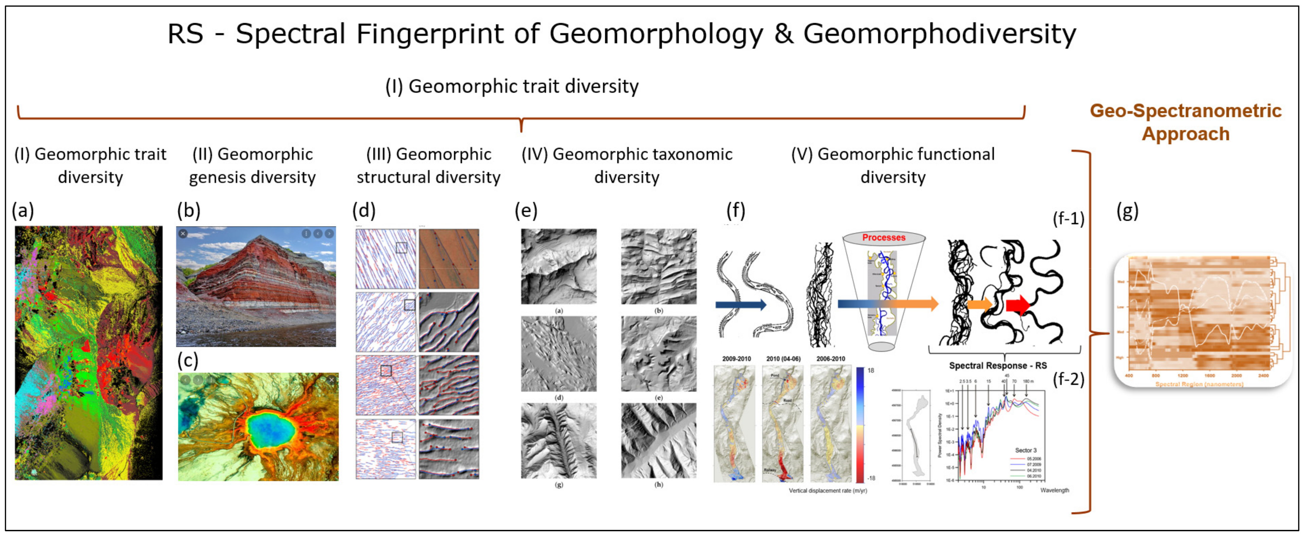
- To extensively discuss and explain the monitoring of the five geomorphodiversity features, based on RS approaches, which are geomorphic genesis diversity, geomorphic trait diversity, geomorphic structural diversity, geomorphic taxonomic diversity, and geomorphic functional diversity;
- To explain the approach when monitoring geomorphic traits and trait variations using RS technologies, and the advantages and constraints of RS technologies for monitoring the five characteristics of geomorphodiversity;
- To explore the need to consider the characteristics and the spatial-temporal distribution of geomorphic traits for successful RS-based monitoring;
- To discuss methods for distinguishing and classifying the five features of geomorphodiversity using RS;
- To discuss RS-based methods for monitoring geomorphodiversity in regimes with changing land-use intensity;
- To elucidate new approaches for monitoring geomorphodiversity, using multi-mission RS approaches and the ecosystem integrity approach;
- To highlight the importance of digitization processes and the use of data science approaches for geomorphological research in the 21st century.
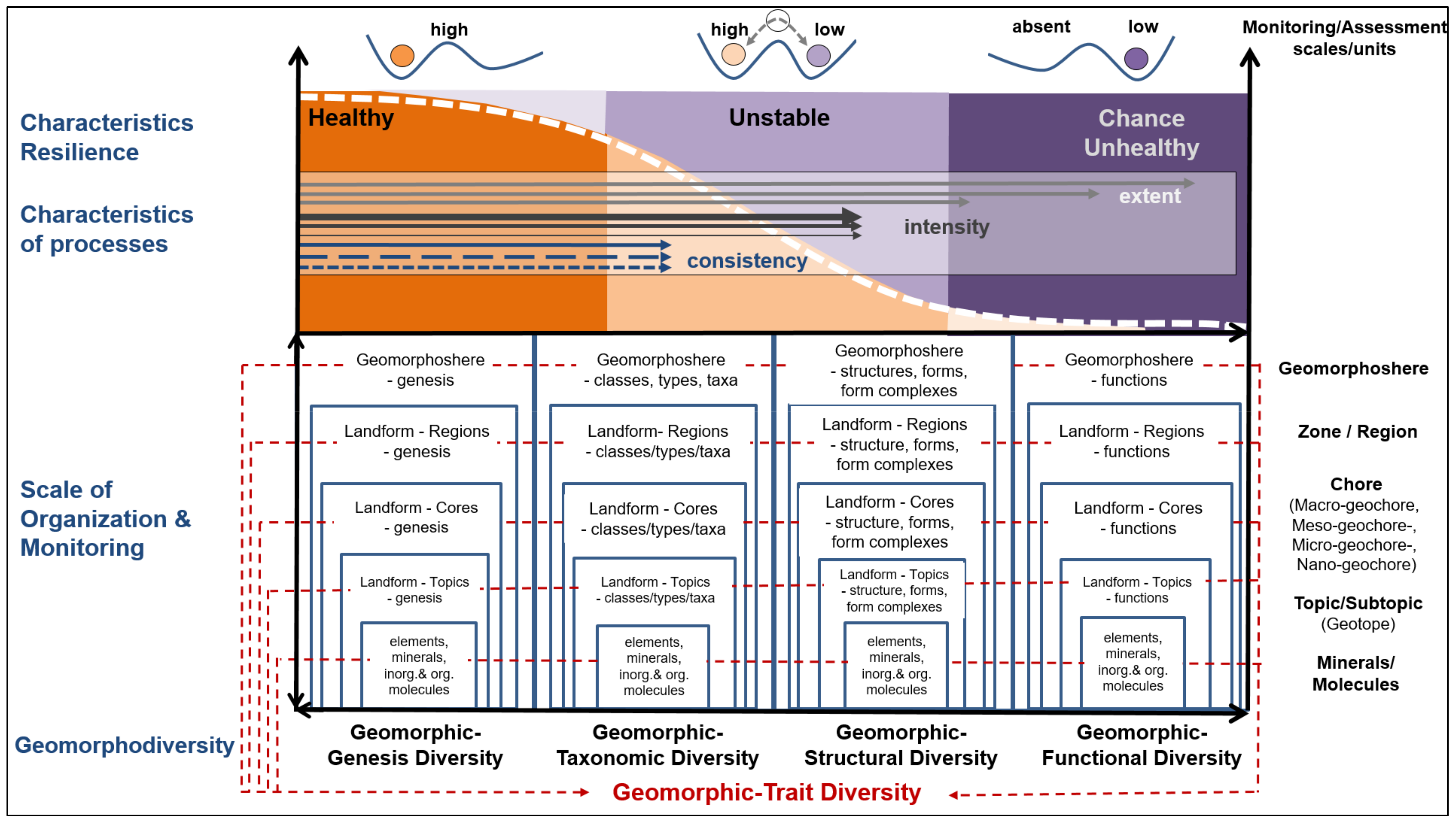
2. Characteristics of Geomorphodiversity
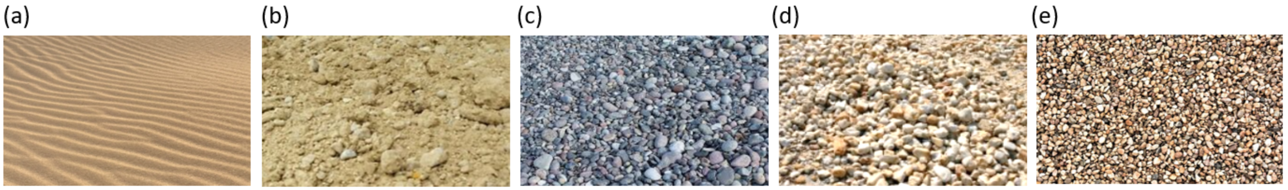
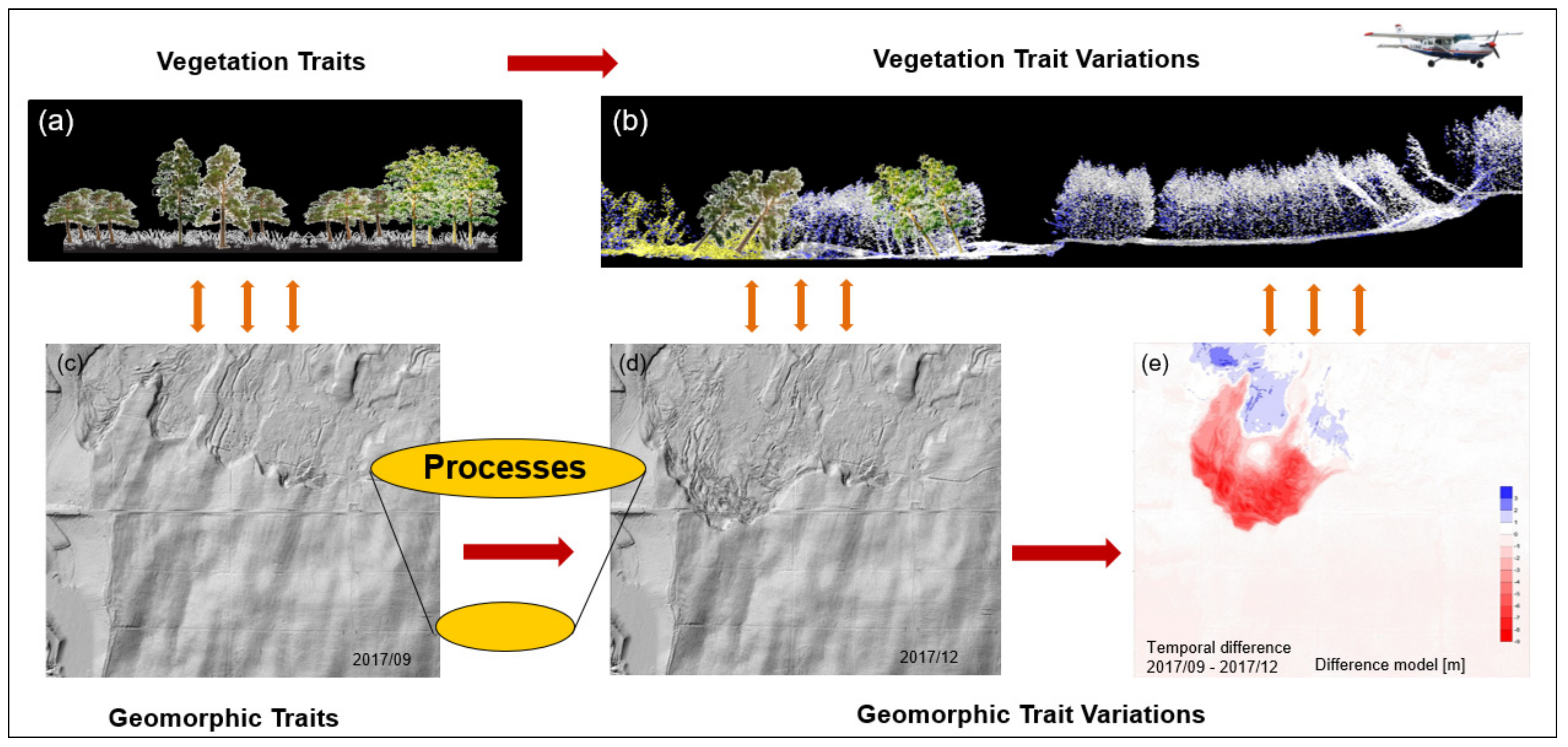
- Geomorphic trait diversity, which represents the diversity of mineralogical, bio-/geochemical, bio-/geo-optical, chemical, physical, morphological, structural, textural, or functional characteristics of geomorphic components that affect, interact with, or are influenced by geomorphic genesis diversity, geomorphic taxonomic diversity, geomorphic structural diversity, and geomorphic functional diversity.
- Geomorphic genesis diversity represents the diversity of the length of evolutionary pathways, linked to a given set of geomorphic traits, taxa, structures, and functions. Therefore, sets of geomorphic traits, taxa, structures, and functions are identified that maximize the accumulation of geomorphic-functional diversity.
- Geomorphic structural diversity, which is the diversity of composition and configuration of 2D to 4D geomorphic structural traits.
- Geomorphic taxonomic diversity, which stands for the diversity of geomorphic components that differ from a taxonomic perspective.
- Geomorphic functional diversity, which is the diversity of geomorphic functions and processes, as well as their intra- and interspecific interactions.
3. Monitoring Geomorphodiversity and Its Variability
3.1. In Situ Approaches—Field-Mapping Techniques
- In situ technologies are the most direct method for collecting the actual geological data required for calibrating and validating RS data, which are crucial for understanding, assessing and predicting geo-genesis and structural, taxonomic and functional geomorphodiversity;
- In situ methods enable high precision, timely measurements, are often weather-independent and offer continuous measurements with high temporal frequency;
- Time consumption, laboratory and technical expenditure is high;
- Intercalibrations have to be performed to achieve the comparability of different in situ sensor technologies;
- There are limitations to the spatial (grain or extent), directional and temporal resolution of in situ measuring devices; therefore, there are limited possibilities for investigating spatial-temporal as well as directional scale effects;
- There are limitations to investigating the interactions of geomorphological processes on a regional, continental and global scale.
3.2. RS Approaches
3.3. Constraints for Monitoring Geomorphodiversity with RS
3.3.1. Characteristics and the Spatial-Temporal Distribution of Geomorphic Traits
3.3.2. Characteristics of Geomorphic Processes and Their Drivers
3.3.3. Sensor Properties and Platforms to Monitor Geomorphodiversity
3.3.4. Summary of Constraints
- The characteristics of the combinations of geomorphic processes (i.e., the scope, length, intensity, consistency, dominance, and overlay) that lead to the formation of characteristic geomorphic traits, geo-genesis, taxonomic, structural, and functional diversity.
- The characteristics, composition, and configuration, such as the shape, density or distribution of the geomorphic traits and trait variations in space and over time.
- The radiometric, spectral, spatial, and temporal resolution of the RS sensors are crucial for the successful detection and monitoring of the five features of geomorphodiversity.
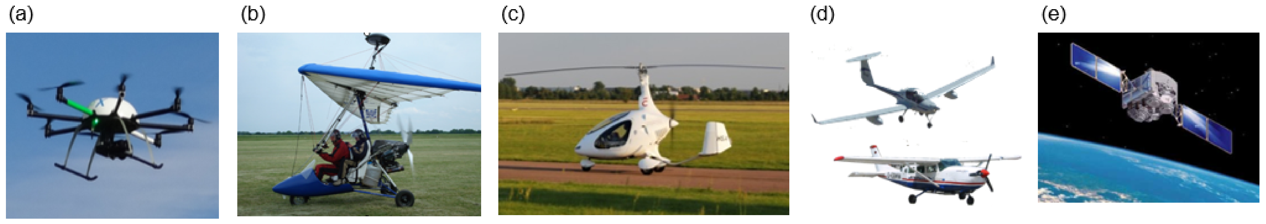
- The choice of RS platform (close-range, air- or spaceborne) influences the spatial and temporal resolution and, ultimately, the recordability and precision of the RS sensor properties of the geomorphic traits.
- The choice of the classification method (spectral-based pixel classification or spectral-based geographic object-based image analysis (GEOBIA) [95]), and how well the applied classification algorithm and its assumptions fit the RS data and the spectral traits of geomorphology.
- Sensors with different sensing properties should be combined to detect different geomorphic traits and trait variations simultaneously.
- A multi-variate and multi-temporal implementation of RS sensors, such as multispectral, hyperspectral, LiDAR, RADAR, microwave radiometer, and thermal infrared (TIR) sensors, increase not only the number but also the characteristics and diversity of geomorphic traits and trait variations that can be recorded.
- Geomorphological features/traits should be captured with a combination of sensors to combine different RS advantages (a multi-sensor and multi-temporal RS approach) and to compensate for and/or complement the technological limitations of sensors. For example, synthetic aperture radar (SAR) data for 5 m2 contains mixed information about geomorphic traits, with the advantages of other sensor technologies (e.g., 25 points/m2 of LiDAR data to record DEM and its changes).
4. Monitoring Five Characteristics of Geomorphodiversity Using RS
4.1. Geomorphic Trait Diversity and Its Changes Using RS
4.2. Geomorphic Genesis Diversity Using RS
4.3. Geomorphic Structural Diversity Using RS
4.4. Geomorphic Taxonomic Diversity Using RS
4.5. Geomorphic Functional Diversity Using RS
5. Monitoring Geomorphodiversity in Regimes with Changing Land-Use Intensity
6. Methods for Discriminating and Classifying the Five Characteristics of Geomorphodiversity
- The different geomorphic characteristics differ in their geomorphic traits, such as geochemical or mineralogical properties (color, grain size, aggregate state, geochemical characteristics, mineralogical composition, and configurations such as sand, clay, boulders, rock- and soil types) or water regimes.
- By their 2D–3D morphometric and structural properties, shapes such as horizontal and vertical structures, shape types, and shape groups differ from each other. Additional information, such as DEM-derived geomorphic variables including slope, aspect, indicators of roughness, relief shading, etc., can be used to improve discrimination performance [98].
- Likewise, the occurrence of specific lithological and soil characteristics resulting from evolutionary, climate, or anthropogenic drivers can be captured with RS data, which can improve discrimination performance.
- The geomorphometric delineation of landforms, such as fluvial landforms, i.e., floodplains and terraces, using objectively defined topographic and morphometric thresholds [124].
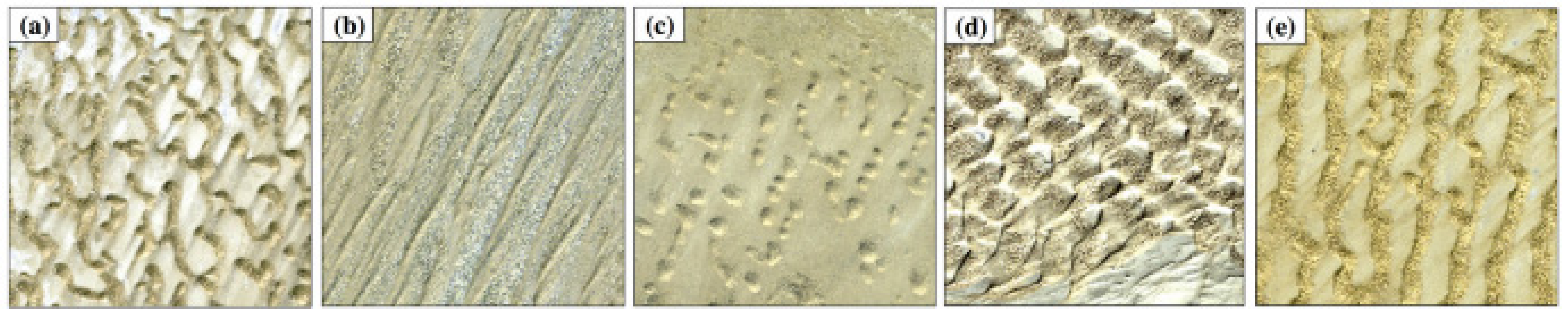
- When the characteristic variations of geomorphic traits occur within short time periods (days, years, or decades), e.g., gravimetric mass movements, aeolian formations, glacial movements, coastal formations, climate-induced permafrost changes, specific processes during volcanic eruptions, or aeolian processes through wind erosion, leading to the formation of specific dune classes [125].
- In addition to 2D–3D spatial patterns of geomorphology, trait characteristics and their distributions are also determined. From this, the trend of possible changes from evolutionary and anthropogenic patterns over time can be determined.
- Changes in shapes and patterns can be used to draw important conclusions about the characteristics and causes of anthropogenic influences, as anthropogenic geomorphic features are characterized by specific shapes and geochemical compositions (like, buildings, cities, roads, middens, terraces, megaliths, boundary walls, reservoirs, and river regulations) [17].
- The above factors are used to derive direct indicators.
- Specific 2-3D structures such as DEM/DSM and their shifts or disturbances are derived by using specific RS techniques, such as In-SAR, RADAR, LiDAR, GEDI-LiDAR [7].
- Different geomorphic characteristics lead to the development and distribution of characteristic bacteria, animal, and plant species (algae, weave, bacteria, symbiosis, animals, plants, and soil crusts), plant functional types (PFT, specific biological traits, growth characteristics, specific biochemical, structural and functional traits, or health status) of bacteria, plants or soil crusts as crucial bio-geomorphological indicators and proxies of different geomorphic characteristics, if specific geomorphic characteristics are present in the development of specific plant species, PFT, or in the context of geomorphodiversity as geo-plant fuctional types (G-PFT).
- Different geomorphic characteristics deviate in their geomorphic-specific ecological niches, and/or when various geomorphic characteristics lead to different geomorphic resource limitations for algae, weave, bacteria, specific symbiosis as well as specific animals, plants, and vegetation.
- The microclimate, outgassing, species composition changes, and chlorophyll or nitrogen increases (e.g., climate change or permafrost change) is supposed to change through anthropogenic influences.
- If the different characteristics of geomorphodiversity are not distinguished from each other by the aforementioned traits, multi-sensor RS data are used to improve the discrimination of geomorphic features and the recording of geomorphodiversity.
- When variations in geomorphic traits occur within short geomorphic periods (days, years, or decades), e.g., gravimetric mass movements, aeolian formations, glacier movements, coastal formations, climate-induced permafrost changes, volcano or aeolian processes through wind erosion, which lead to the formation of specific dune classes [125,128,129,130,131,132].
- However, where evolutionary periods are required to form shapes (tectonic, glacial, or fluvial formations), the use of the method of space-for-time substitution in geomorphology is useful [126]. In addition to the 2D–3D spatial patterns of geomorphology, trait characteristics, and the distribution of geomorphic traits, the trend of possible changes from evolutionary, as well as anthropogenic patterns over time, are determined.
- Furthermore, crucial conclusions about the characteristics and the origins of anthropogenic influence can be drawn from the shape change and, thus, the anthropogenic geomorphic forms (buildings, cities, roads, middens, terraces, megaliths, boundary walls, or reservoirs) can be discriminated using RS [17].
- Across the acquisition modes and along the electromagnetic spectrum, several techniques, from active electro-optical imaging (LiDAR) to active microwave observation techniques (RADAR, InSAR), are applicable to assess the different geomorphic diversities.
- In Table 1, the advantages and disadvantages of the different RS techniques are summarized for a direct comparison.
- A major conclusion from Table 1 is that only a combination of RS techniques covering large parts of the electromagnetic spectrum from visible light to microwaves may have the capability to sufficiently monitor and map the five geomorphic diversities.
- The multi-mission algorithm and analysis platform (MAAP) is listed as one option for geomorphodiversity monitoring. This online portal serves as a multi-mission data and algorithm cloud environment for sharing and processing data from different ESA and NASA missions, with a special focus on aboveground biomass (https://earthdata.nasa.gov/esds/maap, (accessed on 5 March 2022)).
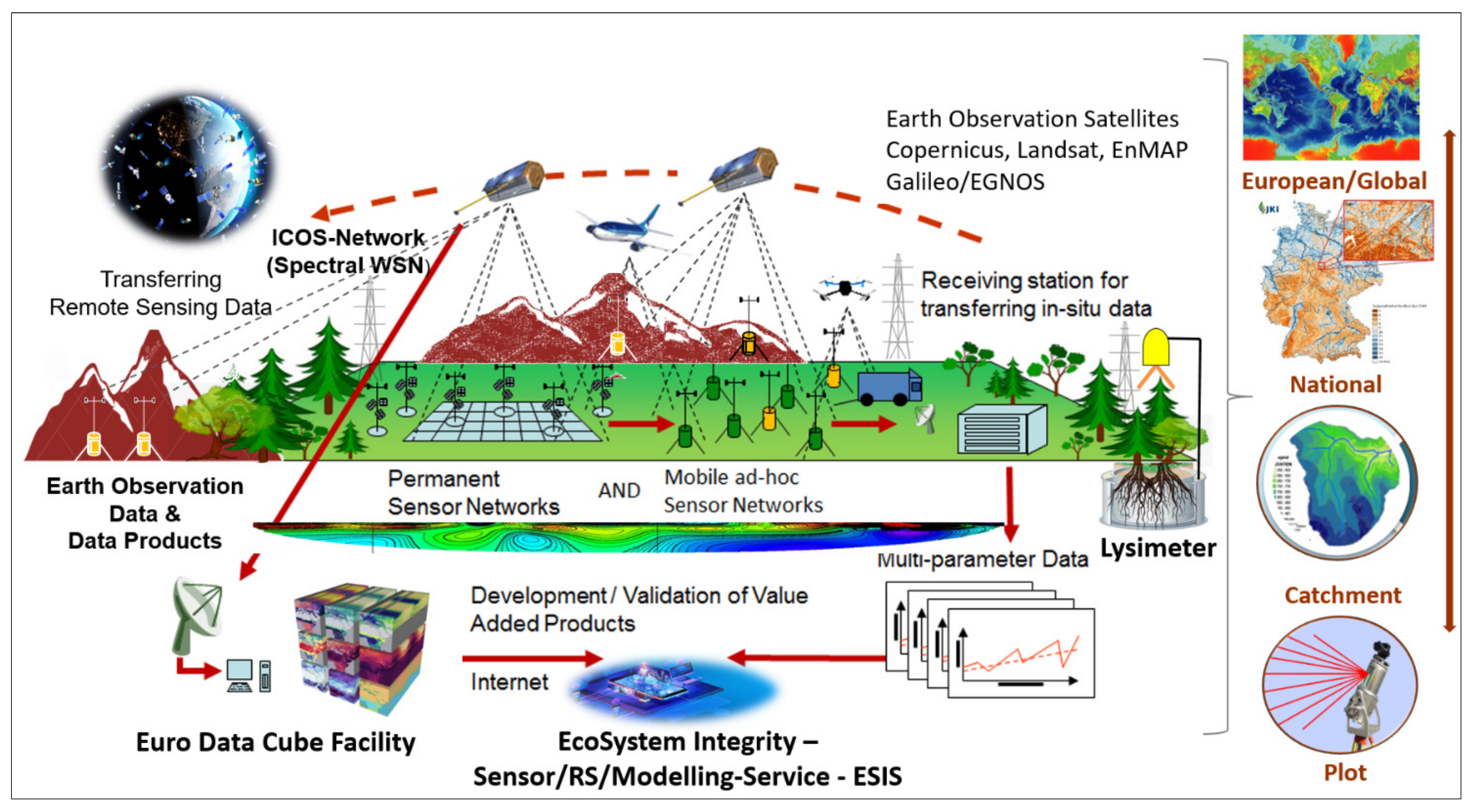
7. Ecosystem Integrity—In Situ/RS/Modeling Approach for Monitoring Geomorphodiversity
- An integration of in situ, close-range, air- and spaceborne RS monitoring technologies
- A link to the in situ monitoring approaches for the calibration and validation (cal/val) of RS data and the ability to support a data-driven modeling approach
- High-resolution remote sensing imagery [137]
- Modular coupling of spectral trait classification based on multi-sensor, multi-temporal RS data, and multi-mission algorithm and analysis platforms (like, MAAP)
- The identification and classification of geomorphic features, based on multi-algorithm and classification approaches, such as pixel-based classification, object-based image analysis (OBIA, [95]), the gray level co-occurrence matrix (GLCM [138]) modeling), geomorphic pattern recognition via artificial intelligence (AI), and machine learning [137]
- Direct links for recording spectral RS traits and data assimilation with process-modeling approaches (geomorphological models, morpho-hydrological models, biogeomorphological models, or vegetation models, such as the agent-based forest models).
8. Discussion of This Approach in the Context of the Existing Approaches of Geomorphodiversity
- (I)
- Approaches to the collection of indicators as a basis for the assessment of geomorphodiversity:
- (II)
- Approaches to geomorphodiversity and geodiversity assessment:
9. Conclusions of the Comparison
- So far, there is no comparable approach to capture the five characteristics of geomorphodiversity using only RS data and RS data products.
- Only the approach of Amatulli et al. [141], which derives 26 geomorphic indicators from RS, is partially comparable to the approach described here. Since spectral geomorphic traits exist on all spatial scales of geomorphology, indicators from the local and regional scales, up to the global scale, can be recorded by means of RS and used for assessment approaches.
- In terms of standardization and comparability across spatial scales, as described by Panizza [19] through the “extrinsic geodiversity” indicators, comparability across smaller spatial scales will be achieved, but this contradicts the approaches of [156,157,158] which state that each dimensional level is characterized by a specific geogenesis, structure, taxonomy, and functions and that the transition between spatial dimensions is defined by the criterion of homogeneity (geomorphic patch—a spatial unit that is homogeneous in its geomorphic traits).
- Geomorphic traits are defined by the thematic focus (genesis, structure, taxonomy, function, and process) and are subject to a spatial and temporal range of validity. Geomorphic traits exist on all spatio-temporal scales, but they are dimension-specific. In each spatial dimension, other geomorphic traits become more important. As the spatial dimension changes, the degree of generalization or abstraction level of the geomorphic traits changes. When applying the geomorphic trait/trait variation approach and the five characteristics of geomorphodiversity for the assessment and categorization of landscapes, the assessment approaches should be assessed according to the specific spatial dimension approaches (topic, choric, region, and zone).
- Standardized, comparable, repeatable indicators and monitoring and assessment procedures that are robustly applicable at all spatio-temporal scales of geomorphodiversity are needed [160].
10. Data Science to Monitor Geomorphodiversity
- To connect to environmental research infrastructures, such as: the environmental research infrastructures, ENVRIplus and ENVRIFair (big networks of in situ research infrastructures, linked to most of the domains of Earth systems sciences—the biosphere, the atmosphere, marine systems, and solid Earth) [161]; the European Observatory for research infrastructures and in situ Earth observation networks (ENEON); the Committee on Earth Observation Satellites (CEOS); the European Association of Remote Sensing Companies (EARSC); Copernicus, and others.
- To apply the EcoSystem Integrity RS/Modeling Service (ESIS) approach.
- To link in situ/field monitoring and IoT with close-range, air- and spaceborne RS platforms.
- To link different monitoring and modeling approaches with citizen science, etc.
- To use big data, open access, freely available data, open science clouds, distributed repositories, and the thematic exploitation platform (TEP).
- To integrate local, regional and global databases on geomorphology.
- To ensure the interoperability, standardization, and harmonization of data, monitoring, and decision-support systems. For example, with the help of metadata, using a standard open communication protocol, GoFAIR-Data (findable, accessible, interoperable, and re-usable) [169] and GoFAIR modeling approaches for scientific data management and stewardship related to metadata, data infrastructures (e.g., GAIA-X) and the International Data Spaces Association (IDSA), using the data cube approach with an n-D higher-dimensional array of values, including multi-petabyte data warehouses in clouds, the international data spaces (IDS) metadata broker, and the IDSA meta-model for geomorphology and RS time series.
- To integrate semantic data, semantic web/Web 4.0, ontology; linked open data (LOD) approaches based on the key enabling technologies (KETs) and knowledge organization systems (KOSs), and knowledge organization and management (KOMs), based on SNAP and SPAN ontologies [170], for the semantic interoperability of heterogeneous data [171].
- To implement complex data science modeling and analysis: AI, machine learning, deep learning, cloud computing, data mining, Hadoop, the Google Earth engine, hosting services, workflows, and others.
- To use data and RS data product cubes, the Euro Data Cube Facility, iCube, and open RS data cubes.
- To check the proof, trust, and uncertainties of in situ monitoring, RS, and data science uncertainties.
- To implement rapid warning systems for geohazards.
- To develop easy to handle software, tools for data managers, stakeholders, and politicians (visualization models, and dashboards).
11. Conclusions and Future Challenges for Monitoring Geomorphodiversity
- The presented trait approach presented here and the resulting indicators—spectral traits of geomorphology/geomorphodiversity—should be included in the future indicator list for the EGVs.
- Comparable to the approach and paper published by Diaz [172] (“The global spectrum of plant form and function”), “The global spectrum of geomorphology/geomorphodiversity” should be determined using the spectral geomorphic trait approach and its indicators.
- Geomorphic traits exist on all spatio-temporal scales, but they are dimension-specific. In each spatial dimension, other geomorphic traits become important. As the spatial dimension changes, the degree of generalization or abstraction level of the geomorphic traits changes. When using the geomorphic trait and trait variation approach and the five characteristics of geomorphodiversity for the assessment and categorization of landscapes, the assessment approaches should be used according to the specific spatial dimension approaches (topic, choric, region, or zone) [157].
Funding
Data Availability Statement
Acknowledgments
Conflicts of Interest
Appendix A

| Geomorphic Traits | Mission/Platform Sensor | References |
|---|---|---|
| Terrain and Surfaces/Traits | ||
| Geomorpho90 m (90 m/100 m/250 m) (slope, aspect, aspect cosine, aspect sine, eastness, northness, convergence, compound topographic index, stream power index, east-west first-order partial derivative, north-south first-order partial derivative, profile curvature, tangential curvature, east-west second-order partial derivative, north-south second-order partial derivative, second-order partial derivative, elevation standard deviation, terrain ruggedness index, roughness, vector ruggedness measure, topographic position index, maximum multiscale deviation, scale of the maximum multiscale deviation, maximum multiscale roughness, scale of the maximum multiscale roughness, geomorphon) | (26 geomorphometric variables derived from MERIT-DEM 3/R—corrected from the underlying Shuttle RADAR Topography Mission (SRTM3) and ALOS World 3D—30 m (AW3D30) DEMs) | [141] |
| Mountain types, relief types, relief classes | IKONOS OSA 3/M, DHM25 3/R, GTOPO30—DEM 3/R, LiDAR 2/L | [98,173,174] |
| Volcano types (volcanic full forms), volcanoes, lava flow fields, hydrothermal alteration, geothermal explorations, heat fluxes, volcanoes hazard monitoring, location, deformation | Doves-PlanetScop, Terra/Aqua MODIS 3/M, EO-1 ALI 3/M, Landsat-8 OLI 3/M/TIR, Terra ASTER 3/M/TIR, MSG SEVIRI 3/M/TIR, LiDAR 2/L | [109,175,176,177,178,179,180] |
| Mountain hazards, mass movement (rockfall probability, boulders, denudation, mass erosion, rock decelerations, rotation changes, slope stability, rock shapes, mineral distribution, geological material discrimination, particle shapes, patterns, structures, faults and fractures, holes, and depressions) mountain monitoring system | InSAR 3/R, SAR 3/R, LiDAR 2/L, Digital Orthophoto 1/RGB, HySPEC 2/HSP, AVIRIS 2/HSP | [96,181,182,183,184,185,186,187,188,189,190,191,192] |
| Landslide chances, landslide evolution | Digital Orthophoto 1/RGB | [193] |
| Above ground—chances, disturbances Opencast mining, sand mining and extraction, tipping, dumps | TanDEM-X 3/R, SRTM DEM 3/R, ALOS PALSAR 3/R, ERS-1 3/R, GeoEye GIS 3/M, WorldView-3 Imager 3/M, IKONOS OSA 3/M, Landsat-5 TM/-7 ETM ± 8 OLI 3/M/TIR, IRS-P6 LISS-III 3/M, High resolution satellite data of Google 3/M, LiDAR 2/L | [194,195,196,197,198,199,200] |
| Vegetation traits as proxy of the geochemical parameters | HyMAP 2/H | [201] |
| Below ground—chances, disturbances Salt mines, fracking | ERS-1/-2 3/R, ASAR 3/R, ALOS PALSAR 3/R, Landsat-5 TM/-7 ETM ± 8 OLI 3/M/TIR | [202,203] |
| Aeolian geomorphology/traits | ||
| Desertification, soil and land-degradation, soil erosion | NOAA/MetOp AVHRR 3/R, ERS−1/ −2 3/R, SIR-C 3/R, ENVISAT 3/R, ASAR 3/R, RADARSAT−1 3/R, ALOS PALSAR 3/R, Terra/Aqua MODIS 3/M,, IRS1B LISS-I/LISS-II 3/M, Sentinel−2 MSI 3/M, Landsat-5 TM/−7 ETM ± 8 OLI 3/M, LiDAR 2/L | [204,205,206,207,208,209,210,211] |
| Dune migration, migration rates, dune expansion, dune activity, moving dunes | ALOS PALSAR 3/R, Landsat-8 OLI 3/M, Sentinel-2 MSI 3/M, Context Camera 2/RGB, LiDAR 2/L | [97,212,213,214,215] |
| Dune types, dune hierarchies, dune morphometry, dune hierarchies (free dunes—shifting sand dunes, bounded dunes, dune fields, dune shapes (crescent, cross, linear, stars, dome, parabolic, longitudinal dune) | SRTM 3/R, SIR-C/X-SAR 3/R, WorldView-2 WV110 3/M, IRS-RS2 LISS-IV 3/M, Cartosat-1 PAN-F/-A 3/M, Landsat-7 ETM+ 3/M, Landsat MSS 3/M, LiDAR 2/L | [125,128,129,130,131,132], |
| Dune spatial-temporal aeolic patterns (length, minimum spacing density, orientation, height, sinuosity), aeolian dune composition-configuration (complexity, diversity, shapes, patterns, heterogeneity), dune ridges (lines) | SRTM 3/R, SIR-C 3/R, Landsat-7 ETM+ 3/M, LiDAR 2/L, Digital Orthophoto 3/RGB | [90,97,117,132,216,217,218] |
| Volume and their changes, intensity of dune | SRTM 3/R, SPOT-5 HRG 3/M, Terra ASTER 3/M, LiDAR 2/L | [117,132,219,220] |
| Fluvial geomorphology/traits | ||
| Flooding events, flood mapping, flash-flood susceptibility assessment, flood inundation modeling, floodplain-risk mapping, erosive impacts, sedimentation | SRTM 3/R, ALOS PALSAR 3/R, ALSAR-1 3/R, SAR 3/R, ALOS-2 3/R, TerraSAR-X 3/R, RADARSAT-2 3/R, Sentinel-1 3/R, Landsat-a5 TM/-7 ETM ± 8 OLI 3/M/TIR, Sentinel-2 MSI 3/M, IRS-1C/-1D LISS-III 3/M, IKONOS OSA 3/M, DEADALUS 2/H, LiDAR 2/L | [92,221,222,223,224,225,226,227,228,229,230,231,232,233] |
| Flood mapping under vegetation, irrigation retrieval, groundwater flooding in a lowland karst catchment | SAR 3/R, Landsat-5 TM/-7 ETM ± 8 OLI 3/M | [234,235,236] |
| Traits in plants and vegetation (flexibility, size, root form, clonal growth, perennation, Ellenberg F values, plant species) as proxy of the geochemical processes, heavy metal stress in plants | HyMAP 2/H, HySPEX 2/H | [83,201,237] |
| River detection, small streams detection | SAR 3/R, Landsat-5 TM/-7 ETM ± 8 OLI 3/M, Aerial images 2/RGB, Aerial images 1/RGB, LiDAR 2/L | [238,239,240,241,242] |
| Channel landforms, hydrogeomorphic units including coarse woody debris, hydraulic (fluvial) landform classification, taxonomy of fluvial landforms, hydro-morphological units, riverscape units, river geomorphic units, in-stream mesohabitats, tidal channel characteristics | SAR 3/R, Aerial images 2/RGB, LiDAR 2/L | [239,243,244,245] |
| Channel characteristics, floodplain morphology hydraulic channel morphology, geometries, topography, river width arc length, longitudinal transect, (width, depth, and longitudinal channel slope, below water line morphology), Morphometric patterns of meanders (sinuosity, intrinsic wavelength, curvature, asymmetry), meander dynamics, channel geometry, Geomorphometric delineation of floodplains and terraces | SAR 3/R, ENVISAT 3/R, Terra/Aqua MODIS 3/M, Landsat-5 TM/-7 ETM ± 8 OLI 3/M, Sentinel-2 MSI 3/M, Aerial images 2/RGB, LiDAR 2/L | [124,238,246,247,248,249,250,251,252,253] |
| Channel migration, channel migration rates, channel planform changes, tidal channel migration Channel changes, disturbances, temporal evolution of natural and artificial abandoned channels, canal position, systematic changes of the river banks and canal center lines | SAR 3/R, SRTM 3/R, Landsat-5 TM 3/M, Landsat-7 ETM ± 8 OLI 3/TIR, Aerial images 2/RGB | [245,254,255,256,257,258,259] |
| Flow energy of stream power, channel sensitivity to erosion and deposition processes Channel stability assessment | Landsat-1 MSS/-5 TM/-8 OLI 3/M, LiDAR 2/L | [260,261] |
| River discharge estimation (river discharge, run-off characteristics) | ENVISAT 3/R, Jason-2/-3 3/R, Sentinel-3A OLCI/SLSTR 3/R, CryoSat-2 3/R, AltiKa 3/R, ENVISAT 3/R, Advanced RADAR Altimeter (RA-2) 3/R, Terra/Aqua MODIS 3/M | [262,263] |
| Water and flow velocity | ENVISAT 3/R, Terra/Aqua MODIS 3/M, Aerial images 2/RGB, LiDAR 2/L | [239,248,264] |
| Water height, water level, water depth | ENVISAT 3/R, AMSR-E 3/R, TRMM 3/R, Daedalus 2/H, Aerial images 2/RGB, LiDAR 2/L | [239,263,265,266,267,268] |
| Fluvial sediment transport, sediment budget, channel bank erosion, exposed channel substrates and sediments, suspended soil concentration and bed material, percentage clay, silt and sand in intertidal sediments, suspended sediments, flood bank overbank sedimentation, sediment wave, sand mining | LiDAR 2/L, Radio frequency identification 1/RFID | [199,252,269,270] |
| Stream bank retreat | Aerial images 2/RGB, LiDAR 2/L | [271,272,273,274,275,276] |
| Grain characteristics, grain size, gravel size, shape, bed and bank sediment size | Daedalus 2/H, Aerial images 2/RGB, Aerial images 2/RGB, LiDAR 2/L | [277,278,279,280,281,282] |
| Pebble mobility | Radio frequency identification technologies 1/RFID | [283] |
| River bathymetry | CASI 2/H, Daedalus 2/H, Aerial images 2/RGB, LiDAR 2/L | [239,268,284,285,286] |
| Coastal geomorphology/traits | ||
| Coast taxonomy, coast types (small delta, tidal system, lagoon, fjord and fjärd, large river, tidal estuary, ria, karst, arheic) | RADAR 3/R, optical RS Sensors 3/R | [287] |
| Coastal dynamical and bio-geo-chemical patterns | NOAA/MetOp AVHRR 3/R, ERS-1 3/R, TOPEX 3/R, Nimbus-7 CZCS 3/M/TIR | [288] |
| Coastal landforms, coastline and shoreline detection | SRTM 3/R, ALOS 3/R, NOAA 3/R, Landsat-7 ETM+ 3/M, Terra ASTER3/M, IKONOS OSA 3/M, LiDAR 2/L | [91,92,93] |
| Spatio-temporal shoreline dynamic, shoreline erosion-accretion trends, coast changes, cliff retreat, erosion hotspots | SRTM 3/R, SAR 3/R, Landsat-4 MSS/-5 TM 3/M, Landsat-8 OLI 3/M/TIR, SPOT 5 3/M, Sentinel-2 MSI 3/M, Aerial images 2/RGB, LiDAR 2/L | [289,290,291,292,293,294,295,296] |
| Different morphometric shoreline indicators (morphological reference lines, vegetation limits, instant tidal levels and wetting limits, tidal datum indicators, virtual reference lines, beach contours, storm lines) | Different optical RS Sensors 3/M, LiDAR 2/L | [215,297,298] |
| Cryography | ||
| Permafrost changes methane emissions from discontinuous terrestrial permafrost | [82] | |
| Geohazards | ||
| Ground surface response to continuous compaction of aquifer systems | InSAR (Envisat ASAR 3/R, ALOS PALSAR 3/R, TerraSAR-X 3/R, Sentinel 1 3/R) | [79] |
| Anthropogenic geomorphology | ||
| Burial sites, geoglyphs, rock-shelter, Megaliths, buildings, cities, human settlement, including infrastructure, boundary walls, roads, middens, livestock trails, terraces, mines, ditches, canals, embankments, reservoirs, constructed wetlands, trenches | LiDAR 2/L | [17] |
References
- Strahler, A.N. Quantitative analysis of watershed geomorphology. Trans. Am. Geophys. Union 1957, 38, 913. [Google Scholar] [CrossRef] [Green Version]
- Piégay, H. Quantitative Geomorphology. In International Encyclopedia of Geography; John Wiley and Sons: Hoboken, NJ, USA, 2019; pp. 1–4. ISBN 9781118786352. [Google Scholar]
- Sofia, G. Combining geomorphometry, feature extraction techniques and Earth-surface processes research: The way forward. Geomorphology 2020, 355, 107055. [Google Scholar] [CrossRef]
- Dubois, J.-M.M. Functional geomorphology: Landform analysis and models. Geomorphology 1994, 9, 344–345. [Google Scholar] [CrossRef]
- Hall, M.R.; Lindsay, R.; Krayenhoff, M. Modern Earth Buildings; Woodhead Publishing Limited: Sawston, UK, 2012; ISBN 978-0-85709-026-3. [Google Scholar]
- Gray, M. Geodiversity: A significant, multi-faceted and evolving, geoscientific paradigm rather than a redundant term. Proc. Geol. Assoc. 2021, 132, 605–619. [Google Scholar] [CrossRef]
- Lausch, A.; Schaepman, M.E.; Skidmore, A.K.; Truckenbrodt, S.C.; Hacker, J.M.; Baade, J.; Bannehr, L.; Borg, E.; Bumberger, J.; Dietrich, P.; et al. Linking the Remote Sensing of Geodiversity and Traits Relevant to Biodiversity—Part II: Geomorphology, Terrain and Surfaces. Remote Sens. 2020, 12, 3690. [Google Scholar] [CrossRef]
- Green, J.L.; Bohannan, B.J.M.; Whitaker, R.J. Microbial Biogeography: From Taxonomy to Traits. Science 2008, 320, 1039–1043. [Google Scholar] [CrossRef] [Green Version]
- Thome, C.R.; Zevenbergen, L.W. Estimating Mean Velocity in Mountain Rivers. J. Hydraul. Eng. 1985, 111, 612–624. [Google Scholar] [CrossRef]
- Gilbert, G.K. Monograph—Geology of the Henry Mountains; Washington Government Printing Office: Washington, DC, USA, 1877.
- Dikau, R.; Eibisch, K.; Eichel, J.; Meßenzehl, K.; Schlummer-Held, M. Biogeomorphologie. In Geomorphologie; Springer: Berlin/Heidelberg, Germany, 2019; ISBN 978-3-662-59401-8. [Google Scholar]
- Viles, H. Biogeomorphology; Basil Blackwell: Oxford, UK, 1988. [Google Scholar]
- Viles, H. Biogeomorphology: Past, present and future. Geomorphology 2020, 366, 106809. [Google Scholar] [CrossRef]
- Grill, G.; Lehner, B.; Thieme, M.; Geenen, B.; Tickner, D.; Antonelli, F.; Babu, S.; Borrelli, P.; Cheng, L.; Crochetiere, H.; et al. Mapping the world’s free-flowing rivers. Nature 2019, 569, 215–221. [Google Scholar] [CrossRef]
- Rathjens, C. Geomorphology and Global Environmental Change; Slaymaker, O., Spencer, T., Embleton-Hamann, C., Eds.; Cambridge University Press: Cambridge, UK, 2009; ISBN 9780511627057. [Google Scholar]
- Szabó, J.; Dávid, L.; Lóczy, D. (Eds.) Anthropogenic Geomorphology; Springer Netherlands: Dordrecht, The Netherlands, 2010; ISBN 978-90-481-3057-3. [Google Scholar]
- Tarolli, P.; Cao, W.; Sofia, G.; Evans, D.; Ellis, E.C. From features to fingerprints: A general diagnostic framework for anthropogenic geomorphology. Prog. Phys. Geogr. Earth Environ. 2019, 43, 95–128. [Google Scholar] [CrossRef] [Green Version]
- Goudie, A. The human impact in geomorphology—50 years of change. Geomorphology 2020, 366, 106601. [Google Scholar] [CrossRef]
- Panizza, M. The geomorphodiversity of the Dolomites (Italy): A Key of geoheritage assessment. Geoheritage 2009, 1, 33–42. [Google Scholar] [CrossRef] [Green Version]
- Panizza, M. Outstanding Intrinsic and Extrinsic Values of the Geological Heritage of the Dolomites (Italy). Geoheritage 2018, 10, 607–612. [Google Scholar] [CrossRef]
- Bollati, I.M.; Cavalli, M. Unraveling the relationship between geomorphodiversity and sediment connectivity in a small alpine catchment. Trans. GIS 2021, 25, 2481–2500. [Google Scholar] [CrossRef]
- Moradi, A.; Maghsoudi, M.; Moghimi, E.; Yamani, M.; Rezaei, N. A Comprehensive Assessment of Geomorphodiversity and Geomorphological Heritage for Damavand Volcano Management, Iran. Geoheritage 2021, 13, 39. [Google Scholar] [CrossRef]
- Melelli, L.; Vergari, F.; Liucci, L.; Del Monte, M. Geomorphodiversity index: Quantifying the diversity of landforms and physical landscape. Sci. Total Environ. 2017, 584–585, 701–714. [Google Scholar] [CrossRef]
- Zwoliñski, Z. The routine of landform geodiversity map design for the Polish Carpathian Mts. Landf. Anal. 2009, 11, 77–85. [Google Scholar]
- Tarolli, P.; Mudd, S.M. Remote Sensing of Geomorphology; Elsevier: Edinburgh, UK, 2020; ISBN 978-0-444-64177-9. [Google Scholar]
- Smith, M.J.; Pain, C.F. Applications of remote sensing in geomorphology. Prog. Phys. Geogr. Earth Environ. 2009, 33, 568–582. [Google Scholar] [CrossRef]
- Hjort, J.; Luoto, M. Can geodiversity be predicted from space? Geomorphology 2012, 153–154, 74–80. [Google Scholar] [CrossRef]
- Brown, A.G.; Tooth, S.; Bullard, J.E.; Thomas, D.S.G.; Chiverrell, R.C.; Plater, A.J.; Murton, J.; Thorndycraft, V.R.; Tarolli, P.; Rose, J.; et al. The geomorphology of the Anthropocene: Emergence, status and implications. Earth Surf. Process. Landf. 2017, 42, 71–90. [Google Scholar] [CrossRef] [Green Version]
- Blei, D.M.; Ng, A.Y.; Jordan, M.I. Latent Dirichlet Allocation. J. Mach. Learn. Res. 2003, 3, 993–1022. [Google Scholar]
- Masek, J.G.; Wulder, M.A.; Markham, B.; McCorkel, J.; Crawford, C.J.; Storey, J.; Jenstrom, D.T. Landsat 9: Empowering open science and applications through continuity. Remote Sens. Environ. 2020, 248, 111968. [Google Scholar] [CrossRef]
- Woodcock, C.E.; Allen, R.; Anderson, M.; Belward, A.; Bindschadler, R.; Cohen, W.; Gao, F.; Goward, S.N.; Helder, D.; Helmer, E.; et al. Free Access to Landsat Imagery. Science 2008, 320, 1011. [Google Scholar] [CrossRef]
- Turner, W.; Rondinini, C.; Pettorelli, N.; Mora, B.; Leidner, A.K.; Szantoi, Z.; Buchanan, G.; Dech, S.; Dwyer, J.; Herold, M.; et al. Free and open-access satellite data are key to biodiversity conservation. Biol. Conserv. 2015, 182, 173–176. [Google Scholar] [CrossRef] [Green Version]
- Wulder, M.A.; White, J.C.; Loveland, T.R.; Woodcock, C.E.; Belward, A.S.; Cohen, W.B.; Fosnight, E.A.; Shaw, J.; Masek, J.G.; Roy, D.P. The global Landsat archive: Status, consolidation, and direction. Remote Sens. Environ. 2016, 185, 271–283. [Google Scholar] [CrossRef] [Green Version]
- Zhu, Z.; Wulder, M.A.; Roy, D.P.; Woodcock, C.E.; Hansen, M.C.; Radeloff, V.C.; Healey, S.P.; Schaaf, C.; Hostert, P.; Strobl, P.; et al. Benefits of the free and open Landsat data policy. Remote Sens. Environ. 2019, 224, 382–385. [Google Scholar] [CrossRef]
- Wulder, M.A.; Loveland, T.R.; Roy, D.P.; Crawford, C.J.; Masek, J.G.; Woodcock, C.E.; Allen, R.G.; Anderson, M.C.; Belward, A.S.; Cohen, W.B.; et al. Current status of Landsat program, science, and applications. Remote Sens. Environ. 2019, 225, 127–147. [Google Scholar] [CrossRef]
- Guanter, L.; Kaufmann, H.; Segl, K.; Foerster, S.; Rogass, C.; Chabrillat, S.; Kuester, T.; Hollstein, A.; Rossner, G.; Chlebek, C.; et al. The EnMAP Spaceborne Imaging Spectroscopy Mission for Earth Observation. Remote Sens. 2015, 7, 8830–8857. [Google Scholar] [CrossRef] [Green Version]
- Eegholm, B.H.; Wake, S.; Denny, Z.; Dogoda, P.; Poulios, D.; Coyle, B.; Mule, P.; Hagopian, J.G.; Thompson, P.; Ramos-Izquierdo, L.; et al. Global Ecosystem Dynamics Investigation (GEDI) instrument alignment and test. Opt. Modeling Syst. Alignment 2019, 11103, 1110308. [Google Scholar]
- Dubayah, R.; Blair, J.B.; Goetz, S.; Fatoyinbo, L.; Hansen, M.; Healey, S.; Hofton, M.; Hurtt, G.; Kellner, J.; Luthcke, S.; et al. The Global Ecosystem Dynamics Investigation: High-resolution laser ranging of the Earth’s forests and topography. Sci. Remote Sens. 2020, 1, 100002. [Google Scholar] [CrossRef]
- Krieger, G.; Pardini, M.; Schulze, D.; Bachmann, M.; Borla Tridon, D.; Reimann, J.; Brautigam, B.; Steinbrecher, U.; Tienda, C.; Sanjuan Ferrer, M.; et al. Tandem-L: Main results of the phase a feasibility study. In Proceedings of the 2016 IEEE International Geoscience and Remote Sensing Symposium (IGARSS), IEEE, Beijing, China, 10–15 July 2016; Volume 2016, pp. 2116–2119. [Google Scholar]
- Moreira, A.; Krieger, G.; Gonzalez, C.; Nannini, M.; Zink, M. Tandem-L: A Highly Innovative Bistatic SAR Mission for Monitoring Earth ’ s System Dynamics. Geophys. Res. Abstr. 2019, 21, 2019. [Google Scholar]
- Alonso, K.; Bachmann, M.; Burch, K.; Carmona, E.; Cerra, D.; de los Reyes, R.; Dietrich, D.; Heiden, U.; Hölderlin, A.; Ickes, J.; et al. Data products, quality and validation of the DLR earth sensing imaging spectrometer (DESIS). Sensors 2019, 19, 4471. [Google Scholar] [CrossRef] [Green Version]
- Nieke, J.; Rast, M. Towards the Copernicus Hyperspectral Imaging Mission For The Environment (CHIME). In Proceedings of the IGARSS 2018-2018 IEEE International Geoscience and Remote Sensing Symposium, IEEE, Valencia, Spain, 22–27 July 2018; pp. 157–159. [Google Scholar]
- Abrams, M.J.; Hook, S.J. NASA’s Hyperspectral Infrared Imager (HyspIRI). In Thermal Infrared Remote Sensing; Springer: Dordrecht, The Netherlands, 2013; pp. 117–130. [Google Scholar]
- Jeliazkov, A.; Mijatovic, D.; Chantepie, S.; Andrew, N.; Arlettaz, R.; Barbaro, L.; Barsoum, N.; Bartonova, A.; Belskaya, E.; Bonada, N.; et al. A global database for metacommunity ecology, integrating species, traits, environment and space. Sci. Data 2020, 7, 6. [Google Scholar] [CrossRef] [Green Version]
- Bruelheide, H.; Dengler, J.; Purschke, O.; Lenoir, J.; Jiménez-Alfaro, B.; Hennekens, S.M.; Botta-Dukát, Z.; Chytrý, M.; Field, R.; Jansen, F.; et al. Global trait–environment relationships of plant communities. Nat. Ecol. Evol. 2018, 2, 1906–1917. [Google Scholar] [CrossRef]
- Morgan, L.R.; Marsh, K.J.; Tolleson, D.R.; Youngentob, K.N. The Application of NIRS to Determine Animal Physiological Traits for Wildlife Management and Conservation. Remote Sens. 2021, 13, 3699. [Google Scholar] [CrossRef]
- Lausch, A.; Baade, J.; Bannehr, L.; Borg, E.; Bumberger, J.; Chabrilliat, S.; Dietrich, P.; Gerighausen, H.; Glässer, C.; Hacker, J.; et al. Linking Remote Sensing and Geodiversity and Their Traits Relevant to Biodiversity—Part I: Soil Characteristics. Remote Sens. 2019, 11, 2356. [Google Scholar] [CrossRef] [Green Version]
- Andersson, E.; Haase, D.; Anderson, P.; Cortinovis, C.; Goodness, J.; Kendal, D.; Lausch, A.; McPhearson, T.; Sikorska, D.; Wellmann, T. What are the traits of a social-ecological system: Towards a framework in support of urban sustainability. NPJ Urban Sustain. 2021, 1, 14. [Google Scholar] [CrossRef]
- Wellmann, T.; Haase, D.; Knapp, S.; Salbach, C.; Selsam, P.; Lausch, A. Urban land use intensity assessment: The potential of spatio-temporal spectral traits with remote sensing. Ecol. Indic. 2018, 85, 190–203. [Google Scholar] [CrossRef]
- Lausch, A.; Bastian, O.; Klotz, S.; Leitão, P.J.; Jung, A.; Rocchini, D.; Schaepman, M.E.; Skidmore, A.K.; Tischendorf, L.; Knapp, S. Understanding and assessing vegetation health by in situ species and remote-sensing approaches. Methods Ecol. Evol. 2018, 9, 1799–1809. [Google Scholar] [CrossRef]
- Rahbek, C.; Borregaard, M.K.; Colwell, R.K.; Dalsgaard, B.; Holt, B.G.; Morueta-Holme, N.; Nogues-Bravo, D.; Whittaker, R.J.; Fjeldså, J. Humboldt’s enigma: What causes global patterns of mountain biodiversity? Science 2019, 365, 1108–1113. [Google Scholar] [CrossRef]
- Schrodt, F.; Santos, M.J.; Bailey, J.J.; Field, R. Challenges and opportunities for biogeography—What can we still learn from von Humboldt? J. Biogeogr. 2019, 46, 1631–1642. [Google Scholar] [CrossRef] [Green Version]
- Müller, F.; Hoffmann-Kroll, R.; Wiggering, H. Indicating ecosystem integrity—Theoretical concepts and environmental requirements. Ecol. Modell. 2000, 130, 13–23. [Google Scholar] [CrossRef]
- Antonelli, A.; Kissling, W.D.; Flantua, S.G.A.; Bermúdez, M.A.; Mulch, A.; Muellner-Riehl, A.N.; Kreft, H.; Linder, H.P.; Badgley, C.; Fjeldså, J.; et al. Geological and climatic influences on mountain biodiversity. Nat. Geosci. 2018, 11, 718–725. [Google Scholar] [CrossRef]
- Haase, P.; Tonkin, J.D.; Stoll, S.; Burkhard, B.; Frenzel, M.; Geijzendorffer, I.R.; Häuser, C.; Klotz, S.; Kühn, I.; McDowell, W.H.; et al. The next generation of site-based long-term ecological monitoring: Linking essential biodiversity variables and ecosystem integrity. Sci. Total Environ. 2018, 613–614, 1376–1384. [Google Scholar] [CrossRef] [Green Version]
- Zepp, H.; Müller, M.J. Landschaftsökologische Erfassungsstandards; Forschung; Deutsche Akademie für Landeskunde, Selbstverlag: Flensburg, Germany, 1999; ISBN 3-88143-056-3. [Google Scholar]
- Leser, H.; Löffler, J. Landschaftsökologie; Auflage: 5; Eugen Ulmer KG: Stuttgart, Germany, 2017; ISBN 3825287181. [Google Scholar]
- Mukherjee, S.; Koyi, H.A.; Talbot, C.J. Implications of channel flow analogue models for extrusion of the Higher Himalayan Shear Zone with special reference to the out-of-sequence thrusting. Int. J. Earth Sci. 2012, 101, 253–272. [Google Scholar] [CrossRef]
- Mukherjee, S. Higher Himalaya in the Bhagirathi section (NW Himalaya, India): Its structures, backthrusts and extrusion mechanism by both channel flow and critical taper mechanisms. Int. J. Earth Sci. 2013, 102, 1851–1870. [Google Scholar] [CrossRef]
- Mukherjee, S. Tectonic Implications and Morphology of Trapezoidal Mica Grains from the Sutlej Section of the Higher Himalayan Shear Zone, Indian Himalaya. J. Geol. 2012, 120, 575–590. [Google Scholar] [CrossRef] [Green Version]
- Mukherjee, S. Simple shear is not so simple! Kinematics and shear senses in Newtonian viscous simple shear zones. Geol. Mag. 2012, 149, 819–826. [Google Scholar] [CrossRef] [Green Version]
- Bose, N.; Mukherjee, S. Map Interpretation for Structural Geologists, 1st ed.; Elsevier, Ed.; Elsevier: Amsterdam, The Netherlands, 2017; ISBN 978-0-12-809681-9. [Google Scholar]
- Hilbich, C. Time-lapse refraction seismic tomography for the detection of ground ice degradation. Cryosphere 2010, 4, 243–259. [Google Scholar] [CrossRef] [Green Version]
- Kruglov, O.; Menshov, O.; Miroshnychenko, M.; Shevchenko, M. Integration of geophysical, soil science and geospatial methods in the study of eroded soil. In Proceedings of the Geoinformatics: Theoretical and Applied Aspects 2020, Kyiv, Ukraine, 11–14 May 2020; pp. 1–5. [Google Scholar]
- Jongmans, D.; Garambois, S. Geophysical investigation of landslides: A review. Bull. Soc. Geol. Fr. 2007, 178, 101–112. [Google Scholar] [CrossRef] [Green Version]
- Whiteley, J.S.; Chambers, J.E.; Uhlemann, S.; Wilkinson, P.B.; Kendall, J.M. Geophysical Monitoring of Moisture-Induced Landslides: A Review. Rev. Geophys. 2019, 57, 106–145. [Google Scholar] [CrossRef] [Green Version]
- Hussain, Y.; Cardenas-Soto, M.; Martino, S.; Moreira, C.; Borges, W.; Hamza, O.; Prado, R.; Uagoda, R.; Rodríguez-Rebolledo, J.; Silva, R.; et al. Multiple Geophysical Techniques for Investigation and Monitoring of Sobradinho Landslide, Brazil. Sustainability 2019, 11, 6672. [Google Scholar] [CrossRef] [Green Version]
- Florentine, C.; Skidmore, M.; Speece, M.; Link, C.; Shaw, C.A. Geophysical analysis of transverse ridges and internal structure at Lone Peak Rock Glacier, Big Sky, Montana, USA. J. Glaciol. 2014, 60, 453–462. [Google Scholar] [CrossRef] [Green Version]
- Kneisel, C.; Hauck, C.; Fortier, R.; Moorman, B. Advances in geophysical methods for permafrost investigations. Permafr. Periglac. Process. 2008, 19, 157–178. [Google Scholar] [CrossRef]
- Tukiainen, H.; Kiuttu, M.; Kalliola, R.; Alahuhta, J.; Hjort, J. Landforms contribute to plant biodiversity at alpha, beta and gamma levels. J. Biogeogr. 2019, 46, 1699–1710. [Google Scholar] [CrossRef] [Green Version]
- Eviner, V.T.; Chapin, F.S., III. Functional Matrix: A Conceptual Framework for Predicting Multiple Plant Effects on Ecosystem Processes. Annu. Rev. Ecol. Evol. Syst. 2003, 34, 455–485. [Google Scholar] [CrossRef]
- Pazzi, V.; Morelli, S.; Fanti, R. A Review of the Advantages and Limitations of Geophysical Investigations in Landslide Studies. Int. J. Geophys. 2019, 2019, 2983087. [Google Scholar] [CrossRef] [Green Version]
- Natsuaki, R.; Nagai, H.; Motohka, T.; Ohki, M.; Watanabe, M.; Thapa, R.B.; Tadono, T.; Shimada, M.; Suzuki, S. SAR interferometry using ALOS-2 PALSAR-2 data for the Mw 7.8 Gorkha, Nepal earthquake. Earth Planets Sp. 2016, 68, 15. [Google Scholar] [CrossRef] [Green Version]
- Bovolo, F.; Bruzzone, L. A Split-Based Approach to Unsupervised Change Detection in Large-Size Multitemporal Images: Application to Tsunami-Damage Assessment. IEEE Trans. Geosci. Remote Sens. 2007, 45, 1658–1670. [Google Scholar] [CrossRef]
- Dasgupta, S.; Mukherjee, S. Remote Sensing in Lineament Identification: Examples from Western India. In Problems and Solutions in Structural Geology and Tectonics; Elsevier Inc.: Amsterdam, The Netherlands, 2019; Volume 5, pp. 205–221. ISBN 9780128140482. [Google Scholar]
- Prost, G.L. Remote Sensing for Geoscientists; T & F Group, Ed.; CRC Press: Boca Raton, FL, USA; London, UK; New York, NY, USA, 2013; ISBN 9781466561755. [Google Scholar]
- Baatz, R.; Franssen, H.J.H.; Euskirchen, E.; Sihi, D.; Dietze, M.; Ciavatta, S.; Fennel, K.; Beck, H.; De Lannoy, G.; Pauwels, V.R.N.; et al. Reanalysis in Earth System Science: Towards Terrestrial Ecosystem Reanalysis. Rev. Geophys. 2021, 59, e2020RG000715. [Google Scholar] [CrossRef]
- Jensen, J.R. Remote Sensing of the Environment: An Earth Resource Perspective, 2nd ed.; Prentice-Hall, Inc.: Upper Saddle River, NJ, USA, 2014; ISBN 9780131889507. [Google Scholar]
- Haghshenas Haghighi, M.; Motagh, M. Ground surface response to continuous compaction of aquifer system in Tehran, Iran: Results from a long-term multi-sensor InSAR analysis. Remote Sens. Environ. 2019, 221, 534–550. [Google Scholar] [CrossRef]
- Tapley, B.D. GRACE Measurements of Mass Variability in the Earth System. Science 2004, 305, 503–505. [Google Scholar] [CrossRef] [Green Version]
- Flechtner, F.; Neumayer, K.-H.; Dahle, C.; Dobslaw, H.; Fagiolini, E.; Raimondo, J.-C.; Güntner, A. What Can be Expected from the GRACE-FO Laser Ranging Interferometer for Earth Science Applications? Surv. Geophys. 2016, 37, 453–470. [Google Scholar] [CrossRef] [Green Version]
- Kohnert, K.; Serafimovich, A.; Metzger, S.; Hartmann, J.; Sachs, T. Strong geologic methane emissions from discontinuous terrestrial permafrost in the Mackenzie Delta, Canada. Sci. Rep. 2017, 7, 5828. [Google Scholar] [CrossRef] [Green Version]
- O’Hare, M.T.; Mountford, J.O.; Maroto, J.; Gunn, I.D.M. Plant Traits Relevant to fluvial geomorphology and hydrological interactions. River Res. Appl. 2014, 30, 132–133. [Google Scholar] [CrossRef]
- Notesco, G.; Ogen, Y.; Ben-Dor, E. Mineral classification of makhtesh ramon in israel using hyperspectral longwave infrared (LWIR) remote-sensing data. Remote Sens. 2015, 7, 12282–12296. [Google Scholar] [CrossRef] [Green Version]
- Weksler, S.; Rozenstein, O.; Ben-dor, E. Mapping Surface Quartz Content in Sand Dunes Covered by Biological Soil Crusts Using Airborne Hyperspectral Images in the Longwave. Minerals 2018, 8, 318. [Google Scholar] [CrossRef] [Green Version]
- Van der Meer, F.D.; van der Werff, H.M.A.; van Ruitenbeek, F.J.A.; Hecker, C.A.; Bakker, W.H.; Noomen, M.F.; van der Meijde, M.; Carranza, E.J.M.; de Smeth, J.B.; Woldai, T. Multi- and hyperspectral geologic remote sensing: A review. Int. J. Appl. Earth Obs. Geoinf. 2012, 14, 112–128. [Google Scholar] [CrossRef]
- Tewksbury, B.J.; Dokmak, A.A.K.; Tarabees, E.A.; Mansour, A.S. Google Earth and geologic research in remote regions of the developing world: An example from the Western Desert of Egypt. In Google Earth and Virtual Visualizations in Geoscience Education and Research; Geological Society of America: Boulder, CO, USA, 2012. [Google Scholar]
- Behling, R.; Roessner, S.; Golovko, D.; Kleinschmit, B. Derivation of long-term spatiotemporal landslide activity—A multi-sensor time series approach. Remote Sens. Environ. 2016, 186, 88–104. [Google Scholar] [CrossRef]
- Haghighi, M.H.; Motagh, M. Sentinel-1 InSAR over Germany: Large-scale interferometry, atmospheric effects, and ground deformation mapping. ZFV-Z. Geodasie Geoinf. Landmanag. 2017, 142, 245–256. [Google Scholar]
- Al-Masrahy, M.A.; Mountney, N.P. Remote sensing of spatial variability in aeolian dune and interdune morphology in the Rub’ Al-Khali, Saudi Arabia. Aeolian Res. 2013, 11, 155–170. [Google Scholar] [CrossRef]
- Kaliraj, S.; Chandrasekar, N.; Ramachandran, K.K. Mapping of coastal landforms and volumetric change analysis in the south west coast of Kanyakumari, South India using remote sensing and GIS techniques. Egypt. J. Remote Sens. Sp. Sci. 2017, 20, 265–282. [Google Scholar] [CrossRef]
- Kulp, S.A.; Strauss, B.H. New elevation data triple estimates of global vulnerability to sea-level rise and coastal flooding. Nat. Commun. 2019, 10, 4844. [Google Scholar] [CrossRef] [PubMed] [Green Version]
- Dang, K.B.; Dang, V.B.; Bui, Q.T.; Nguyen, V.V.; Pham, T.P.N.; Ngo, V.L. A Convolutional Neural Network for Coastal Classification Based on ALOS and NOAA Satellite Data. IEEE Access 2020, 8, 11824–11839. [Google Scholar] [CrossRef]
- Schwefel, D.; Glässer, C.; Glässer, W. Dynamik anthropogen induzierter Landschaftsveränderungen im Bergbaufolgegebiet Teutschenthal-Bahnhof (Sachsen-Anhalt). Hercynia 2012, 45, 9–31. [Google Scholar]
- Blaschke, T. Object based image analysis for remote sensing. ISPRS J. Photogramm. Remote Sens. 2010, 65, 2–16. [Google Scholar] [CrossRef] [Green Version]
- Clark, R.N.; Swayze, G.A.; Livo, K.E.; Kokaly, R.F.; Sutley, S.J.; Dalton, J.B.; McDougal, R.R.; Gent, C.A. Imaging spectroscopy: Earth and planetary remote sensing with the USGS Tetracorder and expert systems. J. Geophys. Res. Planets 2003, 108, 5. [Google Scholar] [CrossRef]
- Shumack, S.; Hesse, P.; Farebrother, W. Deep learning for dune pattern mapping with the AW3D30 global surface model. Earth Surf. Process. Landf. 2020, 45, 2417–2431. [Google Scholar] [CrossRef]
- Farmakis-Serebryakova, M.; Hurni, L. Comparison of Relief Shading Techniques Applied to Landforms. ISPRS Int. J. Geo.-Inf. 2020, 9, 253. [Google Scholar] [CrossRef] [Green Version]
- Ventura, G.; Vilardo, G.; Terranova, C.; Sessa, E.B. Tracking and evolution of complex active landslides by multi-temporal airborne LiDAR data: The Montaguto landslide (Southern Italy). Remote Sens. Environ. 2011, 115, 3237–3248. [Google Scholar] [CrossRef]
- Mather, T.A.; Schmidt, A. Environmental Effects of Volcanic Volatile Fluxes from Subaerial Large Igneous Provinces, 1st ed.; Geophysical Monograph 255; Ernst, R.E., Dickson, A.J., Bekker, A., Eds.; Wiley Online Library: Hoboken, NJ, USA, 2021; ISBN 9781119507444. [Google Scholar]
- Dasgupta, S.; Mukherjee, S. Remote Sensing in Lineament Identification: Examples from Western India. J. Dev. Struct. Geol. Tecton. 2019, 15, 205–221. [Google Scholar]
- Gupta, R.P. Remote Sensing Geology; Springer: Berlin/Heidelberg, Germany, 2018; ISBN 978-3-662-55874-4. [Google Scholar]
- Doeringsfeld, W.W., Jr.; Ivey, J.B. Use of photogeology and geomorphic criteria to locate subsurface structure. Mt. Geol. 1964, 1, 183–195. [Google Scholar]
- Lausch, A.; Bannehr, L.; Beckmann, M.; Boehm, C.; Feilhauer, H.; Hacker, J.M.; Heurich, M.; Jung, A.; Klenke, R.; Neumann, C.; et al. Linking Earth Observation and taxonomic, structural and functional biodiversity: Local to ecosystem perspectives. Ecol. Indic. 2016, 70, 317–339. [Google Scholar] [CrossRef]
- Nair, S.C.; Mirajkar, A. Land use-land cover anomalies and groundwater pattern with climate change for Western Vidarbha: A case study. Arab. J. Geosci. 2021, 14, 452. [Google Scholar] [CrossRef]
- Kulkarni, H. Delineation of shallow Deccan basaltic aquifers from Maharashtra using aerial photointerpretation. J. Indian Soc. Remote Sens. 1992, 20, 129–138. [Google Scholar] [CrossRef]
- Fisher, G.B.; Amos, C.B.; Bookhagen, B.; Burbank, D.W.; Godard, V. Channel widths, landslides, faults, and beyond: The new world order of high-spatial resolution Google Earth imagery in the study of earth surface processes. In Google Earth and Virtual Visualizations in Geoscience Education and Research; Geological Society of America: Boulder, CO, USA, 2012. [Google Scholar]
- Peyghambari, S.; Zhang, Y. Hyperspectral remote sensing in lithological mapping, mineral exploration, and environmental geology: An updated review. J. Appl. Remote Sens. 2021, 15, 031501. [Google Scholar] [CrossRef]
- Calvari, S.; Ganci, G.; Victória, S.; Hernandez, P.; Perez, N.; Barrancos, J.; Alfama, V.; Dionis, S.; Cabral, J.; Cardoso, N.; et al. Satellite and Ground Remote Sensing Techniques to Trace the Hidden Growth of a Lava Flow Field: The 2014–2015 Effusive Eruption at Fogo Volcano (Cape Verde). Remote Sens. 2018, 10, 1115. [Google Scholar] [CrossRef] [Green Version]
- Elosegi, A.; Díez, J.; Mutz, M. Effects of hydromorphological integrity on biodiversity and functioning of river ecosystems. Hydrobiologia 2010, 657, 199–215. [Google Scholar] [CrossRef]
- Corenblit, D.; Baas, A.C.W.; Bornette, G.; Darrozes, J.; Delmotte, S.; Francis, R.A.; Gurnell, A.M.; Julien, F.; Naiman, R.J.; Steiger, J. Feedbacks between geomorphology and biota controlling Earth surface processes and landforms: A review of foundation concepts and current understandings. Earth-Sci. Rev. 2011, 106, 307–331. [Google Scholar] [CrossRef]
- Huryn, A.D.; Wallace, J.B. Local Geomorphology as a Determinant of Macrofaunal Production in a Mountain Stream. Ecology 1987, 68, 1932–1942. [Google Scholar] [CrossRef]
- Stein, A.; Gerstner, K.; Kreft, H. Environmental heterogeneity as a universal driver of species richness across taxa, biomes and spatial scales. Ecol. Lett. 2014, 17, 866–880. [Google Scholar] [CrossRef]
- Sukopp, H. Der Einfluss des Menschen auf die Vegetation. Veg. Acta Geobot. 1969, 17, 360–371. [Google Scholar] [CrossRef]
- Lausch, A.; Blaschke, T.; Haase, D.; Herzog, F.; Syrbe, R.-U.; Tischendorf, L.; Walz, U. Understanding and quantifying landscape structure—A review on relevant process characteristics, data models and landscape metrics. Ecol. Modell. 2015, 295, 31–41. [Google Scholar] [CrossRef]
- Hamilton, S.K.; Kellndorfer, J.; Lehner, B.; Tobler, M. Remote sensing of floodplain geomorphology as a surrogate for biodiversity in a tropical river system (Madre de Dios, Peru). Geomorphology 2007, 89, 23–38. [Google Scholar] [CrossRef]
- Zheng, Z.; Du, S.; Du, S.; Zhang, X. A multiscale approach to delineate dune-field landscape patches. Remote Sens. Environ. 2020, 237, 111591. [Google Scholar] [CrossRef]
- Le Provost, G.; Thiele, J.; Westphal, C.; Penone, C.; Allan, E.; Neyret, M.; van der Plas, F.; Ayasse, M.; Bardgett, R.D.; Birkhofer, K.; et al. Contrasting responses of above- and belowground diversity to multiple components of land-use intensity. Nat. Commun. 2021, 12, 3918. [Google Scholar] [CrossRef]
- Mock, J. Auswirkungen des Hochwasserschutzes. In Eine Einführung in die Umweltwissenschaften; Böhm, H.R., Deneke, M., Eds.; Wissenschaftliche Buchgesellschaft: Darmstadt, Germany, 1992; pp. 176–196. [Google Scholar]
- Terrapon-Pfaff, J.; Ersoy, S.R.; Fink, T.; Amroune, S.; Jamea, E.M.; Zgou, H.; Viebahn, P. Localizing the Water-Energy Nexus: The Relationship between Solar Thermal Power Plants and Future Developments in Local Water Demand. Sustainability 2020, 13, 108. [Google Scholar] [CrossRef]
- Klink, C.A.; Machado, R.B. Conservation of the Brazilian Cerrado. Conserv. Biol. 2005, 19, 707–713. [Google Scholar] [CrossRef]
- Amato, V.; Aucelli, P.P.C.; Bellucci Sessa, E.; Cesarano, M.; Incontri, P.; Pappone, G.; Valente, E.; Vilardo, G. Multidisciplinary approach for fault detection: Integration of PS-InSAR, geomorphological, stratigraphic and structural data in the Venafro intermontane basin (Central-Southern Apennines, Italy). Geomorphology 2017, 283, 80–101. [Google Scholar] [CrossRef]
- Karkani, A.; Evelpidou, N.; Tzouxanioti, M.; Petropoulos, A.; Gogou, M.; Mloukie, E. Tsunamis in the Greek Region: An Overview of Geological and Geomorphological Evidence. Geosciences 2022, 12, 4. [Google Scholar] [CrossRef]
- Clubb, F.J.; Mudd, S.M.; Milodowski, D.T.; Valters, D.A.; Slater, L.J.; Hurst, M.D.; Limaye, A.B. Geomorphometric delineation of floodplains and terraces from objectively defined topographic thresholds. Earth Surf. Dyn. 2017, 5, 369–385. [Google Scholar] [CrossRef] [Green Version]
- Bhadra, B.K.; Rehpade, S.B.; Meena, H.; Srinivasa Rao, S. Analysis of Parabolic Dune Morphometry and Its Migration in Thar Desert Area, India, using High-Resolution Satellite Data and Temporal DEM. J. Indian Soc. Remote Sens. 2019, 47, 2097–2111. [Google Scholar] [CrossRef]
- Huang, X.; Tang, G.; Zhu, T.; Ding, H.; Na, J. Space-for-time substitution in geomorphology. J. Geogr. Sci. 2019, 29, 1670–1680. [Google Scholar] [CrossRef] [Green Version]
- Marston, R.A. Geomorphology and vegetation on hillslopes: Interactions, dependencies, and feedback loops. Geomorphology 2010, 116, 206–217. [Google Scholar] [CrossRef]
- Radebaugh, J.; Lorenz, R.; Farr, T.; Paillou, P.; Savage, C.; Spencer, C. Linear dunes on Titan and earth: Initial remote sensing comparisons. Geomorphology 2010, 121, 122–132. [Google Scholar] [CrossRef]
- Blumberg, D.G. Remote Sensing of Desert Dune Forms by Polarimetric Synthetic Aperture Radar (SAR). Remote Sens. Environ. 1998, 65, 204–216. [Google Scholar] [CrossRef]
- Bradley, A.V.; Haughan, A.E.; Al-Dughairi, A.; McLaren, S.J. Spatial variability in shrub vegetation across dune forms in central Saudi Arabia. J. Arid Environ. 2019, 161, 72–84. [Google Scholar] [CrossRef]
- Warren, A.; Allison, D. The palaeoenvironmental significance of dune size hierarchies. Palaeogeogr. Palaeoclimatol. Palaeoecol. 1998, 137, 289–303. [Google Scholar] [CrossRef]
- Blumberg, D.G. Analysis of large aeolian (wind-blown) bedforms using the Shuttle Radar Topography Mission (SRTM) digital elevation data. Remote Sens. Environ. 2006, 100, 179–189. [Google Scholar] [CrossRef]
- Schwarz, C.; Bouma, T.J.; Zhang, L.Q.; Temmerman, S.; Ysebaert, T.; Herman, P.M.J. Interactions between plant traits and sediment characteristics influencing species establishment and scale-dependent feedbacks in salt marsh ecosystems. Geomorphology 2015, 250, 298–307. [Google Scholar] [CrossRef]
- Selsam, P.; Schwartze, C. Remote Sensing Image Analysis Without Expert Knowledge—A Web-Based Classification Tool On Top of Taverna Workflow Management System. IOP Conf. Ser. Earth Environ. Sci. 2016, 44, 042020. [Google Scholar] [CrossRef]
- Zander, F.; Kralisch, S.; Busch, C.; Flügel, W.-A. Data management in multidisciplinary research projects with the River Basin information System. In Light Up the Ideas of Environmental Informatics: Proceedings of the 26th International Conference on Informatics for Environmental Protection, EnviroInfo 2012, Dessau, Germany, 29–31 August 2012; Shaker Verlag: Herzogenrath, Germany, 2012; pp. 143–149. [Google Scholar]
- Kralisch, S.; Böhm, B.; Böhm, C.; Busch, C.; Fink, M.; Fischer, C.; Schwartze, C.; Selsam, P.; Zander, F.; Flügel, W.A. ILMS—A software platform for integrated environmental management. In Proceedings of the 6th International Congress on Environmental Modelling and Software, Leipzig, Germany, 1 July 2012; pp. 2864–2871. [Google Scholar]
- Xia, W.; Chen, J.; Liu, J.; Ma, C.; Liu, W. Landslide Extraction from High-Resolution Remote Sensing Imagery Using Fully Convolutional Spectral–Topographic Fusion Network. Remote Sens. 2021, 13, 5116. [Google Scholar] [CrossRef]
- Marceau, D.J.; Howarth, P.J.; Dubois, J.M.; Gratton, D.J. Evaluation Of The Grey-level Co-occurrence Matrix Method For Land-cover Classification Using Spot Imagery. IEEE Trans. Geosci. Remote Sens. 1990, 28, 513–519. [Google Scholar] [CrossRef]
- Lausch, A.; Borg, E.; Bumberger, J.; Dietrich, P.; Heurich, M.; Huth, A.; Jung, A.; Klenke, R.; Knapp, S.; Mollenhauer, H.; et al. Understanding Forest Health with Remote Sensing, Part III: Requirements for a Scalable Multi-Source Forest Health Monitoring Network Based on Data Science Approaches. Remote Sens. 2018, 10, 1120. [Google Scholar] [CrossRef] [Green Version]
- Berger, A.R. Assessing rapid environmental change using geoindicators. Environ. Geol. 1997, 32, 36–44. [Google Scholar] [CrossRef]
- Amatulli, G.; McInerney, D.; Sethi, T.; Strobl, P.; Domisch, S. Geomorpho90m, empirical evaluation and accuracy assessment of global high-resolution geomorphometric layers. Sci. Data 2020, 7, 162. [Google Scholar] [CrossRef]
- Schrodt, F.; Bailey, J.J.; Kissling, W.D.; Rijsdijk, K.F.; Seijmonsbergen, A.C.; van Ree, D.; Hjort, J.; Lawley, R.S.; Williams, C.N.; Anderson, M.G.; et al. To advance sustainable stewardship, we must document not only biodiversity but geodiversity. Proc. Natl. Acad. Sci. USA 2019, 116, 16155–16158. [Google Scholar] [CrossRef] [Green Version]
- Gray, M. Geodiversity: Developing the paradigm. Proc. Geol. Assoc. 2008, 119, 287–298. [Google Scholar] [CrossRef]
- Gray, M.; Gordon, J.E.; Brown, E.J. Geodiversity and the ecosystem approach: The contribution of geoscience in delivering integrated environmental management. Proc. Geol. Assoc. 2013, 124, 659–673. [Google Scholar] [CrossRef]
- Troll, C. Die geographische Landschaft und ihre Erforschung. In Studium Generale; Springer: Berlin/Heidelberg, Germany, 1950; pp. 163–181. [Google Scholar]
- Schmithüsen, J. Naturraumliche Gliederung und landschaftsraumliche Gliederung. Ber. Dtsch. Landeskd. 1967, 39, 125–131. [Google Scholar]
- Neef, E. Topologische und chorologische Arbeitsweisen in der Landschaftsforschung. PGM 1963, 107, 249–259. [Google Scholar]
- Neef, E. Elementaranalyse und Komplexanalyse in der Geographie. Mitt. Österr. Geogr. Ges. 1965, 107, 177–189. [Google Scholar]
- Mannsfeld, K. Die Naturräumliche Ordnung als Grundlage für die Landschaftsdiagnose im Mittleren Maßstab; Umweltforschung: Gotha, Germany, 1984. [Google Scholar]
- Haase, G. Beiträge zur Landschaftsanalyse und Landschaftsdiagnose; Abhandlung, Math.-nat. Kl., Band 59, Heft 1; Hirzel, S., Ed.; S. Hirzel Verlag GmbH: Stuttgart, Germany; Leipzig, Germany, 1999; ISBN 978-3-7776-0955-3. [Google Scholar]
- Haase, G. Naturraumkartierung und Bewertung des Naturraumpotential. In Proceedings of the Deutscher Rat für Landes Pflege: Naturschutz und Landschaftspflege in den Neuen Bundesländ; Heft 59. Druck Center Meckenheim, Ed.; Der Schriftenreihe des Deutschen Rates für Landespflege: Meckenheim, Germany, 1991; pp. 921–943. [Google Scholar]
- Fränzle, O.; Kappen, L.; Blume, H.-P.; Dierssen, K. (Eds.) Ecosystem Organization of a Complex Landscape; Springer: Berlin/Heidelberg, Germany, 2008; ISBN 978-3-540-75810-5. [Google Scholar]
- Mosimann, T. Landschaftsökologische Komplexanalyse; Wissenschaftliche Paperbacks; Geographie: Wiesbaden, Germany, 1984. [Google Scholar]
- Forman, R.T.T.; Godron, M. Landscape Ecology; Wiley: New York, NY, USA, 1986; ISBN 0-47187037. [Google Scholar]
- Mannsfeld, K.; Haase, G. (Eds.) Naturraumeinheiten, Landschaftsfunktionen und Leitbilder am Beispiel von Sachsen; Forschungen zur Deutschen Landeskunde, Band 250; Deutsche Akademie für Landeskunde, Selbstverlag: Flensburg, Germany, 2002. [Google Scholar]
- Mannsfeld, K.; Bastian, O.; Bieler, J.; Gerber, S.; König, A.; Lütz, M.; Schulze, S.; Syrbe, R.-U. Geochorologische Verfahren zur Analyse, Kartierung und Bewertung von Naturräumen; Berichte zur Geographie, Band 34; Akademie Verlag: Berlin, Germany, 2007. [Google Scholar]
- Haase, G.; Barsch, H.; Hubrich, H.; Mannsfeld, K.; Schmidt, R. Naturraumerkundung und Landnutzung. Geochorologische Verfah-ren zur Analyse, Kartierung und Bewertung von Naturräumen; Beitraege; Akademie Verlag: Leipzig, Germany, 1991; ISBN 0138-4422. [Google Scholar]
- Bastian, O.; Bieler, J.; Röder, M.; Sandner, E.; Syrbe, R.-U. Naturraumeinheiten, Landschaftsfunktionen und Leitbilder am Beispiel von Sachsen; Forschung zur Deutschen Landeskunde, Bd. 250; Haase, G., Mannsfeld, K., Eds.; Deutsche Akademie für Landeskunde e.V., Selbsverlag: Flensburg, Germany, 2002; ISBN 9783881430715. [Google Scholar]
- Sandner, E. Dimensionsspezifische Einheiten des Naturraums und seiner Komponenten. Geokontext 2015, 3, 21–29. [Google Scholar]
- Syrbe, R.-U.; Walz, U. Spatial indicators for the assessment of ecosystem services: Providing, benefiting and connecting areas and landscape metrics. Ecol. Indic. 2012, 21, 80–88. [Google Scholar] [CrossRef]
- Zhao, Z.; Martin, P.; Grosso, P.; Los, W.; de Laat, C.; Jeffrey, K.; Hardisty, A.; Vermeulen, A.; Castelli, D.; Legre, Y.; et al. Reference Model Guided System Design and Implementation for Interoperable Environmental Research Infrastructures. In Proceedings of the 2015 IEEE 11th International Conference on e-Science, IEEE, Munich, Germany, 31 August–4 September 2015; pp. 551–556. [Google Scholar]
- Cavender-Bares, J.; Gamon, J.A.; Townsend, P.A. (Eds.) Remote Sensing of Plant Biodiversity; Springer International Publishing: Cham, Switzerland, 2020; ISBN 978-3-030-33156-6. [Google Scholar]
- Goerre, S.; Egli, C.; Gerber, S.; Defila, C.; Minder, C.; Richner, H.; Meier, B. Impact of weather and climate on the incidence of acute coronary syndromes. Int. J. Cardiol. 2007, 118, 36–40. [Google Scholar] [CrossRef]
- Lindstrom, E.; Gunn, J.; Fischer, A.; McCurdy, A.; Glover, L.K.; Members, T.T. A Framework for Ocean Observing; UNESCO: Paris, France, 2012. [Google Scholar]
- Bojinski, S.; Verstraete, M.; Peterson, T.C.; Richter, C.; Simmons, A.; Zemp, M. The concept of essential climate variables in support of climate research, applications, and policy. Bull. Am. Meteorol. Soc. 2014, 95, 1431–1443. [Google Scholar] [CrossRef]
- Scholes, R.J.; Walters, M.; Turak, E.; Saarenmaa, H.; Heip, C.H.; Tuama, É.Ó.; Faith, D.P.; Mooney, H.A.; Ferrier, S.; Jongman, R.H.; et al. Building a global observing system for biodiversity. Curr. Opin. Environ. Sustain. 2012, 4, 139–146. [Google Scholar] [CrossRef]
- Pereira, H.M.; Ferrier, S.; Walters, M.; Geller, G.N.; Jongman, R.H.G.; Scholes, R.J.; Bruford, M.W.; Brummitt, N.; Butchart, S.H.M.; Cardoso, A.C.; et al. Essential Biodiversity Variables. Science 2013, 339, 277–278. [Google Scholar] [CrossRef] [Green Version]
- Skidmore, A.K.; Coops, N.C.; Neinavaz, E.; Ali, A.; Schaepman, M.E.; Paganini, M.; Kissling, W.D.; Vihervaara, P.; Darvishzadeh, R.; Feilhauer, H.; et al. Priority list of biodiversity metrics to observe from space. Nat. Ecol. Evol. 2021, 5, 896–906. [Google Scholar] [CrossRef]
- Wilkinson, M.D.; Dumontier, M.; Aalversberg, I.J.; Appleton, G.; Axton, M. Comment: The FAIR Guiding Principles for scienti fi c data management and stewardship. Nat. Commun. 2016, 3, 160018. [Google Scholar]
- Grenon, P.; Smith, B. SNAP and SPAN: Towards Dynamic Spatial Ontology. Spat. Cogn. Comput. 2004, 4, 69–104. [Google Scholar] [CrossRef] [Green Version]
- Lausch, A.; Schmidt, A.; Tischendorf, L. Data mining and linked open data—New perspectives for data analysis in environmental research. Ecol. Modell. 2015, 295, 5–17. [Google Scholar] [CrossRef]
- Díaz, S.; Kattge, J.; Cornelissen, J.H.C.; Wright, I.J.; Lavorel, S.; Dray, S.; Reu, B.; Kleyer, M.; Wirth, C.; Colin Prentice, I.; et al. The global spectrum of plant form and function. Nature 2016, 529, 167–171. [Google Scholar] [CrossRef]
- Weiss, D.J.; Walsh, S.J. Remote Sensing of Mountain Environments. Geogr. Compass 2009, 3, 1–21. [Google Scholar] [CrossRef]
- Meybeck, M.; Green, P.; Vörösmarty, C. A New Typology for Mountains and Other Relief Classes. Mt. Res. Dev. 2001, 21, 34–45. [Google Scholar] [CrossRef] [Green Version]
- Ganci, G.; Cappello, A.; Bilotta, G.; Del Negro, C. How the variety of satellite remote sensing data over volcanoes can assist hazard monitoring efforts: The 2011 eruption of Nabro volcano. Remote Sens. Environ. 2020, 236, 111426. [Google Scholar] [CrossRef]
- Ganci, G.; James, M.R.; Calvari, S.; Negro, C. Del Separating the thermal fingerprints of lava flows and simultaneous lava fountaining using ground-based thermal camera and SEVIRI measurements. Geophys. Res. Lett. 2013, 40, 5058–5063. [Google Scholar] [CrossRef]
- Casagli, N.; Frodella, W.; Morelli, S.; Tofani, V.; Ciampalini, A.; Intrieri, E.; Raspini, F.; Rossi, G.; Tanteri, L.; Lu, P. Spaceborne, UAV and ground-based remote sensing techniques for landslide mapping, monitoring and early warning. Geoenviron. Disasters 2017, 4, 9. [Google Scholar] [CrossRef]
- Van der Meer, F.; Hecker, C.; van Ruitenbeek, F.; van der Werff, H.; de Wijkerslooth, C.; Wechsler, C. Geologic remote sensing for geothermal exploration: A review. Int. J. Appl. Earth Obs. Geoinf. 2014, 33, 255–269. [Google Scholar] [CrossRef]
- Coppola, D.; Laiolo, M.; Cigolini, C.; Massimetti, F.; Delle Donne, D.; Ripepe, M.; Arias, H.; Barsotti, S.; Parra, C.B.; Centeno, R.G.; et al. Thermal Remote Sensing for Global Volcano Monitoring: Experiences From the MIROVA System. Front. Earth Sci. 2020, 7, 1746–1763. [Google Scholar] [CrossRef] [Green Version]
- Reath, K.; Pritchard, M.; Poland, M.; Delgado, F.; Carn, S.; Coppola, D.; Andrews, B.; Ebmeier, S.K.; Rumpf, E.; Henderson, S.; et al. Thermal, Deformation, and Degassing Remote Sensing Time Series (CE 2000–2017) at the 47 most Active Volcanoes in Latin America: Implications for Volcanic Systems. J. Geophys. Res. Solid Earth 2019, 124, 195–218. [Google Scholar] [CrossRef] [Green Version]
- Liang, G.; Xiao, K.; Zheng, H.; Zhao, W.; Zhang, Q.; Gao, C. Rockfall monitoring based on multichannel synthetic aperture radar. Vibroeng. Procedia 2019, 22, 146–152. [Google Scholar]
- Cabré, A.; Remy, D.; Aguilar, G.; Carretier, S.; Riquelme, R. Mapping rainstorm erosion associated with an individual storm from InSAR coherence loss validated by field evidence for the Atacama Desert. Earth Surf. Process. Landf. 2020, 45, 2091–2106. [Google Scholar] [CrossRef]
- Caviezel, A.; Gerber, W. Brief Communication: Measuring rock decelerations and rotation changes during short-duration ground impacts. Nat. Hazards Earth Syst. Sci. 2018, 18, 3145–3151. [Google Scholar] [CrossRef] [Green Version]
- Fanos, A.M.; Pradhan, B.; Alamri, A.; Lee, C.W. Machine Learning-Based and 3D Kinematic Models for Rockfall Hazard Assessment Using LiDAR Data and GIS. Remote Sens. 2020, 12, 1755. [Google Scholar] [CrossRef]
- Lato, M.J.; Anderson, S.; Porter, M.J. Reducing Landslide Risk Using Airborne Lidar Scanning Data. J. Geotech. Geoenviron. Eng. 2019, 145, 06019004. [Google Scholar] [CrossRef]
- Liu, H.; Wang, X.; Liao, X.; Sun, J.; Zhang, S. Rockfall Investigation and Hazard Assessment from Nang County to Jiacha County in Tibet. Appl. Sci. 2019, 10, 247. [Google Scholar] [CrossRef] [Green Version]
- Caviezel, A.; Demmel, S.E.; Ringenbach, A.; Bühler, Y.; Lu, G.; Christen, M.; Dinneen, C.E.; Eberhard, L.A.; von Rickenbach, D.; Bartelt, P. Reconstruction of four-dimensional rockfall trajectories using remote sensing and rock-based accelerometers and gyroscopes. Earth Surf. Dyn. 2019, 7, 199–210. [Google Scholar] [CrossRef] [Green Version]
- Hormes, A.; Adams, M.; Amabile, A.S.; Blauensteiner, F.; Demmler, C.; Fey, C.; Ostermann, M.; Rechberger, C.; Sausgruber, T.; Vecchiotti, F.; et al. Innovative methods to monitor rock and mountain slope deformation. Geomech. Tunn. 2020, 13, 88–102. [Google Scholar] [CrossRef]
- Lambert, S.; Nicot, F. (Eds.) Rockfall Engineering; John Wiley & Sons, Inc.: Hoboken, NJ, USA, 2013; ISBN 9781118601532. [Google Scholar]
- Bonneau, D.A.; Hutchinson, D.J.; DiFrancesco, P.-M.; Coombs, M.; Sala, Z. Three-dimensional rockfall shape back analysis: Methods and implications. Nat. Hazards Earth Syst. Sci. 2019, 19, 2745–2765. [Google Scholar] [CrossRef] [Green Version]
- Valade, S.; Ley, A.; Massimetti, F.; D’Hondt, O.; Laiolo, M.; Coppola, D.; Loibl, D.; Hellwich, O.; Walter, T.R. Towards Global Volcano Monitoring Using Multisensor Sentinel Missions and Artificial Intelligence: The MOUNTS Monitoring System. Remote Sens. 2019, 11, 1528. [Google Scholar] [CrossRef] [Green Version]
- Pattathal, V.A.; Sahoo, M.M.; Porwal, A.; Karnieli, A. Deep-learning-based latent space encoding for spectral unmixing of geological materials. ISPRS J. Photogramm. Remote Sens. 2022, 183, 307–320. [Google Scholar] [CrossRef]
- Godone, D.; Allasia, P.; Borrelli, L.; Gullà, G. UAV and Structure from Motion Approach to Monitor the Maierato Landslide Evolution. Remote Sens. 2020, 12, 1039. [Google Scholar] [CrossRef] [Green Version]
- Wu, Q.; Song, C.; Liu, K.; Ke, L. Integration of TanDEM-X and SRTM DEMs and Spectral Imagery to Improve the Large-Scale Detection of Opencast Mining Areas. Remote Sens. 2020, 12, 1451. [Google Scholar] [CrossRef]
- Song, W.; Song, W.; Gu, H.; Li, F. Progress in the Remote Sensing Monitoring of the Ecological Environment in Mining Areas. Int. J. Environ. Res. Public Health 2020, 17, 1846. [Google Scholar] [CrossRef] [Green Version]
- Nascimento, F.S.; Gastauer, M.; Souza-Filho, P.W.M.; Nascimento, W.R.; Santos, D.C.; Costa, M.F. Land cover changes in open-cast mining complexes based on high-resolution remote sensing data. Remote Sens. 2020, 12, 611. [Google Scholar] [CrossRef] [Green Version]
- Schmidt, H.; Glaesser, C. Multitemporal analysis of satellite data and their use in the monitoring of the environmental impacts of open cast lignite mining areas in eastern germany. Int. J. Remote Sens. 1998, 19, 2245–2260. [Google Scholar] [CrossRef]
- Verma, S.; Malpe, D.B. Mining Activity Monitoring Through Remote Sensing and GIS- A Case Study from Wani Area of Yavatmal District, Maharashtra. Int. J. Adv. Remote Sens. GIS 2017, 6, 2458–2465. [Google Scholar] [CrossRef]
- Bhattacharya, R.K.; Das Chatterjee, N.; Das, K. Impact of instream sand mining on habitat destruction or transformation using coupling models of HSI and MLR. Spat. Inf. Res. 2020, 28, 67–85. [Google Scholar] [CrossRef]
- Gläßer, C.; Birger, J.; Herrmann, B. Integrated monitoring and management system of lignite opencast mines using multiple remote sensing data and GIS. In Operational Remote Sensing for Sustainable Development; Nieuwenhuis, G.J.A., Vaughan, R.A., Molehaar, M., Eds.; Operational Remote Sensing for Sustainable Development: Rotterdam, The Netherlands, 1999; pp. 439–444. [Google Scholar]
- Götze, C.; Beyer, F.; Gläßer, C. Pioneer vegetation as an indicator of the geochemical parameters in abandoned mine sites using hyperspectral airborne data. Environ. Earth Sci. 2016, 75, 613. [Google Scholar] [CrossRef]
- Salepci, N. Multi-Sensor Synergy For Persistent Scatterer Interferometry Based Ground Subsidence Monitoring. Ph.D. Thesis, Chemical-Geoscientific Faculty, Friedrich Schiller University of Jena, Jena, Germany, 2015. Available online: https://www.db-thueringen.de/receive/dbt_mods_00026315 (accessed on 5 March 2022).
- Platt, R.V.; Manthos, D.; Amos, J. Estimating the Creation and Removal Date of Fracking Ponds Using Trend Analysis of Landsat Imagery. Environ. Manag. 2018, 61, 310–320. [Google Scholar] [CrossRef] [Green Version]
- Bai, Z.G.; Dent, D.L.; Olsson, L.; Schaepman, M.E. Proxy global assessment of land degradation. Soil Use Manag. 2008, 24, 223–234. [Google Scholar] [CrossRef]
- Borrelli, P.; Robinson, D.A.; Fleischer, L.R.; Lugato, E.; Ballabio, C.; Alewell, C.; Meusburger, K.; Modugno, S.; Schütt, B.; Ferro, V.; et al. An assessment of the global impact of 21st century land use change on soil erosion. Nat. Commun. 2017, 8, 2013. [Google Scholar] [CrossRef] [Green Version]
- Khan, N.M.; Rastoskuev, V.V.; Sato, Y.; Shiozawa, S. Assessment of hydrosaline land degradation by using a simple approach of remote sensing indicators. Agric. Water Manag. 2005, 77, 96–109. [Google Scholar] [CrossRef]
- Symeonakis, E.; Drake, N. Monitoring desertification and land degradation over sub-Saharan Africa. Int. J. Remote Sens. 2004, 25, 573–592. [Google Scholar] [CrossRef]
- Hunter, F.D.L.; Mitchard, E.T.A.; Tyrrell, P.; Russell, S. Inter-Seasonal Time Series Imagery Enhances Classification Accuracy of Grazing Resource and Land Degradation Maps in a Savanna Ecosystem. Remote Sens. 2020, 12, 198. [Google Scholar] [CrossRef] [Green Version]
- Giuliani, G.; Mazzetti, P.; Santoro, M.; Nativi, S.; Van Bemmelen, J.; Colangeli, G.; Lehmann, A. Knowledge generation using satellite earth observations to support sustainable development goals (SDG): A use case on Land degradation. Int. J. Appl. Earth Obs. Geoinf. 2020, 88, 102068. [Google Scholar] [CrossRef]
- Del Valle, H.F.; Blanco, P.D.; Metternicht, G.I.; Zinck, J.A. Radar Remote Sensing of Wind-Driven Land Degradation Processes in Northeastern Patagonia. J. Environ. Qual. 2010, 39, 62–75. [Google Scholar] [CrossRef] [PubMed]
- Eagleston, H.; Marion, J.L. Application of airborne LiDAR and GIS in modeling trail erosion along the Appalachian Trail in New Hampshire, USA. Landsc. Urban Plan. 2020, 198, 103765. [Google Scholar] [CrossRef]
- Ding, C.; Zhang, L.; Liao, M.; Feng, G.; Dong, J.; Ao, M.; Yu, Y. Quantifying the spatio-temporal patterns of dune migration near Minqin Oasis in northwestern China with time series of Landsat-8 and Sentinel-2 observations. Remote Sens. Environ. 2020, 236, 111498. [Google Scholar] [CrossRef]
- Abdelkareem, M.; Gaber, A.; Abdalla, F.; El-Din, G.K. Use of optical and radar remote sensing satellites for identifying and monitoring active/inactive landforms in the driest desert in Saudi Arabia. Geomorphology 2020, 362, 107197. [Google Scholar] [CrossRef]
- Davis, J.M.; Grindrod, P.M.; Boazman, S.J.; Vermeesch, P.; Baird, T. Quantified Aeolian Dune Changes on Mars Derived From Repeat Context Camera Images. Earth Sp. Sci. 2020, 7, e2019EA000874. [Google Scholar] [CrossRef] [Green Version]
- Dong, P.; Chen, Q. LiDAR Remote Sensing and Its Applications; CRC Press: Boca Raton, FL, USA; Taylor & Francis Group: Abingdon, UK, 2018; ISBN 978-1-4822-4301-7. [Google Scholar]
- Baughman, C.A.; Jones, B.M.; Bodony, K.L.; Mann, D.H.; Larsen, C.F.; Himelstoss, E.; Smith, J. Remotely Sensing the Morphometrics and Dynamics of a Cold Region Dune Field Using Historical Aerial Photography and Airborne LiDAR Data. Remote Sens. 2018, 10, 792. [Google Scholar] [CrossRef] [Green Version]
- Sharma, P.; Heggy, E.; Farr, T.G. Exploring morphology, layering and formation history of linear terrestrial dunes from radar observations: Implications for Titan. Remote Sens. Environ. 2018, 204, 296–307. [Google Scholar] [CrossRef]
- Ewing, R.C.; Kocurek, G.; Lake, L.W. Pattern analysis of dune-field parameters. Earth Surf. Process. Landf. 2006, 31, 1176–1191. [Google Scholar] [CrossRef]
- Grohmann, C.H.; Sawakuchi, A.O. Influence of cell size on volume calculation using digital terrain models: A case of coastal dune fields. Geomorphology 2013, 180–181, 130–136. [Google Scholar] [CrossRef] [Green Version]
- Michel, S.; Avouac, J.-P.; Ayoub, F.; Ewing, R.C.; Vriend, N.; Heggy, E. Comparing dune migration measured from remote sensing with sand flux prediction based on weather data and model, a test case in Qatar. Earth Planet. Sci. Lett. 2018, 497, 12–21. [Google Scholar] [CrossRef] [Green Version]
- Shahabi, H.; Shirzadi, A.; Ghaderi, K.; Omidvar, E.; Al-Ansari, N.; Clague, J.J.; Geertsema, M.; Khosravi, K.; Amini, A.; Bahrami, S.; et al. Flood Detection and Susceptibility Mapping Using Sentinel-1 Remote Sensing Data and a Machine Learning Approach: Hybrid Intelligence of Bagging Ensemble Based on K-Nearest Neighbor Classifier. Remote Sens. 2020, 12, 266. [Google Scholar] [CrossRef] [Green Version]
- Hong Quang, N.; Tuan, V.A.; Thi Thu Hang, L.; Manh Hung, N.; Thi The, D.; Thi Dieu, D.; Duc Anh, N.; Hackney, C.R. Hydrological/Hydraulic Modeling-Based Thresholding of Multi SAR Remote Sensing Data for Flood Monitoring in Regions of the Vietnamese Lower Mekong River Basin. Water 2019, 12, 71. [Google Scholar] [CrossRef] [Green Version]
- Alexandre, C.; Johary, R.; Catry, T.; Mouquet, P.; Révillion, C.; Rakotondraompiana, S.; Pennober, G. A Sentinel-1 Based Processing Chain for Detection of Cyclonic Flood Impacts. Remote Sens. 2020, 12, 252. [Google Scholar] [CrossRef] [Green Version]
- Zhang, M.; Chen, F.; Tian, B.; Liang, D.; Yang, A. Characterization of Kyagar Glacier and Lake Outburst Floods in 2018 Based on Time-Series Sentinel-1A Data. Water 2020, 12, 184. [Google Scholar] [CrossRef] [Green Version]
- Costache, R.; Pham, Q.B.; Sharifi, E.; Linh, N.T.T.; Abba, S.I.; Vojtek, M.; Vojteková, J.; Nhi, P.T.T.; Khoi, D.N. Flash-Flood Susceptibility Assessment Using Multi-Criteria Decision Making and Machine Learning Supported by Remote Sensing and GIS Techniques. Remote Sens. 2019, 12, 106. [Google Scholar] [CrossRef] [Green Version]
- San Martín, L.; Morandeira, N.S.; Grimson, R.; Rajngewerc, M.; González, E.B.; Kandus, P. The contribution of ALOS/PALSAR-1 multi-temporal data to map permanently and temporarily flooded coastal wetlands. Int. J. Remote Sens. 2020, 41, 1582–1602. [Google Scholar] [CrossRef]
- Alsdorf, D.E.; Melack, J.M.; Dunne, T.; Mertes, L.A.K.; Hess, L.L.; Smith, L.C. Interferometric radar measurements of water level changes on the Amazon flood plain. Nature 2000, 404, 174–177. [Google Scholar] [CrossRef] [PubMed]
- Ogashawara, I.; Curtarelli, M.P.; Ferreira, C.M. The Use of Optical Remote Sensing For Mapping Flooded Areas. J. Eng. Res. Appl. 2013, 3, 1956–1960. [Google Scholar]
- Wang, Y.; Colby, J.D.; Mulcahy, K.A. An efficient method for mapping flood extent in a coastal floodplain using Landsat TM and DEM data. Int. J. Remote Sens. 2002, 23, 3681–3696. [Google Scholar] [CrossRef]
- Himayoun, D.; Roshni, T. Geomorphic changes in the Jhelum River due to an extreme flood event: A case study. Arab. J. Geosci. 2020, 13, 23. [Google Scholar] [CrossRef]
- Walker, J.J.; Soulard, C.E.; Petrakis, R.E. Integrating stream gage data and Landsat imagery to complete time-series of surface water extents in Central Valley, California. Int. J. Appl. Earth Obs. Geoinf. 2020, 84, 101973. [Google Scholar] [CrossRef]
- Caballero, I.; Ruiz, J.; Navarro, G. Sentinel-2 Satellites Provide Near-Real Time Evaluation of Catastrophic Floods in the West Mediterranean. Water 2019, 11, 2499. [Google Scholar] [CrossRef] [Green Version]
- Gläßer, C.; Reinartz, P. Multitemporal and Multispectral Remote Sensing Approach for Flood Detection in the Elbe-Mulde Region 2002. Acta Hydrochim. Hydrobiol. 2005, 33, 395–403. [Google Scholar] [CrossRef]
- Grimaldi, S.; Xu, J.; Li, Y.; Pauwels, V.R.N.; Walker, J.P. Flood mapping under vegetation using single SAR acquisitions. Remote Sens. Environ. 2020, 237, 111582. [Google Scholar] [CrossRef]
- Olivera-Guerra, L.; Merlin, O.; Er-Raki, S. Irrigation retrieval from Landsat optical/thermal data integrated into a crop water balance model: A case study over winter wheat fields in a semi-arid region. Remote Sens. Environ. 2020, 239, 111627. [Google Scholar] [CrossRef] [Green Version]
- Jerome Morrissey, P.; McCormack, T.; Naughton, O.; Meredith Johnston, P.; William Gill, L. Modelling groundwater flooding in a lowland karst catchment. J. Hydrol. 2020, 580, 124361. [Google Scholar] [CrossRef]
- Riedel, F. Der Einsatz Hyperspektraler Fernerkundungsdaten zur Analyse Schwermetallbedingter Boden- und Pflanzenbelastungen in Einem Auenökosystem unter Besonderer Berücksichtigung der Feinmorphologie. Ph.D. Thesis, Universität Halle-Wittenberg, Halle, Germany, 2018; pp. 1–226. Available online: http://digital.bibliothek.uni-halle.de/hs/content/titleinfo/2923679 (accessed on 7 November 2020).
- Liu, Y.; Zhang, P.; He, Y.; Peng, Z. River detection based on feature fusion from synthetic aperture radar images. J. Appl. Remote Sens. 2020, 14, 1. [Google Scholar] [CrossRef]
- Mandlburger, G.; Hauer, C.; Wieser, M.; Pfeifer, N. Topo-Bathymetric LiDAR for Monitoring River Morphodynamics and Instream Habitats—A Case Study at the Pielach River. Remote Sens. 2015, 7, 6160–6195. [Google Scholar] [CrossRef] [Green Version]
- Allen, G.H.; Pavelsky, T. Global extent of rivers and streams. Science 2018, 361, 585–588. [Google Scholar] [CrossRef] [Green Version]
- Bird, S.; Hogan, D.; Schwab, J. Photogrammetric monitoring of small streams under a riparian forest canopy. Earth Surf. Process. Landf. 2010, 970, 952–970. [Google Scholar] [CrossRef]
- Bizzi, S.; Demarchi, L.; Grabowski, R.C.; Weissteiner, C.J. The use of remote sensing to characterise hydromorphological properties of European rivers. Aquat. Sci. 2016, 78, 57–70. [Google Scholar] [CrossRef] [Green Version]
- Wheaton, J.M.; Fryirs, K.A.; Brierley, G.; Bangen, S.G.; Bouwes, N.; O’Brien, G. Geomorphic mapping and taxonomy of fluvial landforms. Geomorphology 2015, 248, 273–295. [Google Scholar] [CrossRef]
- Demarchi, L.; Bizzi, S.; Piégay, H. Regional hydromorphological characterization with continuous and automated remote sensing analysis based on VHR imagery and low-resolution LiDAR data. Earth Surf. Process. Landf. 2017, 42, 531–551. [Google Scholar] [CrossRef]
- Pinheiro, M.; Amao-Oliva, J.; Scheiber, R.; Jaeger, M.; Horn, R.; Keller, M.; Fischer, J.; Reigber, A. Dual-frequency airborne SAR for large scale mapping of tidal flats. Remote Sens. 2020, 12, 1827. [Google Scholar] [CrossRef]
- Lorenz, R.D.; Lopes, R.M.; Paganelli, F.; Lunine, J.I.; Kirk, R.L.; Mitchell, K.L.; Soderblom, L.A.; Stofan, E.R.; Ori, G.; Myers, M.; et al. Fluvial channels on Titan: Initial Cassini RADAR observations. Planet. Space Sci. 2008, 56, 1132–1144. [Google Scholar] [CrossRef]
- Smith, L.C.; Pavelsky, T.M. Estimation of river discharge, propagation speed, and hydraulic geometry from space: Lena River, Siberia. Water Resour. Res. 2008, 44, 1–11. [Google Scholar] [CrossRef]
- Tarpanelli, A.; Brocca, L.; Barbetta, S.; Faruolo, M.; Lacava, T.; Moramarco, T. Coupling MODIS and Radar Altimetry Data for Discharge Estimation in Poorly Gauged River Basins. IEEE J. Sel. Top. Appl. Earth Obs. Remote Sens. 2015, 8, 141–148. [Google Scholar] [CrossRef]
- Belletti, B.; Dufour, S.; Piégay, H. What is the Relative Effect of Space and Time to Explain the Braided River Width and Island Patterns at a Regional Scale? River Res. Appl. 2015, 31, 1–15. [Google Scholar] [CrossRef]
- Finotello, A.; D’Alpaos, A.; Bogoni, M.; Ghinassi, M.; Lanzoni, S. Remotely-sensed planform morphologies reveal fluvial and tidal nature of meandering channels. Sci. Rep. 2020, 10, 54. [Google Scholar] [CrossRef]
- Naito, K.; Parker, G. Can Bankfull Discharge and Bankfull Channel Characteristics of an Alluvial Meandering River be Cospecified From a Flow Duration Curve? J. Geophys. Res. Earth Surf. 2019, 124, 2381–2401. [Google Scholar] [CrossRef]
- Lallias-Tacon, S.; Liébault, F.; Piégay, H. Step by step error assessment in braided river sediment budget using airborne LiDAR data. Geomorphology 2014, 214, 307–323. [Google Scholar] [CrossRef]
- Houser, C.; Hamilton, S. Morphodynamics of a 1000-year flood in the Kamp River, Austria, and impacts on floodplain morphology. Earth Surf. Process. Landf. 2009, 34, 613–628. [Google Scholar] [CrossRef]
- Yang, C.; Cai, X.; Wang, X.; Yan, R.; Zhang, T.; Zhang, Q.; Lu, X. Remotely sensed trajectory analysis of channel migration in Lower Jingjiang Reach during the period of 1983-2013. Remote Sens. 2015, 7, 16241–16256. [Google Scholar] [CrossRef] [Green Version]
- Peixoto, J.M.A.; Nelson, B.W.; Wittmann, F. Spatial and temporal dynamics of river channel migration and vegetation in central Amazonian white-water floodplains by remote-sensing techniques. Remote Sens. Environ. 2009, 113, 2258–2266. [Google Scholar] [CrossRef]
- Dépret, T.; Riquier, J.; Piégay, H. Evolution of abandoned channels: Insights on controlling factors in a multi-pressure river system. Geomorphology 2017, 294, 99–118. [Google Scholar] [CrossRef]
- Yang, X.; Damen, M.C.J.; Van Zuidam, R.A. Satellite remote sensing and GIS for the analysis of channel migration changes in the active Yellow River Delta, China. ITC J. 1999, 1, 146–157. [Google Scholar] [CrossRef]
- Wen, Z.; Yang, H.; Zhang, C.; Shao, G.; Wu, S. Remotely Sensed Mid-Channel Bar Dynamics in Downstream of the Three Gorges Dam, China. Remote Sens. 2020, 12, 409. [Google Scholar] [CrossRef] [Green Version]
- Garofalo, D. The Influence of Wetland Vegetation on Tidal Stream Channel Migration and Morphology. Estuaries 1980, 3, 258. [Google Scholar] [CrossRef]
- Thomas, J.; Kumar, S.; Sudheer, K.P. Channel stability assessment in the lower reaches of the Krishna River (India) using multi-temporal satellite data during 1973–2015. Remote Sens. Appl. Soc. Environ. 2020, 17, 100274. [Google Scholar] [CrossRef]
- Biron, P.M.; Choné, G.; Buffin-Bélanger, T.; Demers, S.; Olsen, T. Improvement of streams hydro-geomorphological assessment using LiDAR DEMs. Earth Surf. Process. Landf. 2013, 38, 1808–1821. [Google Scholar] [CrossRef]
- Zakharova, E.; Nielsen, K.; Kamenev, G.; Kouraev, A. River discharge estimation from radar altimetry: Assessment of satellite performance, river scales and methods. J. Hydrol. 2020, 583, 124561. [Google Scholar] [CrossRef]
- Tourian, M.J.; Sneeuw, N.; Bárdossy, A. A quantile function approach to discharge estimation from satellite altimetry (ENVISAT). Water Resour. Res. 2013, 49, 4174–4186. [Google Scholar] [CrossRef]
- Perks, M.T.; Russell, A.J.; Large, A.R.G. Technical Note: Advances in flash flood monitoring using UAVs. Hydrol. Earth Syst. Sci. Discuss. 2016, 20, 4005–4015. [Google Scholar] [CrossRef] [Green Version]
- Emery, C.M.; Paris, A.; Biancamaria, S.; Boone, A.; Calmant, S.; Garambois, P.-A.; Santos da Silva, J. Large-scale hydrological model river storage and discharge correction using a satellite altimetry-based discharge product. Hydrol. Earth Syst. Sci. 2018, 22, 2135–2162. [Google Scholar] [CrossRef] [Green Version]
- Ridolf, E.; Manciola, P. Water Level Measurements from Drones: A Pilot Case Study at a Dam Site. Water 2018, 10, 297. [Google Scholar] [CrossRef] [Green Version]
- Hirpa, F.A.; Hopson, T.M.; De Groeve, T.; Brakenridge, G.R.; Gebremichael, M.; Restrepo, P.J. Upstream satellite remote sensing for river discharge forecasting: Application to major rivers in South Asia. Remote Sens. Environ. 2013, 131, 140–151. [Google Scholar] [CrossRef]
- Gilvear, D.J.; Davids, C.; Tyler, A.N. The use of remotely sensed data to detect channel hydromorphology; River Tummel, Scotland. River Res. Appl. 2004, 20, 795–811. [Google Scholar] [CrossRef]
- Wyrick, J.R.; Senter, A.E.; Pasternack, G.B. Revealing the natural complexity of fluvial morphology through 2D hydrodynamic delineation of river landforms. Geomorphology 2014, 210, 14–22. [Google Scholar] [CrossRef] [Green Version]
- Brousse, G.; Arnaud-Fassetta, G.; Liébault, F.; Bertrand, M.; Melun, G.; Loire, R.; Malavoi, J.; Fantino, G.; Borgniet, L. Channel response to sediment replenishment in a large gravel-bed river: The case of the Saint-Sauveur dam in the Buëch River (Southern Alps, France). River Res. Appl. 2020, 36, 880–893. [Google Scholar] [CrossRef]
- Heeren, D.M.; Mittelstet, A.R.; Fox, G.A.; Storm, D.E.; Al-Madhhachi, A.T.; Midgley, T.L.; Stringer, A.F.; Stunkel, K.B.; Tejral, R.D. Using Rapid Geomorphic Assessments to Assess Streambank Stability in Oklahoma Ozark Streams. Trans. ASABE 2012, 55, 957–968. [Google Scholar] [CrossRef]
- Hamshaw, S.D.; Bryce, T.; Rizzo, D.M.; O’Neil-Dunne, J.; Frolik, J.; Dewoolkar, M.M. Quantifying streambank movement and topography using unmanned aircraft system photogrammetry with comparison to terrestrial laser scanning. River Res. Appl. 2017, 33, 1354–1367. [Google Scholar] [CrossRef]
- Johansen, K.; Grove, J.; Denham, R.; Phinn, S. Assessing stream bank condition using airborne LiDAR and high spatial resolution image data in temperate semirural areas in Victoria, Australia. J. Appl. Remote Sens. 2013, 7, 073492. [Google Scholar] [CrossRef] [Green Version]
- Resop, J.P.; Lehmann, L.; Hession, W.C. Drone Laser Scanning for Modeling Riverscape Topography and Vegetation: Comparison with Traditional Aerial Lidar. Drones 2019, 3, 35. [Google Scholar] [CrossRef] [Green Version]
- Meinen, B.U.; Robinson, D.T. Streambank topography: An accuracy assessment of UAV-based and traditional 3D reconstructions. Int. J. Remote Sens. 2020, 41, 1–18. [Google Scholar] [CrossRef] [Green Version]
- Micheli, E.R.; Kirchner, J.W. Effects of wet meadow riparian vegetation on streambank erosion. 1. Remote sensing measurements of streambank migration and erodibility. Earth Surf. Process. Landf. 2002, 27, 627–639. [Google Scholar] [CrossRef]
- Vázquez-Tarrío, D.; Borgniet, L.; Liébault, F.; Recking, A. Using UAS optical imagery and SfM photogrammetry to characterize the surface grain size of gravel bars in a braided river (Vénéon River, French Alps). Geomorphology 2017, 285, 94–105. [Google Scholar] [CrossRef]
- Carbonneau, P.E.; Bizzi, S.; Marchetti, G. Robotic photosieving from low-cost multirotor sUAS: A proof-of-concept. Earth Surf. Process. Landf. 2018, 43, 1160–1166. [Google Scholar] [CrossRef] [Green Version]
- Carbonneau, P.E.; Dugdale, S.J.; Breckon, T.P.; Dietrich, J.D.; Fonstad, M.A.; Miyamoto, H.; Woodget, A.S. Generalised classification of hyperspatial resolution airborne imagery of fluvial scenes with deep convolutional neural networks. Geophys. Res. Abstr. 2019, 21, 1. [Google Scholar]
- Carbonneau, P.E.; Lane, S.N.; Bergeron, N.E. Catchment-scale mapping of surface grain size in gravel bed rivers using airborne digital imagery. Water Resour. Res. 2004, 40, W07202. [Google Scholar] [CrossRef] [Green Version]
- Rainey, M.; Tyler, A.; Gilvear, D.; Bryant, R.; McDonald, P. Mapping intertidal estuarine sediment grain size distributions through airborne remote sensing. Remote Sens. Environ. 2003, 86, 480–490. [Google Scholar] [CrossRef]
- Piégay, H.; Arnaud, F.; Belletti, B.; Bertrand, M.; Bizzi, S.; Carbonneau, P.; Dufour, S.; Liébault, F.; Ruiz-Villanueva, V.; Slater, L. Remotely sensed rivers in the Anthropocene: State of the art and prospects. Earth Surf. Process. Landf. 2020, 45, 157–188. [Google Scholar] [CrossRef]
- Cassel, M.; Piégay, H.; Fantino, G.; Lejot, J.; Bultingaire, L.; Michel, K.; Perret, F. Comparison of ground-based and UAV a-UHF artificial tracer mobility monitoring methods on a braided river. Earth Surf. Process. Landf. 2020, 45, 1123–1140. [Google Scholar] [CrossRef]
- Dietrich, J.T. Bathymetric Structure-from-Motion: Extracting shallow stream bathymetry from multi-view stereo photogrammetry. Earth Surf. Process. Landf. 2017, 42, 355–364. [Google Scholar] [CrossRef]
- Legleiter, C.J. Remote measurement of river morphology via fusion of LiDAR topography and spectrally based bathymetry. Earth Surf. Process. Landf. 2012, 37, 499–518. [Google Scholar] [CrossRef]
- Legleiter, C.J.; Overstreet, B.T.; Glennie, C.L.; Pan, Z.; Fernandez-Diaz, J.C.; Singhania, A. Evaluating the capabilities of the CASI hyperspectral imaging system and Aquarius bathymetric LiDAR for measuring channel morphology in two distinct river environments. Earth Surf. Process. Landf. 2016, 41, 344–363. [Google Scholar] [CrossRef]
- Dürr, H.H.; Laruelle, G.G.; van Kempen, C.M.; Slomp, C.P.; Meybeck, M.; Middelkoop, H. Worldwide Typology of Nearshore Coastal Systems: Defining the Estuarine Filter of River Inputs to the Oceans. Estuaries Coasts 2011, 34, 441–458. [Google Scholar] [CrossRef]
- Barale, V. Environmental Remote Sensing of the Mediterranean Sea. J. Environ. Sci. Health Part A 2003, 38, 1681–1688. [Google Scholar] [CrossRef]
- Boak, E.H.; Turner, I.L. Shoreline Definition and Detection: A Review. J. Coast. Res. 2005, 214, 688–703. [Google Scholar] [CrossRef] [Green Version]
- Moore, L.J.; Griggs, G.B. Long-term cliff retreat and erosion hotspots along the central shores of the Monterey Bay National Marine Sanctuary. Mar. Geol. 2002, 181, 265–283. [Google Scholar] [CrossRef]
- Valderrama-Landeros, L.; Blanco y Correa, M.; Flores-Verdugo, F.; Álvarez-Sánchez, L.F.; Flores-de-Santiago, F. Spatiotemporal shoreline dynamics of Marismas Nacionales, Pacific coast of Mexico, based on a remote sensing and GIS mapping approach. Environ. Monit. Assess. 2020, 192, 123. [Google Scholar] [CrossRef]
- Kanwal, S.; Ding, X.; Sajjad, M.; Abbas, S. Three Decades of Coastal Changes in Sindh, Pakistan (1989–2018): A Geospatial Assessment. Remote Sens. 2019, 12, 8. [Google Scholar] [CrossRef] [Green Version]
- Ford, M.R.; Dickson, M.E. Detecting ebb-tidal delta migration using Landsat imagery. Mar. Geol. 2018, 405, 38–46. [Google Scholar] [CrossRef]
- Marghany, M.; Sabu, Z.; Hashim, M. Mapping coastal geomorphology changes using synthetic aperture radar data. Int. J. Phys. Sci. 2010, 5, 1890–1896. [Google Scholar]
- Shu, Y.; Li, J.; Gomes, G. Shoreline Extraction from RADARSAT-2 Intensity Imagery Using a Narrow Band Level Set Segmentation Approach. Mar. Geod. 2010, 33, 187–203. [Google Scholar] [CrossRef]
- Elnabwy, M.T.; Elbeltagi, E.; El Banna, M.M.; Elshikh, M.M.Y.; Motawa, I.; Kaloop, M.R. An approach based on landsat images for shoreline monitoring to support integrated coastal management—A case study, ezbet elborg, nile delta, Egypt. ISPRS Int. J. Geo.-Inf. 2020, 9, 199. [Google Scholar] [CrossRef] [Green Version]
- Toure, S.; Diop, O.; Kpalma, K.; Maiga, A. Shoreline Detection using Optical Remote Sensing: A Review. ISPRS Int. J. Geo.-Inf. 2019, 8, 75. [Google Scholar] [CrossRef] [Green Version]
- Vousdoukas, M.I.; Ranasinghe, R.; Mentaschi, L.; Plomaritis, T.A.; Athanasiou, P.; Luijendijk, A.; Feyen, L. Sandy coastlines under threat of erosion. Nat. Clim. Change 2020, 10, 260–263. [Google Scholar] [CrossRef]
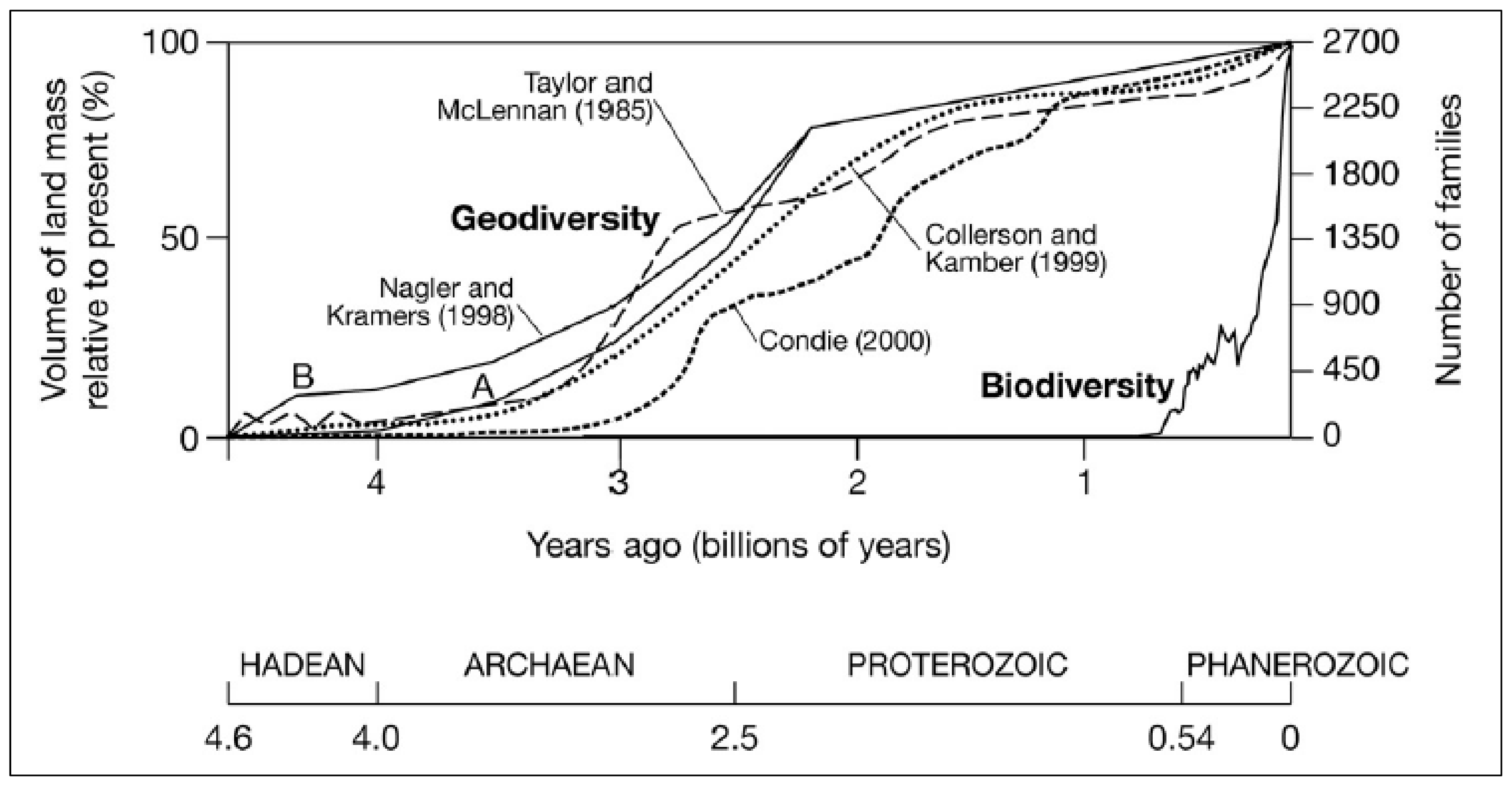


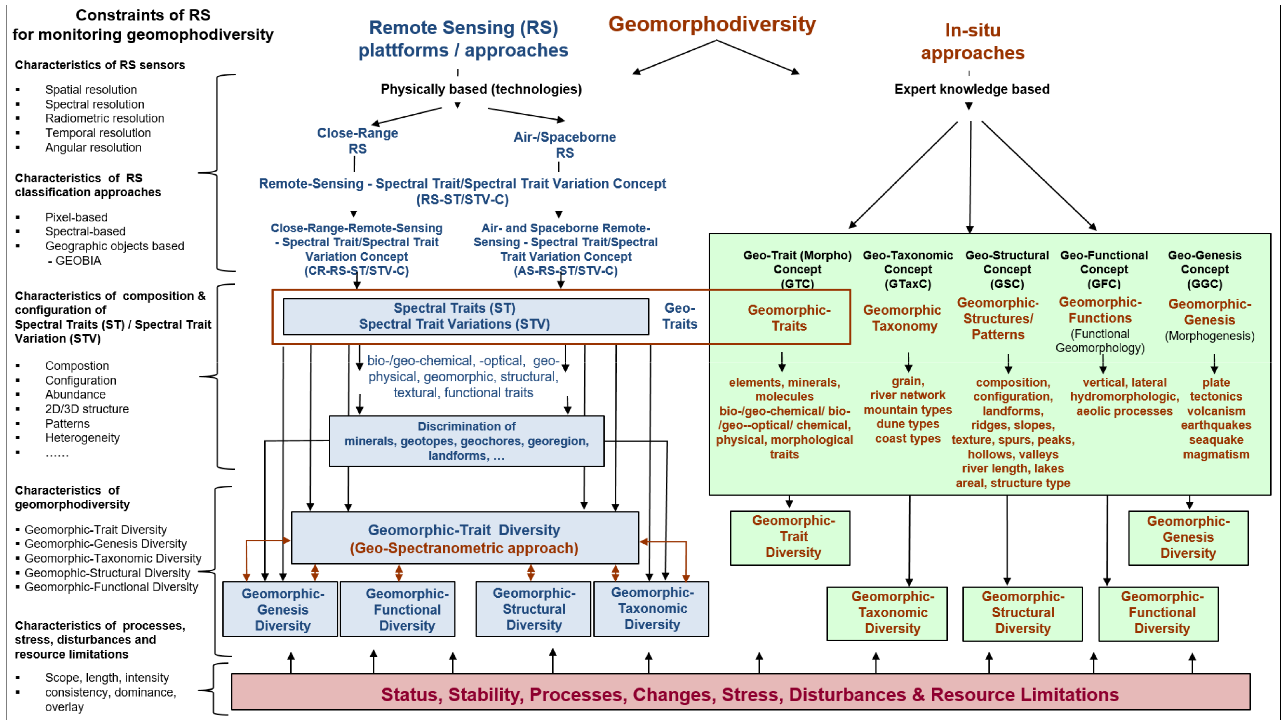
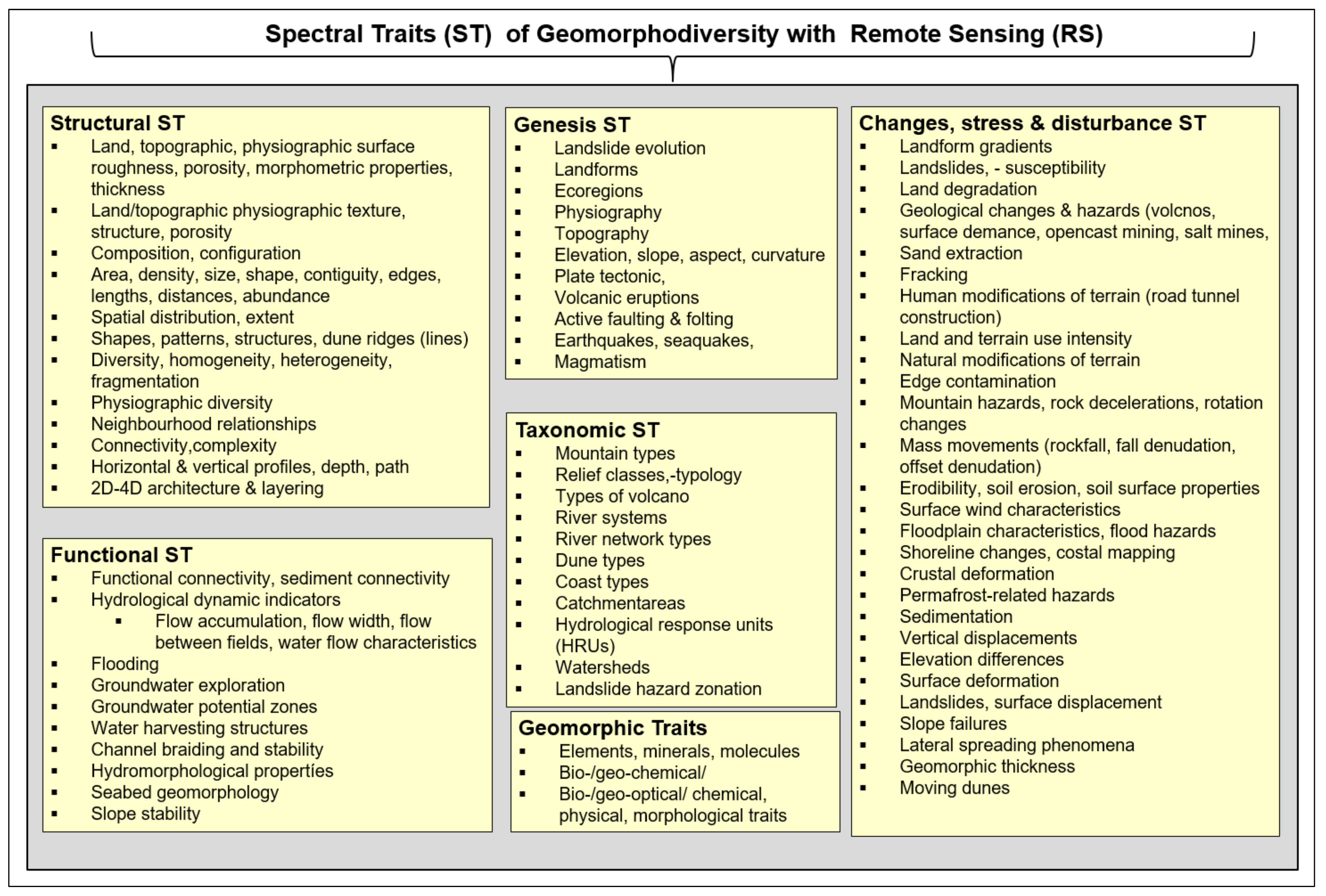


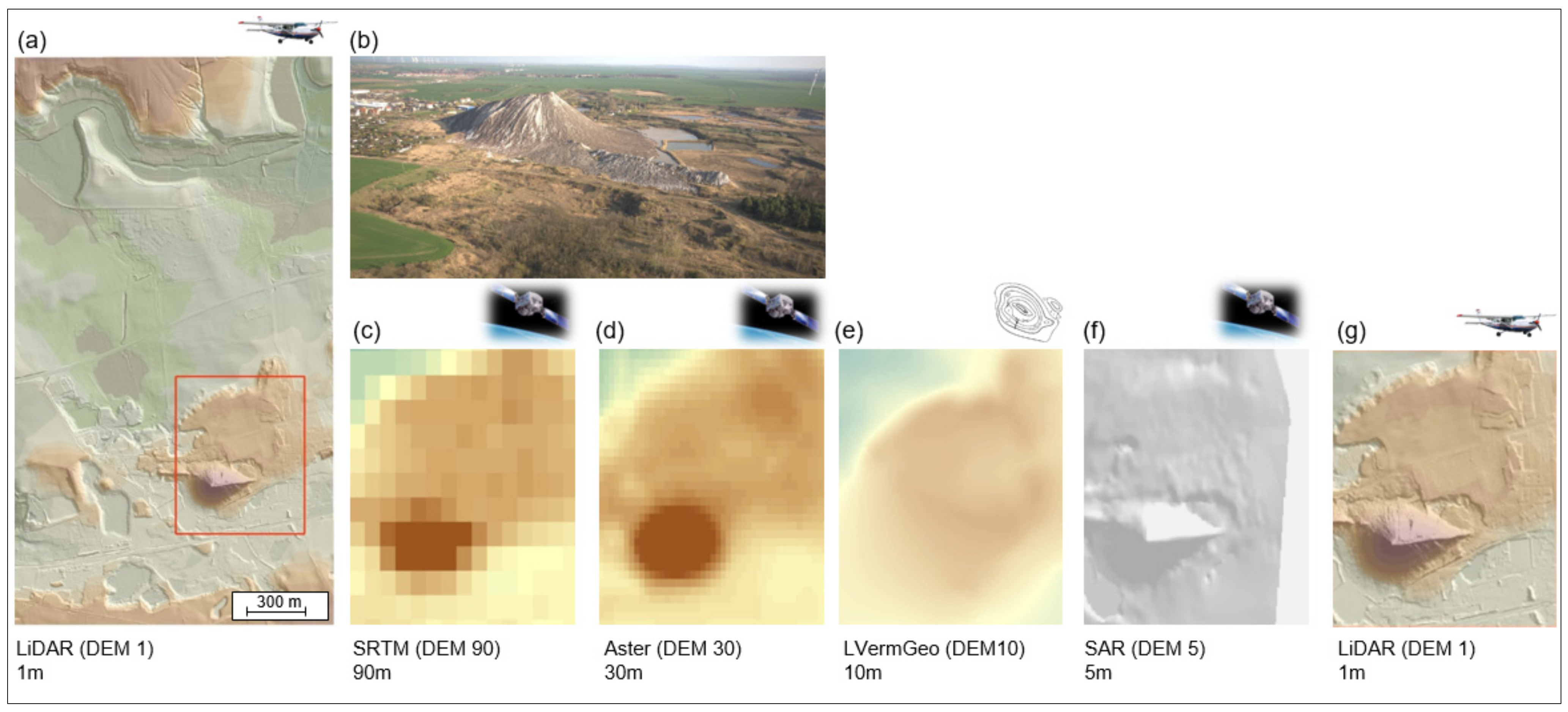

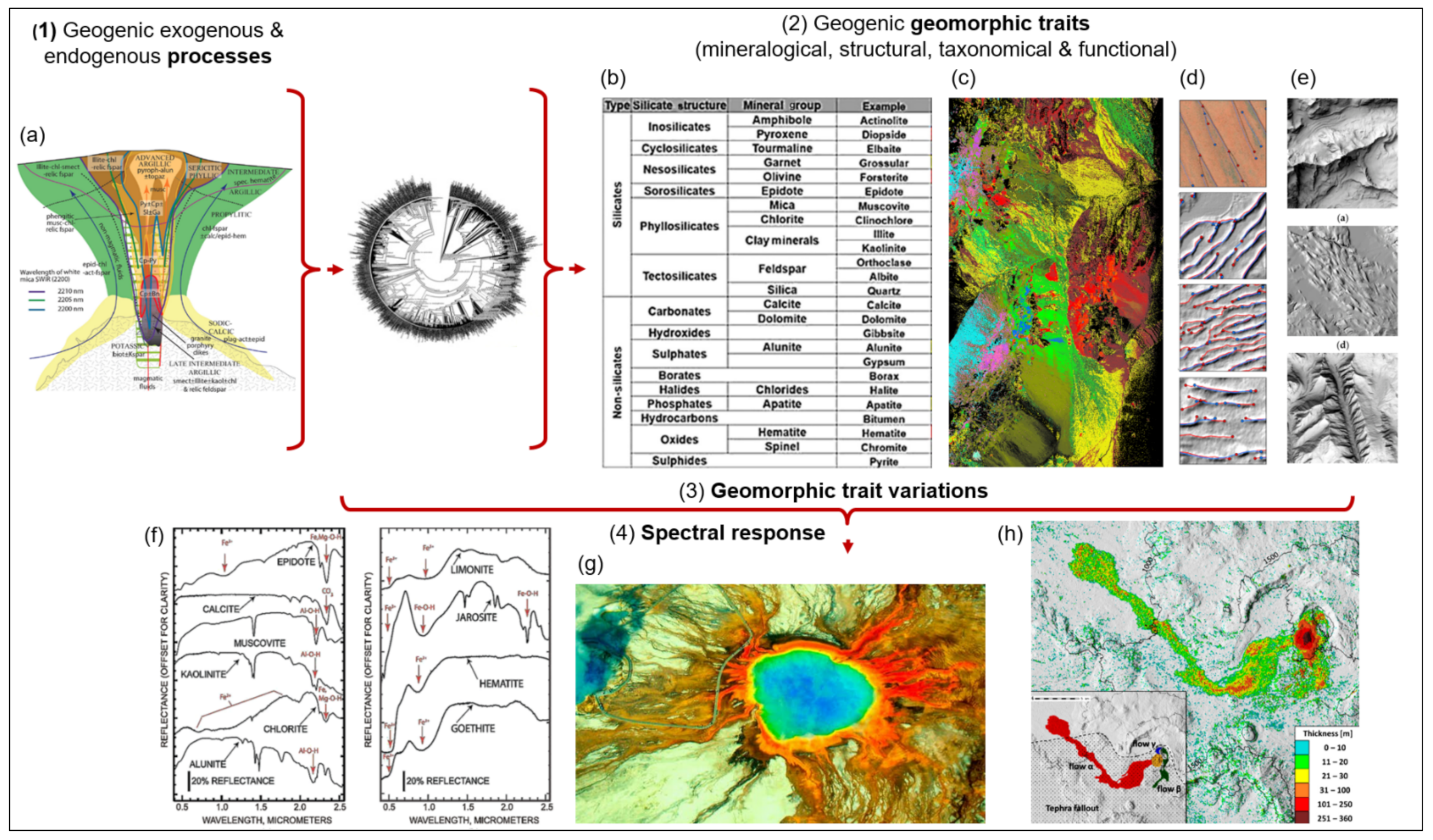


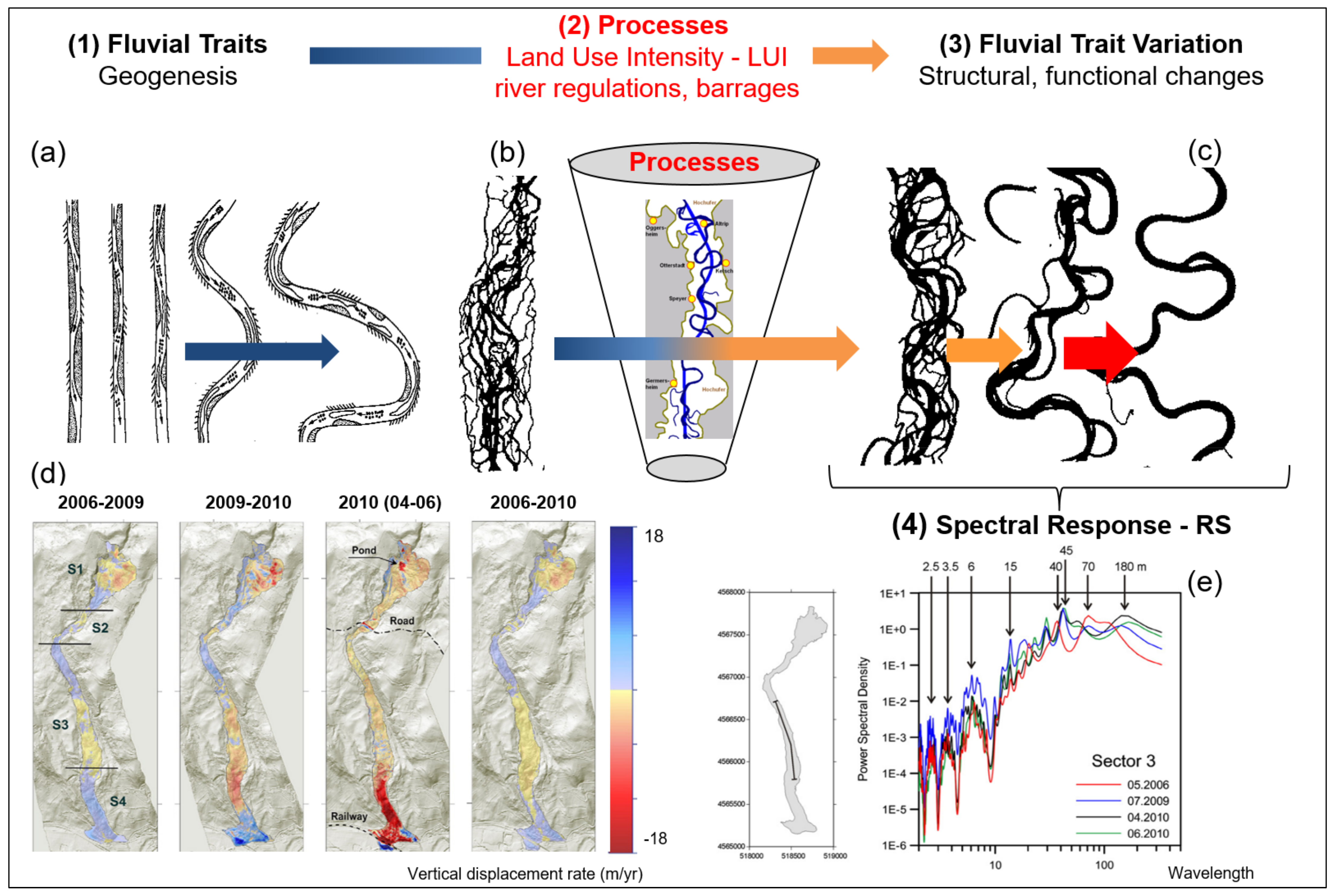

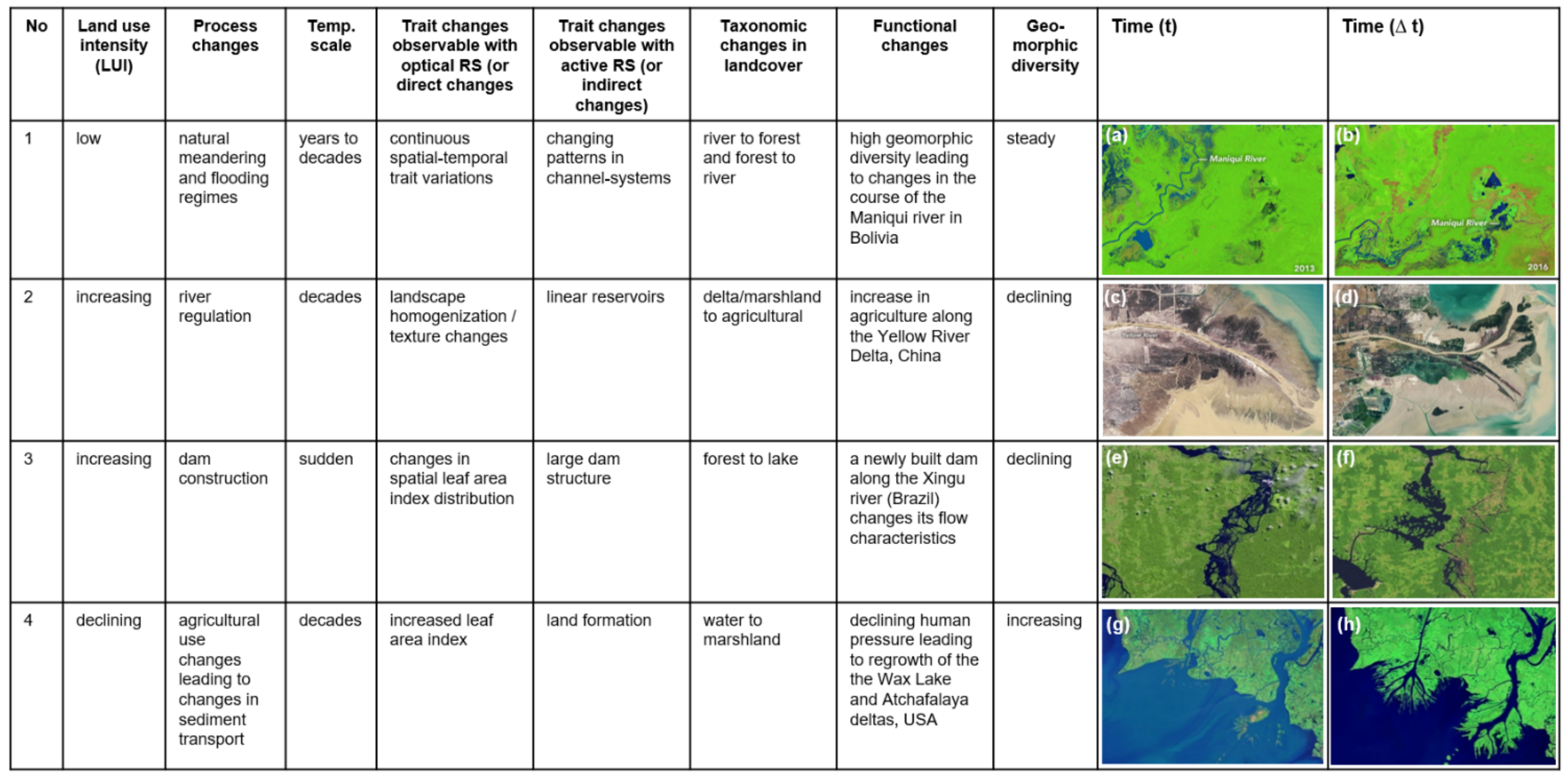

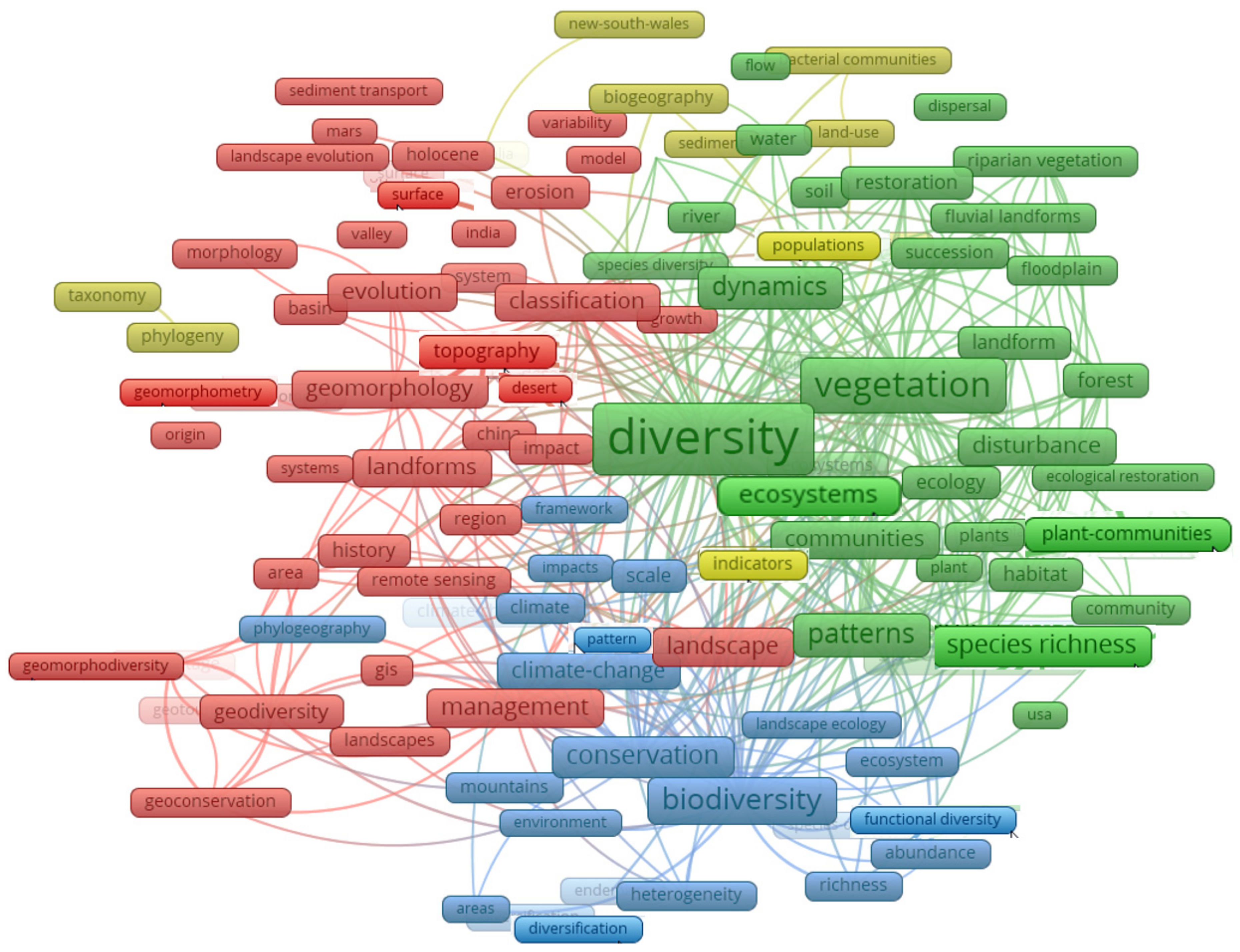
| Geomorphic—Trait Diversity | Geomorphic—Genesis Diversity | Geomorphic—Structural Diversity | Geomorphic—Taxonomic Diversity | Geomorphic—Functional Diversity | |
|---|---|---|---|---|---|
| LiDAR/GEDI | |||||
| Advantage | Sensitive to height-/topography-related traits | Direct record of top of surface changes | Simple and straightforward detection of surface structures | Depending on point density, a diversity of geomorphic components detectable | Direct surface functions assessed |
| Disadvantage | Cloud affected | Only fast genesis detectable so far | Limited spatial extent | Limited penetration capabilities to access all geomorphic components | Many geomorphic functions are not measurable with LiDAR only due to function complexity |
| RADAR | |||||
| Advantage | Special sensitvity to geometry-/structure-related traits | Sub-surface gnesis also recorded | Detection of surface and sub-surface structures possible | Assessment of sub-surface components of taxonomy | Enlarging functional diversity to sub-surface phenomena |
| Disadvantage | No exact location of scattering center due to unknown penetration into natural media | Only fast genesis detectable so far | Speckle treatment necessary | Only a few taxonomy components can be assessed | Only some geomorphic functions can be assessed |
| InSAR | |||||
| Advantage | Sensitive to height-/topography-related traits | Detection of vertical genesis processes | Vertical structures detectable | Assessment of vertical components of taxonomy | Enlarging functional diversity to vertical phenomena |
| Disadvantage | Cloud-free, For long-term studies, persistent scatters are needed, but they do not occur everywhere. | Only fast genesis detectable so far | Only line-of-sight structural changes detectable | Only a few taxonomy components can be assessed | No sensitivity to surface (lateral) geomorphic functions |
| Multispectral | |||||
| Advantage | Sensitivity to surface-related geological-related traits | Longest time series (Landsat since 1978) for genesis tracking available | Multi-spectral traits indicate structural properties and dynamics at the surface | Multi-spectral traits are sensitive to several surface taxonomy components | Diversity in function reflects in several bands of the multi-spectrum |
| Disadvantage | Only surface features, no sub-surface features | Cloud cover hampers time series density | Structural diversity better mapped in 3D than in 2D | No sensitivity to non-surface taxonomy components | Water-related functional diversity easier to assess by microwaves |
| Hyperspectral | |||||
| Advantage | High sensitivity of single spectra to single traits | Genesis tracking with single spectral bands | Asessing diversity of composition by spectral bands | Covering of diversity in taxonomic components by single spectral bands | Spectral band diversity can detect functional diversity of the surface |
| Disadvantage | Only surface features, no sub-surface features | Longer time series missing | Complicate to assess 2D to 4D geomorphic structural traits | Only diversity of surface components can be assessed | No penetration into media—only to functional diversity of surfaces |
| Thermal—TIR | |||||
| Advantage | Sensitivity to energy-/temperature-related traits | Detection of thermal genesis possible | Composition diversity can only be assessed in the TIR range (e.g., hot lava) | Temperature-related taxonomy components detectable | Functional diversity expressed in thermal variation observable |
| Disadvantage | Cloud cover hampers time series density | Longer time series missing | Only structural diversity seen at TIR is detectable | Mass/water-related geomorphic components not detected | Only temperature-related functional diversity monitored |
| MAAP | |||||
| Advantage | Ready to use multi-source data portal and algorithm developer environment | -/- | Assessing diversity of biomass structure | -/- | -/- |
| Disadvantage | Above ground biomass (AGB) as main variable | -/- | Only focused on AGB | -/- | -/- |
| Multiple in situ/RS approaches | |||||
| Advantage | Highly adaptable due to in situ knowledge | Detection of complex genesis processes enabled | Complex structural diversity detectable | Complex taxonomy components can be assessed | Geomorphic functions and their intra- and inter-specific interactions can be assessed |
| Disadvantage | Only applicable on a small spatial scale where in situ data is available | Separation of different overlapping genesis processes | Dependence on in situ site conditions and their traits | In situ data-determined assessability of taxonomy components | Applicability reduced to sites with in situ measurements |
| Dimensions | Rock | Climate | Relief | Water | Soil | Vegetation | Animals | Natural Space |
|---|---|---|---|---|---|---|---|---|
| Global | Lithosphere | Atmosphere | Geomorpho-sphere | Hydrosphere | Pedosphere | Phytosphere | Zoosphere | Geosphere |
| Zonal | - | Climatezone | - | Pedozone | Phytozone | - | Landscape zone | |
| Region | Rock region | Climate region | Geomorpho-region | Hydroregion | Pedoregion | Phytoregion | Zoo region | Landscape region |
| Megachoric | Substrate-megachore | Climate-megachore | Geomorpho-megachore | Hydro-megachore | Pedo-megachore | Phyto-megachore | Zoo-megachore | Geo-megachore |
| Macrochoric | Substrate macrochore | Climate-macrochore | Geomorpho-macrochore | Hydro-macrochore | Pedo-macrochore | Phyto-macrochore | Zoo-macrochore | Geomorpho-macrochore |
| Mesochoric | Substrate mesochore | Climate-mesochore | Geomorpho-mesochore | Hydro-mesochore | Pedo-mesochore | Phyto-mesochore | Zoo-mesochore | Geo-mesochore |
| Microchoric | Substrate-microchore | Climate microchore | Geomorpho-microchore | Hydro-microchore | Pedo-microchore | Phyto-microchore | Zoo microchore | Geo-microchore |
| Nanochoric | Substrate nanoochore | Climate nanoochore | Geomorpho-nanoochore | Hydro-nanoochore | Pedo-nanoochore | Phyto-nanoochore | Zoo-nanoochore | Geo-nanoochore |
| Topic | Substrate top | Climatetop | Geomorpho-top | Hydrotop | Pedotop | Phytotop | Zootop | Geotop |
Publisher’s Note: MDPI stays neutral with regard to jurisdictional claims in published maps and institutional affiliations. |
© 2022 by the authors. Licensee MDPI, Basel, Switzerland. This article is an open access article distributed under the terms and conditions of the Creative Commons Attribution (CC BY) license (https://creativecommons.org/licenses/by/4.0/).
Share and Cite
Lausch, A.; Schaepman, M.E.; Skidmore, A.K.; Catana, E.; Bannehr, L.; Bastian, O.; Borg, E.; Bumberger, J.; Dietrich, P.; Glässer, C.; et al. Remote Sensing of Geomorphodiversity Linked to Biodiversity—Part III: Traits, Processes and Remote Sensing Characteristics. Remote Sens. 2022, 14, 2279. https://doi.org/10.3390/rs14092279
Lausch A, Schaepman ME, Skidmore AK, Catana E, Bannehr L, Bastian O, Borg E, Bumberger J, Dietrich P, Glässer C, et al. Remote Sensing of Geomorphodiversity Linked to Biodiversity—Part III: Traits, Processes and Remote Sensing Characteristics. Remote Sensing. 2022; 14(9):2279. https://doi.org/10.3390/rs14092279
Chicago/Turabian StyleLausch, Angela, Michael E. Schaepman, Andrew K. Skidmore, Eusebiu Catana, Lutz Bannehr, Olaf Bastian, Erik Borg, Jan Bumberger, Peter Dietrich, Cornelia Glässer, and et al. 2022. "Remote Sensing of Geomorphodiversity Linked to Biodiversity—Part III: Traits, Processes and Remote Sensing Characteristics" Remote Sensing 14, no. 9: 2279. https://doi.org/10.3390/rs14092279
APA StyleLausch, A., Schaepman, M. E., Skidmore, A. K., Catana, E., Bannehr, L., Bastian, O., Borg, E., Bumberger, J., Dietrich, P., Glässer, C., Hacker, J. M., Höfer, R., Jagdhuber, T., Jany, S., Jung, A., Karnieli, A., Klenke, R., Kirsten, T., Ködel, U., ... Baatz, R. (2022). Remote Sensing of Geomorphodiversity Linked to Biodiversity—Part III: Traits, Processes and Remote Sensing Characteristics. Remote Sensing, 14(9), 2279. https://doi.org/10.3390/rs14092279