Article

Biogeochemical Model Optimization by Using Satellite-Derived Phytoplankton Functional Type Data and BGC-Argo Observations in the Northern South China Sea

1
State Key Laboratory of Tropical Oceanography, South China Sea Institute of Oceanology, Chinese Academy of Sciences, Guangzhou 510301, China
2
College of Earth and Planetary Sciences, University of Chinese Academy of Sciences, Beijing 100049, China
3
Southern Marine Science and Engineering Guangdong Laboratory (Guangzhou), Guangzhou 511458, China
4
Guangdong Key Laboratory of Ocean Remote Sensing, South China Sea Institute of Oceanology, Chinese Academy of Sciences, Guangzhou 511458, China
5
State Key Laboratory of Satellite Ocean Environment Dynamics, Second Institute of Oceanography, Ministry of Natural Resources, Hangzhou 310012, China
6
State Key Laboratory of Marine Environmental Science, Xiamen University, Xiamen 361005, China
7
Centre for Geography and Environmental Science, College of Life and Environmental Sciences, Penryn Campus, University of Exeter, Penryn TR10 9EZ, UK
8
Plymouth Marine Laboratory, Plymouth PL1 3DH, UK
9
National Centre of Earth Observation, Plymouth Marine Laboratory, Plymouth PL1 3DH, UK
*
Author to whom correspondence should be addressed.
Remote Sens. 2022, 14(5), 1297; https://doi.org/10.3390/rs14051297
Submission received: 5 January 2022 / Revised: 1 March 2022 / Accepted: 5 March 2022 / Published: 7 March 2022
(This article belongs to the Section Ocean Remote Sensing)

Abstract

:
Marine biogeochemical models have been widely used to understand ecosystem dynamics and biogeochemical cycles. To resolve more processes, models typically increase in complexity, and require optimization of more parameters. Data assimilation is an essential tool for parameter optimization, which can reduce model uncertainty and improve model predictability. At present, model parameters are often adjusted using sporadic in-situ measurements or satellite-derived total chlorophyll-a concentration at sea surface. However, new ocean datasets and satellite products have become available, providing a unique opportunity to further constrain ecosystem models. Biogeochemical-Argo (BGC-Argo) floats are able to observe the ocean interior continuously and satellite phytoplankton functional type (PFT) data has the potential to optimize biogeochemical models with multiple phytoplankton species. In this study, we assess the value of assimilating BGC-Argo measurements and satellite-derived PFT data in a biogeochemical model in the northern South China Sea (SCS) by using a genetic algorithm. The assimilation of the satellite-derived PFT data was found to improve not only the modeled total chlorophyll-a concentration, but also the individual phytoplankton groups at surface. The improvement of simulated surface diatom provided a better representation of subsurface particulate organic carbon (POC). However, using satellite data alone did not improve vertical distributions of chlorophyll-a and POC. Instead, these distributions were improved by combining the satellite data with BGC-Argo data. As the dominant variability of phytoplankton in the northern SCS is at the seasonal timescale, we find that utilizing monthly-averaged BGC-Argo profiles provides an optimal fit between model outputs and measurements in the region, better than using high-frequency measurements.

1. Introduction

Numerical models play a vital role in investigating complex marine ecosystem dynamics. Numerical models require multiple parameters to formulize the ecological processes, but it is often difficult to constrain model parameters. As the complexity of a marine model increases, thus does the number of model parameters. Constraining model parameter values and their uncertainties have a great influence on model performance [1,2], and one way of doing that is through data assimilation. Assimilating ocean remote sensing observations into the model to adjust model parameters and reduce their uncertainties can help towards a better representation of marine ecosystem dynamics [3,4,5,6,7,8,9].
Processes of growth, decay, and interaction by plankton are important in understanding marine ecosystem models and dynamics. Model parameters related to these processes are usually tuned empirically and arbitrarily. In order to reproduce observed data such as the distribution of phytoplankton and analyze underlying dynamics, it is required to reasonably estimate model parameters. Here, we developed and optimized a physical-biogeochemical model in the South China Sea (SCS) to study phytoplankton distributions and dynamics. The SCS is a large semi-enclosed marginal sea in the western Pacific. In winter, the SCS is dominated by the strong northeasterly monsoon, whereas in summer the winds reverse direction to southwesterly. The seasonal change of monsoon winds leads to variability in the upper ocean circulation [10,11]. The dominant temporal variability of biogeochemical processes in the upper ocean occurs on the seasonal time-scale [12]. Ning et al. [13] reported low surface production in summer and high in winter. In the northern SCS, previous studies showed a negative correlation between satellite-derived chlorophyll-a concentration (Chla) and sea surface temperature [14,15]. Recently, Geng et al. [16] demonstrated that the buoyancy flux induced mixing controls the seasonal variability of vertical nutrient transport and phytoplankton production in the northern SCS.
The winter mixing also has the potential to shoal the subsurface chlorophyll-a maximum (SCM) and change the vertical distribution of chlorophyll-a [16,17]. The SCM is a common feature in the northern SCS, contributing significantly to the depth-integrated primary production [18]. The formation and maintenance of SCM in the SCS have been investigated with idealized models [16,17,19], which identified key factors such as detritus remineralization, zooplankton grazing, phytoplankton sinking, and phytoplankton photoacclimation in modulating the SCM. However, the relative importance of these processes is largely determined by their parameterizations in the model. Rigorously quantifying processes that influence vertical distributions of chlorophyll-a thus requires a prior optimization of the model parameters.
Satellite-derived chlorophyll-a concentration has been widely used to constrain or evaluate biogeochemical models. However, ocean color satellites only detect the near-surface. The SCM is generally located at ~75 m in the northern SCS [16], which is far beyond the detection depth of satellites. In addition, satellite-derived chlorophyll-a is the bulk value of the near-surface water. It can be used to constrain the biogeochemical model that only simulates one phytoplankton group. For biogeochemical models with multiple phytoplankton groups or sizes, large uncertainties exist when using the satellite-derived bulk chlorophyll-a concentration to constrain the model, as additional assumptions are required on the relative contributions of phytoplankton groups [20,21,22,23].
Recent advances in estimating phytoplankton functional type (PFT) from satellite provides an opportunity to constrain models with multiple phytoplankton groups [24,25]. The PFT models are mostly derived from in situ High Performance Liquid Chromatography (HPLC) pigment data. Pigments determined by HPLC can be found in a variety of phytoplankton taxa and size classes, which may introduce uncertainties in the PFT model. For satellite PFT data, per-pixel uncertainties are generally difficult to quantify, especially in regions that are not covered by satellite and in situ match-up datasets [25]. Additional uncertainties can also occur because of differences in the temporal and spatial scales between satellite and in-situ data. Nevertheless, assimilation of PFT in the model has been shown to improve the simulation of phytoplankton community structure and produce a better total chlorophyll-a forecast in the North Atlantic [26,27]. Studies provide a PFT-based eco-regionalization of the Mediterranean Sea [28] and improve the simulation of PFT in the global ocean [29]. Biogeochemical-Argo (BGC-Argo) floats are able to sample the ocean vertically and continuously. Wang et al. [9] reported that assimilating profiles sampled by a BGC-Argo float yielded significant improvements for both surface and subsurface chlorophyll-a simulation. Utilizing both satellite PFT and BGC-Argo data in multi-phytoplankton biogeochemical models may thus have great potential in adjusting model parameters.
In this study, a one-dimensional (1D) physical-biogeochemical model has been developed in the northern SCS. By using a genetic algorithm, we investigate the value of using satellite PFT and BGC-Argo data to optimize model parameters. The aim of this study is to improve the simulation of vertical distributions of phytoplankton chlorophyll-a and particulate organic carbon (POC) concentrations in the northern SCS. Due to the computational cost, parameter optimization in a three-dimensional (3D) model is challenging. However, parameters optimized by using the 1D model can provide a useful baseline for 3D modeling [9,30,31].

2. Methods

2.1. Model Description

A coupled physical–biogeochemical model was developed in the northern SCS. The physical model is based on the Regional Ocean Modeling System (ROMS), which represents an evolution in the family of terrain-following vertical-coordinate models [32]. The model was set up with 100 layers in the vertical direction. The Mellor–Yamada Level 2.5 turbulence closure scheme was used in the model. The 1D model only considers vertical mixing processes without advection. Although it is simplified, previous studies have shown that the 1D coupled model can simulate vertical structures of biogeochemical variables reasonably well in the SCS basin [16,17]. The biogeochemical model is based on the Carbon, Silicate, and Nitrogen Ecosystem (CoSiNE) model, which has been calibrated and configured in the SCS [33,34]. The model has 2 phytoplankton groups (pico-phytoplankton (S1, Chl1) and diatoms (S2, Chl2)), 2 zooplankton groups (micro-zooplankton (Z1), mesozooplankton (Z2)), 2 size classes of particulate organic nitrogen (small (SPON), large (LPON)), biogenic silica (bSi), 4 inorganic nutrients (nitrate (NO3), ammonium (NH4), phosphate (PO4), silicate (Si(OH)4)), dissolved oxygen (DO), and carbonate variables (dissolved inorganic carbon (DIC), total alkalinity (TALK)). In addition to the nitrogen-based biomass of phytoplankton, phytoplankton chlorophyll concentration for each group (pico-phytoplankton and diatom) was modeled following Geider et al. [35] by considering phytoplankton photo-acclimation with variable chlorophyll to biomass ratio. Nutrients such as nitrate, ammonium, and phosphate determine the growth of phytoplankton. Silicate is the additional nutrient that controls the growth of diatoms. Microzooplankton grazes on pico-phytoplankton, while mesozooplankton grazes on diatoms, microzooplankton, and detritus. The mortality and aggregation of phytoplankton and zooplankton form detritus, which are remineralized into inorganic matters during sinking. The 2 sizes of detritus were parameterized with different sinking speeds and remineralization rates. Model equations are as follows:
C t = P H Y ( C ) + B I O ( C ) ,
where C represents the concentration of a biological variable. PHY(C) represents the contribution to the concentration change due to physical processes. BIO(C) represents biogeochemical source-minus-sink terms. The detailed equations are presented in Appendix A and the original model parameters are listed in Ma et al. [34].
The CoSiNE model has the capability of simulating 2 phytoplankton functional groups, pico-phytoplankton and diatom, which are 2 dominant phytoplankton groups in the northern SCS. Resolving phytoplankton functional groups in the model is important for realistic simulations of nutrient and carbon dynamics, because diatom-related aggregation and grazing processes tend to generate large particles that sink faster and remineralize deeper than the pico-phytoplankton related processes. As a consequence, biogeochemical models with 1 phytoplankton group may have difficulties in reasonably simulating the vertical distribution of the remineralization process of particulate organic matter, which can further lead to model bias in nutrient and carbon distributions. Furthermore, the CoSiNE model has been applied and validated in the SCS in many different studies. It has been used to study mesoscale eddies [36], Kuroshio intrusion fronts [37], carbon export [34], and cross-shelf exchange [38], etc., which shows its applicability in the SCS. Because of the model’s ability in simulating two phytoplankton groups, we were able to utilize both satellite-derived PFT data and total chlorophyll-a concentration to constrain the model.
The coupled model was initialized with the climatological data from the World Ocean Atlas 2009 (WOA09) and was forced by the 6-hourly surface forcing fields from NCEP/NCAR reanalysis data, including air temperature at 2 m, surface wind components at 10 m, relative humidity at 2 m, sea level pressure, total cloud coverage, and net short- and long-wave radiations. The model was run for 4 years from January 2013 to December 2016.
The model was set up at the South East Asian Time series Study (SEATS; 18° N, 116° E) station in the northern SCS (Figure 1). The SEATS is a station that is representative of typical physical and biogeochemical conditions in the northern SCS. The SEATS station is located away from coastal upwelling regions in the SCS [39,40,41]. The major nutrient supply to the upper layers is via vertical mixing [42]. The seasonal change of monsoon winds leads to variability in the upper ocean circulation. The dominant temporal variability of biogeochemical processes in the upper ocean occurs at the seasonal timescale, and surface production stays low in summer and high in winter. In the SCS, mesoscale eddies are ubiquitous, which have an important influence on the biological process, but eddies are often sporadic and do not show a clear seasonal pattern in the northern SCS [43]. Therefore, the influence of eddies is not discussed in the parameter optimization process in this study.

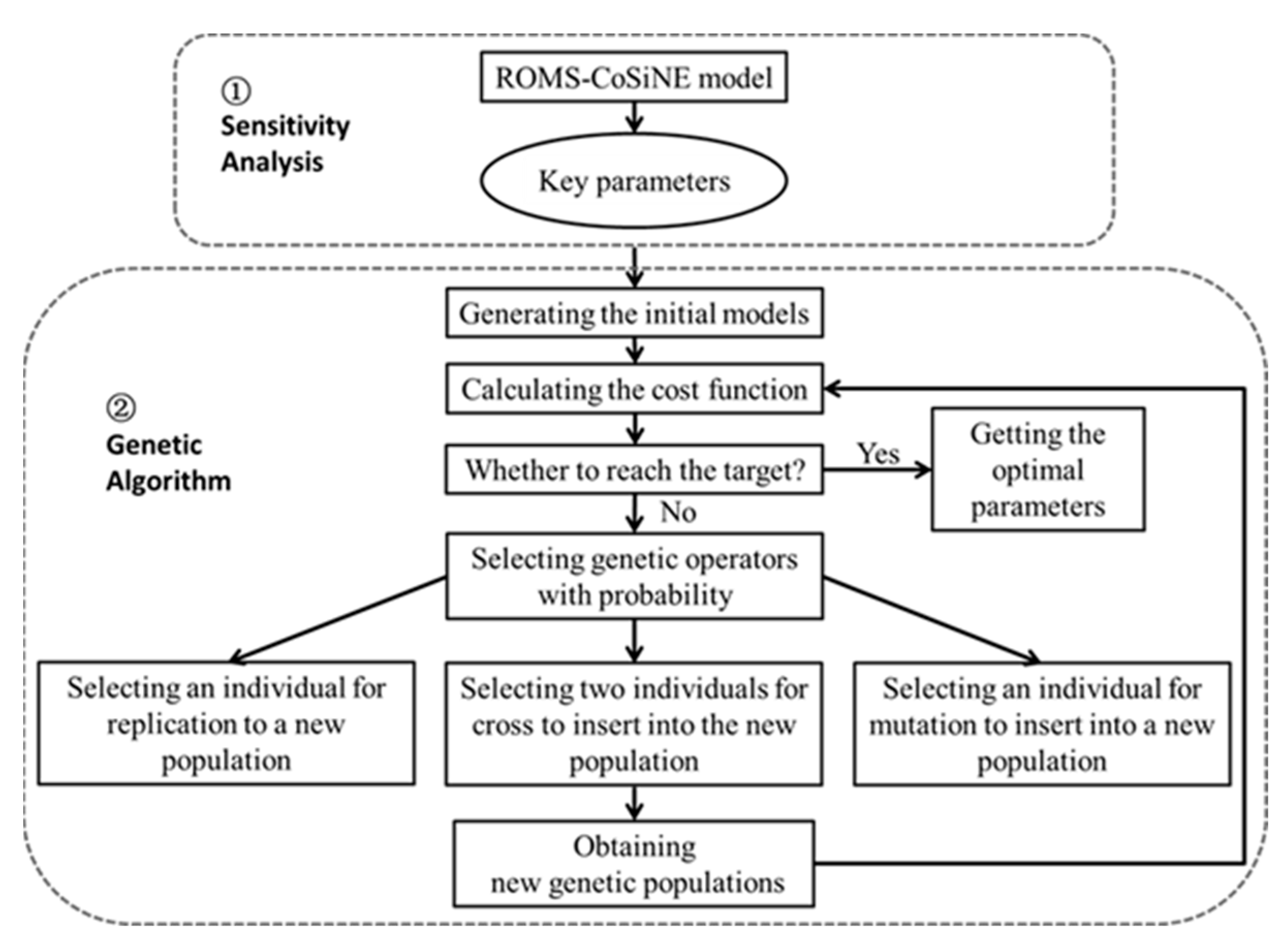
2.2. Sensitivity Analysis

There are more than 40 parameters related to biochemical processes in the CoSiNE model. Parameters with high sensitivity should have priority for optimization. Therefore, a sensitivity analysis was carried out first to identify the parameters that have an important influence on modeled chlorophyll-a concentration. The initial parameter values refer to previous studies [34,44,45,46], and possible ranges for each parameter, before the optimization, were defined following the method of Hemmings et al. [47] and Kaufman et al. [31]. The upper and lower bounds for biological parameters, such as parameters related to phytoplankton growth and zooplankton grazing, were selected from the rules of previous studies [31,47]. For the parameters that were unique in the CoSiNE model, bounds were set to be half and double the initial values. For fractional parameters, values were set to vary from 0.05 to 0.95. The sensitivity analysis experiment was conducted in 2 steps.
Firstly, we used a sensitivity formulation to perform a screening sensitivity analysis. The following sensitivity function is employed to measure the local sensitivity of the biological parameters to model outputs [45,48]:
S C , x = C x C x % C x / X X x % X ,
where Xx−% is the value of biological parameter subtracted by a fixed ratio (50%), Cx−% is the corresponding annual mean chlorophyll-a concentration at the sea surface. Parameters with larger Sc,x values are thought to be more sensitive to the model. With this approach, we identified 20 sensitive parameters by using a threshold of Sc,x > 20%. These parameters have large impacts on phytoplankton dynamics at the SEATS station. The sensitivity of the remaining parameters was less than 20%, and the variations in phytoplankton chlorophyll-a due to these insensitive parameters were small, thus these parameters were ignored in the following analysis.
Secondly, we performed the next step of the global sensitivity analysis experiment on the sensitive parameters identified in the first step to further pick out the key parameters. We conducted an analysis following the approach of Hemmings et al. [47] for all 20 sensitive parameters using the Monte Carlo sampling methods to obtain 500 different combinations of these parameters [49,50]. The sampling ranges were the same as the parameter optimization range. Then, we conducted these 500 groups of model runs, each of which has a unique combination of parameter values. We computed the coefficient of determination (r2) between the parameter and the output of chlorophyll-a concentration at the sea surface to quantify the amount of variance in the outputs explained by each parameter. After that, we ranked the r2 of each parameter and selected the key parameters for the subsequent optimization process.

2.3. Genetic Algorithm

Genetic algorithm (GA) is a powerful tool to solve various optimization problems. It is a random search algorithm, including a process of evolving a population of individuals generated randomly towards better solutions. It is an iterative process. Each individual represents a solution to the problem and is characterized by its fitness, which shows its chance of survival. The fitness is usually the value of the objective function in the optimization problem being solved. New individuals are built by means of crossover and mutation operators. A crossover operator produces 2 offspring by combining and exchanging the elements of 2 parent individuals randomly. Mutation adds small random changes to an individual. A genetic algorithm can reduce the risk of premature convergence by re-initializing after each convergence and creating new random individuals while maintaining the best fit individual from the iterative process [51].
The input parameters of the GA contain population size, probabilistic crossover rate, probabilistic mutation rate, and the maximum number of the generation. In this study, those 4 parameters were set to be 20, 0.6, 0.1, and 1000, respectively. In this optimization algorithm, the individuals of the GA represent the CoSiNE models with different parameter sets. The fitness is denoted by the cost function, which shows the difference between the model result and observations. Genetic individuals of each generation were selected using a roulette model to generate a combination of parameters with better performance according to the pre-set crossover and mutation probability. The process of “survival of the fittest” implies a maximization procedure. The entire process is conducted to further improve the cost function until a stopping criterion is met. Possible stopping criteria are related to optimal fitness value or the maximum number of the generation. The cost function, F, is defined as:
F = 1 N i N ( x _ s i m u l a t e d x _ o b s e r v e d   ) σ 2 2 ,
where x_simulated is the simulated value, x_observed is the observations, σ is the standard deviation of the observations and N is the number of observations. The aim of GA process is to search for the best parameter combination to minimize the misfit between the observations and simulations. The flow chart of the entire model parameter optimization process is shown in Figure 2.

2.4. Data and Optimization Experiments

The observations used during the optimization process include ocean color data and BGC-Argo profiles. Ocean color-derived chlorophyll-a concentration with a horizontal resolution of 4 km was obtained from Ocean Color Climate Change Initiative (OC-CCI) dataset provided by the European Space Agency [52]. The data combines measurements from 4 sensors, including the Sea-viewing Wide Field of View Sensor (SeaWiFS), the Moderate-Resolution Imaging Spectroradiometer (MODIS), the Medium Resolution Imaging Spectroradiometer (MERIS), and the Visible Infrared Imaging Radiometer (VIIRS). Remote-sensing reflectance data from MODIS-Aqua, MERIS, and VIIRS were band-shifted to match the wavebands of SeaWiFS. The merged products were validated against in-situ observations. The uncertainties (bias and RMSD) are assigned to every pixel in the products [21]. Daily OC-CCI chlorophyll-a concentration data within a 3 × 3 pixel around the SEATS station were used. We analyzed the satellite data with in-situ measurements, and the correlation was up to 0.93 at the SEATS station. These OC-CCI chlorophyll-a data were further processed into a daily PFT dataset following previous studies of Lin et al. [24] and Brewin et al. [25], which have 3 phytoplankton groups: pico-, nano-, and micro-phytoplankton. The details of 3-component PFT model of phytoplankton size classes are shown in Appendix B. As our model only includes pico-phytoplankton and diatom, the PFT-derived nano- and micro-phytoplankton were combined to constrain the modeled diatom for the data assimilation. From these data, the ratios of pico-phytoplankton and diatom (nano- and micro-phytoplankton) chlorophyll-a concentrations to total chlorophyll-a were about 76% and 24% for the whole year, respectively. Lin et al. [24] collected remote sensing and in situ pigment data during SCS cruises from 2006 to 2012. From their measurements, the ratio of pico-phytoplankton chlorophyll-a to total chlorophyll-a concentration was between ~60% and ~80%, with slightly higher value in winter and lower in summer, which was consistent with the data used in this study. With the PFT data, the GA optimization calculated the cost function for each phytoplankton group separately thus as to achieve the goal from the total weighted F value at each generation.
A BGC-Argo float was deployed in the northern SCS on 27 June 2014 (Figure 1), profiling every 1 to 5 days with a vertical resolution of ~2 m above 1000 m and of ~50 m from 1000 to 2000 m depth. The float always surfaced near local midnight to avoid the in vivo fluorescence non-photochemical quenching [53,54]. The float was equipped with a SBE 41CP CTD and a WETLabs MCOMS 3-in-1 optical sensor that included sensors for chlorophyll-a fluorescence and the particulate backscattering coefficient at 700 nm (bbp(700)). The float data were processed following Xing et al. [55]. Near the float deployment time and location, water was collected for in situ calibration of the float’s chlorophyll-a fluorometer [55]. Before parameter optimization, we have removed abnormal outliers. The bbp(700) profiles were smoothed by a 5-point running median filter to remove unexpected spikes [56,57]. The particulate organic carbon (POC) was calculated from measured bbp(700) based on the empirical relationship [58], which was also validated in the SCS [59]:
P O C = 53,607 × b b p ( 700 ) × ( 555 / 700 ) 1 + 2.5 ,
We conducted a series of optimization experiments to assimilate the ocean color data and float observations of chlorophyll-a. In these experiments, we applied different observation data for F calculation (Table 1) and each experiment was initialized from the same individuals of the GA. In the control (CTRL) run, the model used default model parameters without data assimilation. In experiment 1 (EXP1), only satellite data were used to optimize the model. EXP1a used satellite ocean color data to compare the total sea surface chlorophyll-a from the model. EXP1b adopted ocean color PFT data to calculate the cost function for each phytoplankton group separately. In experiment 2 (EXP2), BGC-Argo profiles of chlorophyll-a from 5 m to 150 m were used. Besides, the depth-integrated chlorophyll-a between 65 m and 85 m were added into the cost function to better capture the SCM feature. In experiment 3 (EXP3), both ocean color PFT and float profiles of chlorophyll-a were used for optimization. In addition, we set up two more experiments based on EXP3. We calculated the seasonal average and monthly average of BGC-Argo profiles data for assimilation to eliminate the high-frequency effect of the floats data, and the other settings were kept consistent.

3. Results

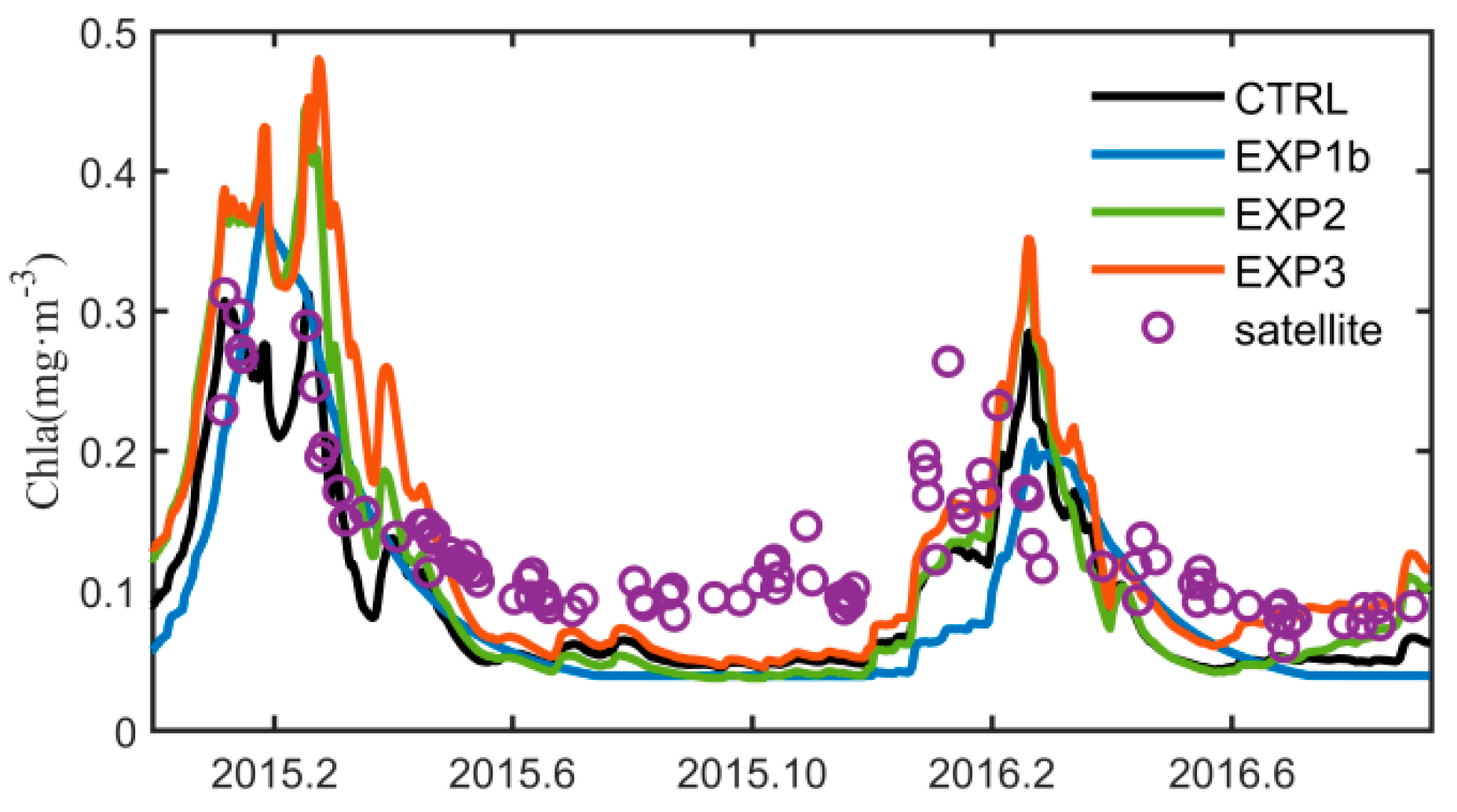
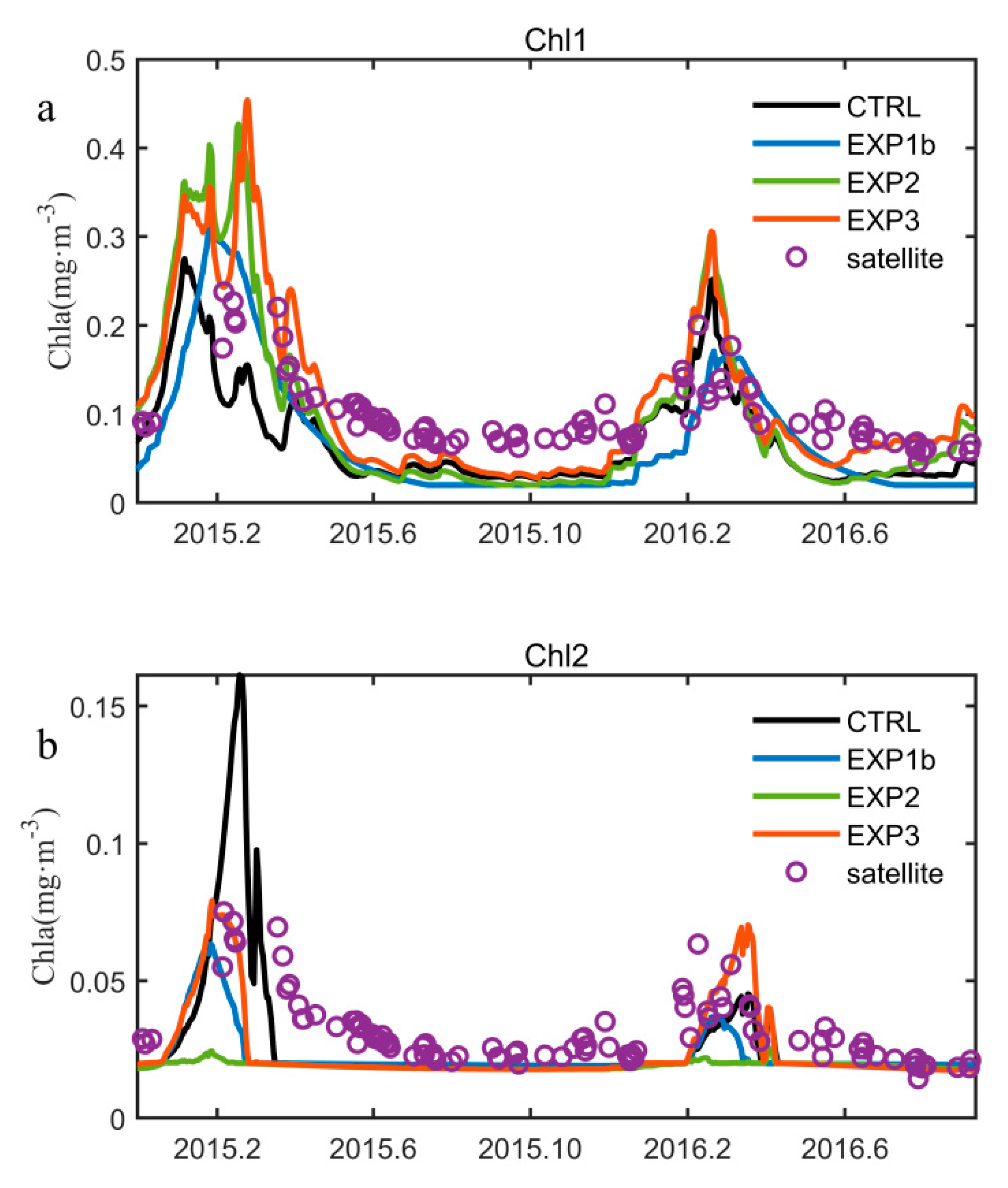
3.1. Seasonal Variation of Chlorophyll-a

Temporal variations of satellite-derived chlorophyll-a and BGC-Argo profiles are shown in Figure 3. In the surface layer, satellite-derived chlorophyll-a concentration demonstrates obvious seasonal characteristics (Figure 3a). In winter, surface chlorophyll-a concentration reaches the highest value of about 0.3 mg m−3, due to the winter cooling and strong mixing that brings subsurface nutrients into the upper layer [60]. In spring, surface chlorophyll-a decreases gradually. Surface chlorophyll-a shows a very low concentration of about 0.1 mg m−3 in summer, resulting from nutrient depletion at the surface and enhanced vertical stratification [14]. Chlorophyll-a concentration stays low during the monsoon transition period.
From BGC-Argo float profile data, sea surface chlorophyll-a shows the same feature. Sea surface chlorophyll-a is highest in winter and relatively low in other seasons (Figure 3b). The winter peak of chlorophyll-a from the float is a little higher than that from the satellite data. Zhang et al. [61] found this same phenomenon by comparing BGC-Argo chlorophyll-a at 5 m depth with remote sensing derived data obtained by MODIS/Aqua instruments. It might be because that the float covered a relatively wide spatial range with high phytoplankton biomass area in the northern SCS (Figure 1). There is also uncertainty in remote sensing reflectances (Rrs). Products derived from Rrs are affected by the bias to varying degrees, with chlorophyll varying up to 25% over a year [62,63]. On the other hand, satellite observations may miss high chlorophyll-a peaks due to cloud influence in winter. Other than this small difference, the BGC-Argo chlorophyll-a data are in agreement with remote sensing data.
In the northern SCS, SCM exists but is less significant in winter, demonstrating a seasonal variation. A distinct SCM appears in spring, gradually deepens in summer and autumn with a value of more than 0.6 mg m−3 and a depth of 65–85 m, consistent with the model result and observations of Gong et al. [17]. The SCM quickly shoals or even disappears in winter and surface phytoplankton reaches high concentrations. The SCM in the northern SCS is affected by multiple biological processes, such as phytoplankton growth, zooplankton grazing, phytoplankton sinking, phytoplankton photo-acclimation and detritus remineralization [17,61,64]. Parameter optimization could facilitate the ecosystem model to reproduce the SCM and better elucidate dominant dynamics of phytoplankton chlorophyll-a distribution.

3.2. Optimizable Parameter Selection

We first identified 20 sensitive model parameters based on the sensitivity analysis. Considering the sensitivity of modeled surface chlorophyll-a concentration, parameters related to zooplankton grazing, phytoplankton growth, and detritus remineralization are particularly sensitive. Then we conducted 500 groups of model runs with a unique combination of parameter values using the Monte Carlo sampling as described in Section 2.2.
According to the analysis above, 9 key parameters (Table 2) were selected for the model set up in the northern SCS, which mainly fell into 3 categories: predator-related parameters for zooplankton, growth-related parameters for phytoplankton and the initial slope of the P-I curve associated with phytoplankton photosynthesis. The GA optimization aims at these 9 optimizable parameters and searches for the best parameter combination to minimize the misfit between the observations and simulations.

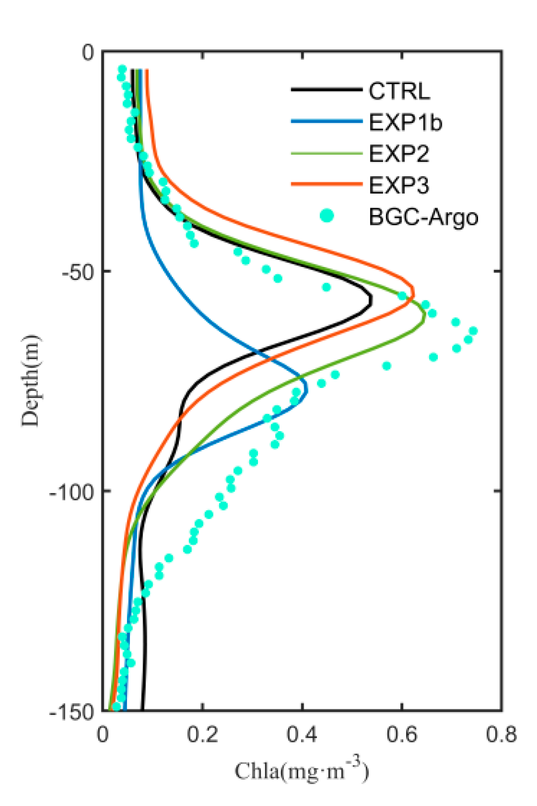
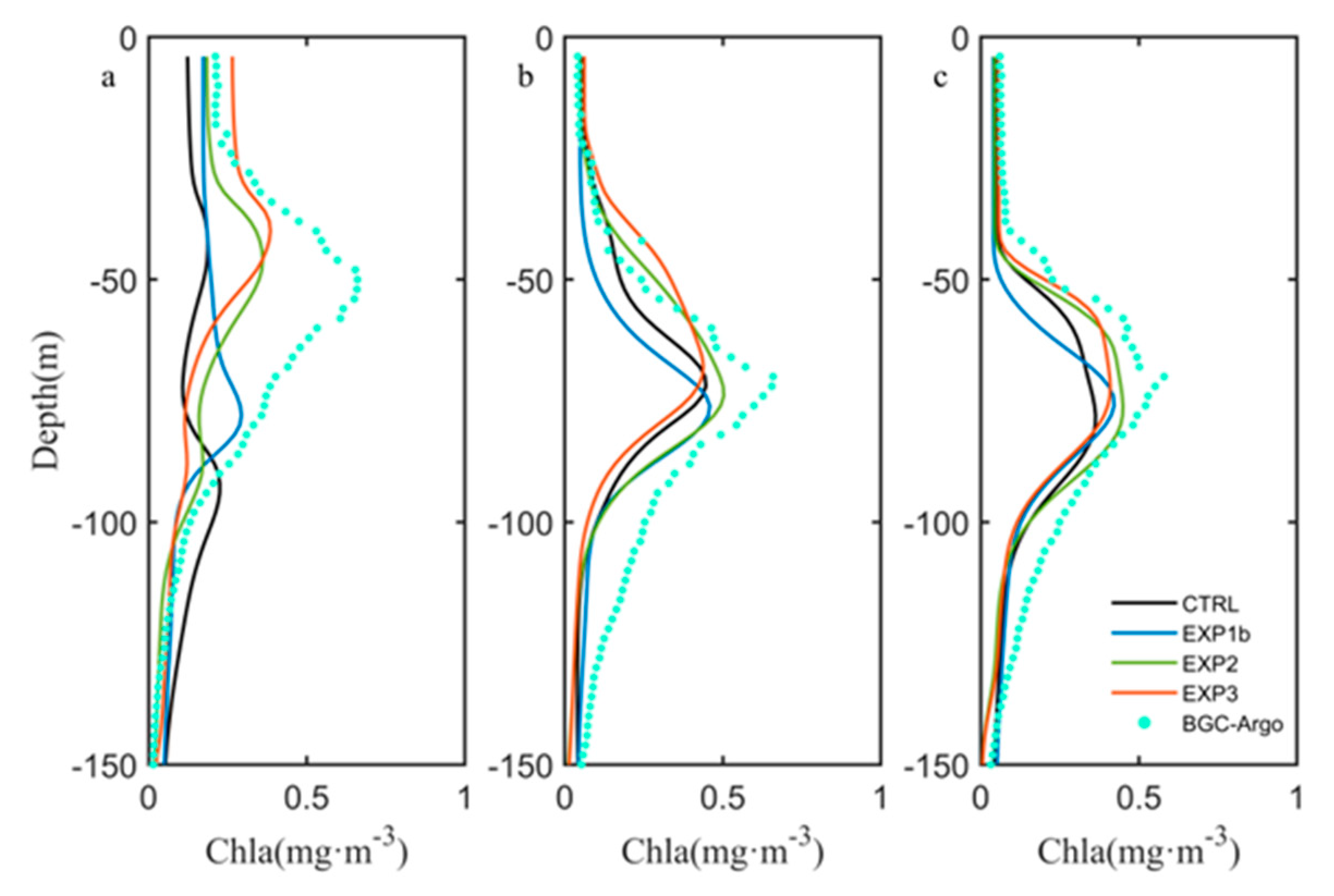
3.3. Optimization Results

The default parameters in the CoSiNE model have been empirically tuned against different observations in the SCS [34]. Nevertheless, compared with the CTRL run, assimilating data into the model using the GA showed improvements in the cost function for all runs (Table 3). The cost function of each experiment varied with the data assimilation settings.
In EXP1, assimilation of satellite data improves the model result of sea surface chlorophyll-a and phytoplankton groups. The EXP1a, directly incorporating the satellite chlorophyll-a in the optimization, decreases the cost function by 5.3%. From Table 3, both Fs1 and Fs2 in EXP1a display reductions, suggesting that adjustment of total chlorophyll-a improves the chlorophyll-a simulation contributed by different phytoplankton functional types. However, the vertical simulation of chlorophyll-a is not improved in EXP1a. Compared with EXP1a, EXP1b shows a better performance in reproducing two phytoplankton functional types, indicating ocean color PFT data assimilation has the potential to improve estimation of phytoplankton groups. The cost function values of the two phytoplankton functional types in EXP1b decrease by 26.8% and 49.2%, respectively. In the northern SCS, chlorophyll-a concentration of pico-phytoplankton is typically higher than diatoms [65]. Although modeled total chlorophyll-a concentration fits well with ocean color data (Figure 4), the CTRL model predicts a larger concentration of diatom group, resulting in the diatom ratio being significantly higher in winter, even up to 50% (Figure 5). After the assimilation of PFT, the relative ratio of diatom in EXP1b is more consistent with observations. However, the model misses the vertical distribution pattern of chlorophyll-a, with a deeper but smaller SCM (Figure 6). It indicates that while the assimilation of satellite data improves the model predictions of phytoplankton groups at the surface, the model predictions of vertical chlorophyll-a structure may still not be optimal compared with the CTRL run (Table 3), likely due to the lack of vertical information.
In EXP2, the modeled vertical chlorophyll-a profile matches the observations quite well (Figure 6). The cost function value of chlorophyll-a averaged over the water column between model and observations declined by 20.4% (Table 3). Compared to the CTRL and EXP1, the assimilation of vertical float observations largely improves subsurface predictions of chlorophyll-a. The magnitude and the vertical location of SCM are more consistent with the float data. The model reproduces the seasonal variation of surface total chlorophyll-a concentration (Figure 4). However, it fails to simulate surface phytoplankton groups, especially for diatom, with its concentration considerably low in the whole modeling period (Figure 5). Since the chlorophyll-a of pico-phytoplankton dominates the total chlorophyll-a, underestimation of diatom might be neglected if only considering total surface chlorophyll-a. In Figure 4, each model exhibits reasonable prediction of the surface chlorophyll-a. However, the phytoplankton groups might be misrepresented.
In EXP3, both ocean color PFT data and float profiles were taken into consideration in the GA optimization process. The cost functions for surface pico-phytoplankton, surface diatom, SCM, and vertical profiles in this run all decrease compared with the CTRL model (Table 3). For all four optimization experiments, although each cost function in EXP3 was not the lowest, the overall prediction skill of EXP3 was the optimal one. The depth of SCM was slightly shallower than that in EXP2 and BGC-Argo (Figure 6), but the magnitude increased (Table 3). There was also a clear improvement in the fractions of the two phytoplankton groups (Figure 5). The chlorophyll-a ratio of diatom was consistent with observations, especially in the winter period. The chlorophyll-a partitioning between pico-phytoplankton and diatom was in better agreement with the observations. From this experiment, considering both vertical observations and PFT data provided the best optimization performance.
The monthly-averaged chlorophyll-a profiles of each experiment are displayed in Figure 7. The main difference of each experiment appeared in the SCM simulation. Similar to the result in Figure 6, the EXP1b showed a relatively poor prediction skill of SCM because of the lack of vertical data assimilation. In the northern SCS, SCM appears in spring, gradually deepens in summer and autumn. The EXP1b model shows an almost unchanged SCM depth for the whole year, and the chlorophyll-a concentrations are lower than the observations. Both EXP2 and EXP3 can approximately simulate the depth of SCM in spring, summer, and autumn after the optimization, but the magnitude of SCM is slightly smaller than the BGC-Argo profile.

4. Discussion

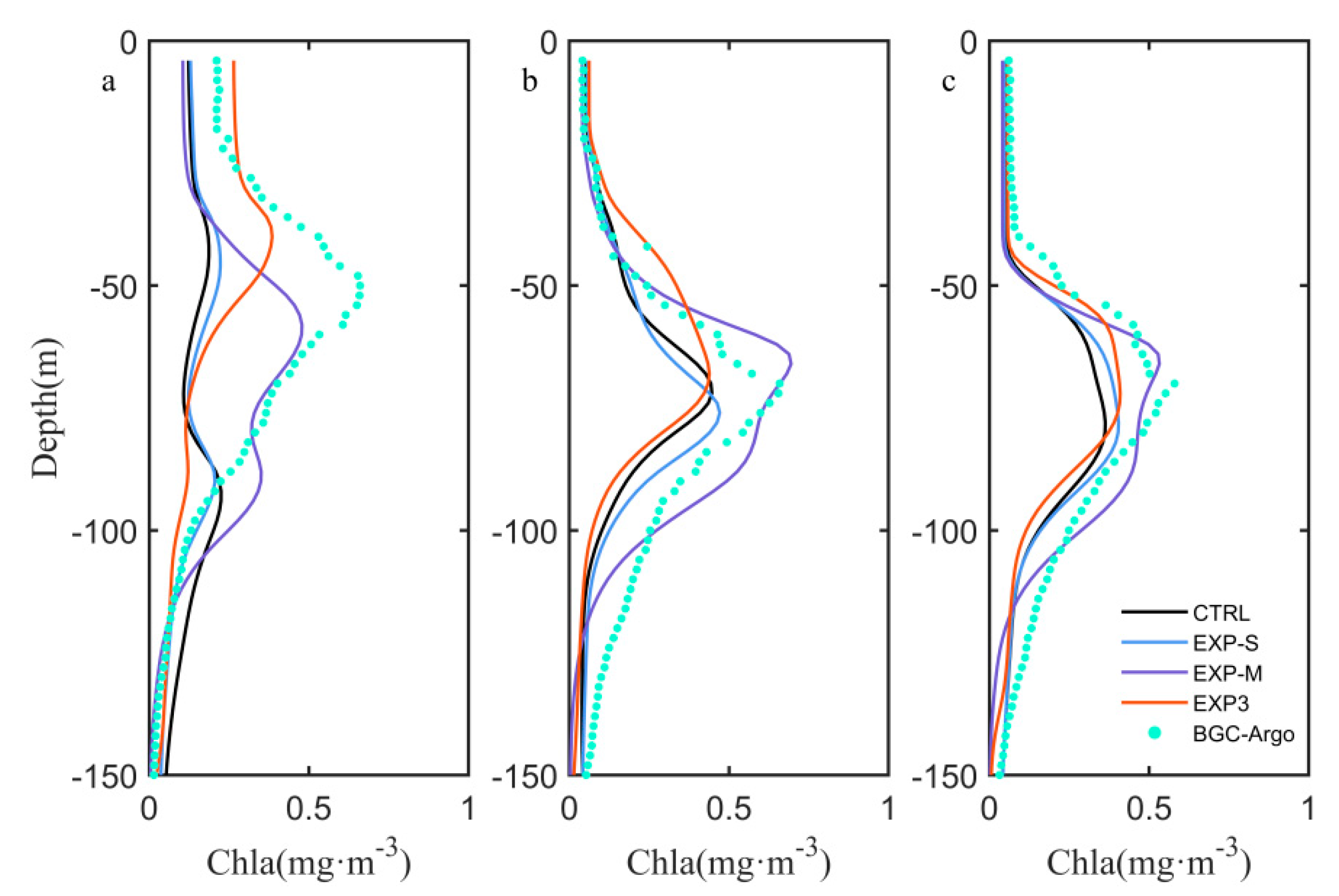
4.1. Influence of Sampling Frequency of Float Data

With respect to the traditional sampling from ship cruises, the advantage of BGC-Argo float is sampling the ocean continuously and with a relatively high frequency, returning vertical profiles associated with different spatial and temporal scales. Kaufman et al. [31] demonstrated the benefit of assimilating high-frequency data in a 1D model. BGC-Argo float sampling frequency of 1~5 days has the potential to resolve intraseasonal and mesoscale processes in the northern SCS [59].
To examine the influence of the sampling frequency on the assimilation performance, we conducted two more experiments, calculating the seasonal average (EXP-S) and monthly average (EXP-M) float profiles, respectively. GA optimization settings are similar to the EXP3, only changing the calculation of the cost function. In EXP-S, the observations of cost function used chlorophyll-a profiles of four seasonal averages. After the assimilation, the vertical chlorophyll-a bias decreases by 6.9%, and the SCM bias decreases by 22.7% with respect to the CTRL (Table 4). However, the misfit of seasonal mean chlorophyll-a profiles between the model and the float data shows less reduction (Figure 8), which may result from the fact that the four seasonal chlorophyll-a profiles are not enough to model optimization. In the EXP-M, monthly mean chlorophyll-a profiles were computed from the float data and used in the optimization. The result indicates that the SCM bias yields the largest reduction and each item of cost function and shows considerable improvements compared to the CTRL model. The depth and magnitude of SCM show the consistency with the observed data well (Figure 8), indicating that using monthly mean profiles is sufficient to contribute to the optimization of vertical chlorophyll-a structure and maintain the optimal calibration of the biological parameters. This was also found in Bisson et al. [62]. EXP-M improves the vertical chlorophyll-a even more than EXP3, probably indicting that high-frequency variabilities associated with the float data of every 1~5 days are not fully represented in the model, and assimilating those variabilities into the 1D model may increase the model-data deviations. It is particularly clear in March. In the northern SCS, March is a transition season between summer and winter monsoons, when the seasonal influence on the vertical distribution of chlorophyll-a is not the dominant factor. Instead, local processes and/or mesoscale processes may affect phytoplankton distributions measured by the BGC-Argo float, which are not resolved by the 1D model. As the dominant variability of phytoplankton in the northern SCS is at the seasonal timescale, monthly float data are more suitable to apply to the data assimilation for the 1D model.

4.2. Effects of Biological Parameter on Vertical Chlorophyll-a Structure

In the experiments above, the main differences in the vertical Chla simulation are the magnitude and the depth of SCM layer. The depth and magnitude of SCM layer largely depend on the phytoplankton dynamics, which are influenced by biological parameters. Among the optimization parameters, gmaxs1, amaxs1, and akno3s2 are related to phytoplankton growth. Beta1, beta2, akz2, and bgamma1 are related to zooplankton growth and grazing processes. The assimilation of vertical float observations significantly improves subsurface predictions of chlorophyll-a in EXP2, EXP3, and EXP-M. The EXP-M shows the best prediction skill in vertical chlorophyll-a structure, which is consistent with the BGC-Argo profile.
The optimal parameter values of each experiment are shown in Table 5. In EXP2 and EXP3, biological parameters show similar variation in value compared with CTRL model, but the magnitude of SCM in EXP3 is slightly smaller than that in EXP2 (Figure 7), which might be due to the change of gmaxs1, amaxs1, and akno3s2. Based on Michaelis–Menten equation, the decrease of the maximum specific growth rate in EXP3 will weaken the phytoplankton growth rate. The amaxs1 shows the ability of pico-phytoplankton to utilize solar irradiance for photosynthesis. EXP3 model with a smaller amaxs1 suggests a slightly weaker photosynthesis ability of pico-phytoplankton. Nitrogen limitation plays an important role in modulating the phytoplankton growth in the deep basin of the SCS [49]. Parameter akno3s2 represents the half-saturation of nitrate uptake by diatom. Thus, EXP3 with a smaller akno3s2 will improve the growth of diatom and increase sea surface chlorophyll-a concentration of diatom. Besides, EXP3 has a slightly shallower SCM layer than EXP2 because of the enhancement of zooplankton grazing processes. The parameters related to grazing rate and efficiency (beta1, beta2, and bgamma1) in EXP3 are higher than those in EXP2, which increase the zooplankton grazing and thus decrease the phytoplankton biomass in the upper layer in EXP3. In EXP1b, the model with a large amaxs1 value and small grazing rate also show a deeper SCM layer. The high grazing parameter values may lead to reduced phytoplankton peak and shallower SCM depth [66].
Compared to EXP2 and EXP3, ecosystem model of EXP-M has the largest gmaxs1 and amaxs1, and has the smallest beta1, beta2, and bgamma1. These parameters facilitate the photosynthetic efficiency of pico-phytoplankton and reduce the zooplankton grazing rate to promote the biomass of phytoplankton. Pico-phytoplankton provides the dominant contribution of chlorophyll-a in the SCS. Parameter optimization greatly increases the biomass of pico-phytoplankton and provides better chlorophyll-a simulation results. The EXP-M also has a small akno3s2 value, leading to high growth potential of the diatom. In contrast, EXP-M has a relatively smaller akz2, which changes the grazing pressure of mesozooplankton and has the potential to change phytoplankton biomass to some extent. That is to say, ecosystem models with high nonlinearity can result in parameters that have a synergistic regulation effect on the modeled vertical chlorophyll-a structure.
The vertical chlorophyll-a structure is closely related to the process of phytoplankton growth and zooplankton grazing. Thus, relevant biological parameters can affect the depth and magnitude of the SCM. Among these parameters, the phytoplankton growth parameters tend to change the magnitude of SCM; the zooplankton grazing parameters tend to change both the magnitude and the depth of SCM. All biological parameters have nonlinear effects on the modeled vertical chlorophyll-a structure.

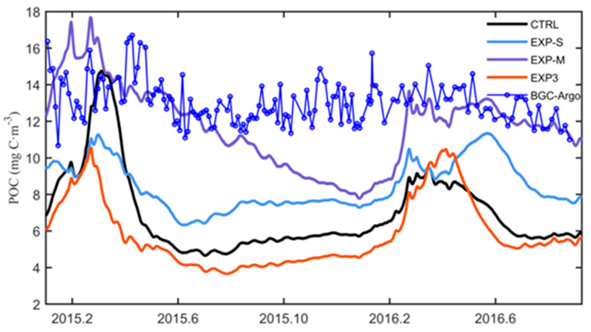
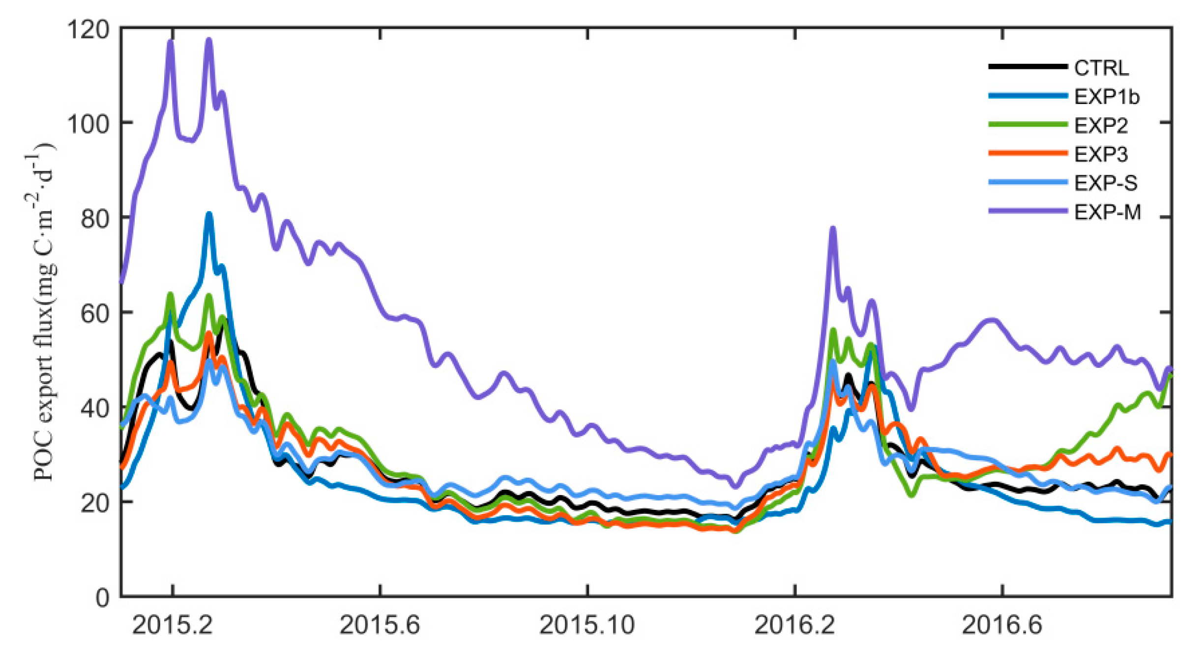
4.3. Impacts on Subsurface POC and Export Flux

Chlorophyll-a is the commonly used variable to study marine biogeochemistry. Besides, the POC is an important carbon pool that represents the biological pump transporting CO2 from the atmosphere to the ocean interior [67]. In this study, observed POC were derived from the validated bbp(700) based on the empirical relationship. Compared to other experiments, POC at 100 m depth increases significantly in the EXP-M model, which is statistically consistent with the observed data, especially in winter and spring (Figure 9). Modeled POC concentration at 100 m is comparable with previous observations at the SEATS station with a range of 1–2 mmol C m−3 [68]. In the model, the key parameters regulate the sinking pathway of POC by controlling the biological processes of phytoplankton and zooplankton. Parameter optimization improves the phytoplankton composition and adjusts the zooplankton growing and grazing process, reflecting a change of detritus concentration. Since the model predictions fit well with observations in the vertical chlorophyll-a structure, POC concentration at 100 m in the EXP-M model is largely improved compared to the CTRL model.
Marine organisms are components and also producers of POC. They produce detritus through feeding and metabolic processes that ultimately cause POC to sink downward. During in situ measurements, POC includes all the particulate (defined by the pore size of filter) organic carbon in the water column. In the model, POC concentration was calculated as the sum of phytoplankton biomass, zooplankton biomass, and detritus. Thus, uncertainties in modeled POC are generally larger than modeled individual variable, such as chlorophyll-a concentration, because more biogeochemical dynamics are involved in the POC simulation. Compared with chlorophyll-a simulation, modeled POC in EXP-M shows relatively larger bias, especially in summer and fall when surface production is considerably low in the SCS. In winter, when surface production is high, modeled POC compares well with observations. This seasonal variability is consistent with the measured POC export flux shown in previous studies. Zhou et al. [69] showed that POC export is high in winter but low during summer and fall at SEATS. Moreover, they found the correlation between surface chlorophyll-a and POC export at 100 m was significant only when Chla > 0.11 mg m−3. It indicates that other factors (phytoplankton composition, zooplankton, etc.) may play an important role in POC generation and export during the low-production period, which remains largely unknown and requires further investigations.
Carbon export flux is estimated by detritus and phytoplankton sinking in the model. The comparison of POC export flux at 100 m depth is shown in Figure 10. In EXP-M, chlorophyll-a concentrations fit the best with the BGC-Argo observations both at the SCM layer and 100 m depth. More carbon is exported from the euphotic zone due to the improvement of vertical profile of chlorophyll-a. Winter peak could reach about 110 mg C m−2 d−1 and other seasons show a low value of about 40 mg C m−2 d−1, similar to carbon export flux of the sediment trap data in the central SCS [34]. Other experiments demonstrate an underestimation of carbon export flux. Carbon export is affected by phytoplankton composition, zooplankton, and other components of the food web [70]. Phytoplankton and zooplankton communities play a significant role in controlling POC export flux [71]. Siegel et al. [72] found phytoplankton’s contribution to total export flux was on average 12.7% and a portion of the export was controlled by fecal matter from zooplankton grazing. The PFT data assimilation improves the plankton groups and results in a better prediction of carbon export flux. Therefore, it is important to improve the understanding of biogeochemical processes and food web dynamics in order to better predict POC export in the northern SCS.

5. Summary and Conclusions

Parameter optimization of marine ecosystem models provides a convenient technique for adjusting model parameters to better represent the marine ecosystem [73,74,75,76]. In this research, we implemented a genetic algorithm to optimize nine biological parameters in the CoSiNE marine ecosystem model using satellite data and BGC-Argo float observations. The application of remote sensing data improves the predictive capability of the model. The satellite-derived PFT data allow us to better simulate phytoplankton community structure, which has been used in the North Atlantic, Mediterranean Sea and global ocean. Our experiments confirmed that it could also significantly improve the model simulation in the northern SCS. However, this advantage relies on the accuracy of the PFT data. The PFT three-component model still needs more in-situ measurements to validate and evaluate in the SCS. Our study is just a preliminary application of the PFT data in the ecosystem, modeling in the SCS. Utilizing the multiplatform observational data decreases the model bias in predictions of surface and vertical chlorophyll-a distributions. All model experiments show different degrees of improvement in model skill compared with the CTRL model. After the assimilation of the satellite-derived fields, the model-predicted surface chlorophyll-a concentrations for two phytoplankton groups fit the observed values quite well, with a bias reduction of 26.8% and 49.2%, respectively. The assimilation of BGC-Argo float observations reduces the misfit of vertical chlorophyll-a profiles ranging from 11.7% to 20.3%, and the SCM bias decreases ranging from 4.7% to 32.1%.
From the experiments, data assimilation improves the simulation of the ecosystem model using both satellite PFT data and BGC-Argo observations. We show that the monthly float data are most suitable to apply in the 1D model vertical structure optimization. Parameter optimization provides better chlorophyll-a simulation by adjusting fractions of phytoplankton groups. Monthly BGC-Argo data assimilation also improves the modeled subsurface POC and POC export flux simulation by modulating the phytoplankton functional types, phytoplankton growth, and zooplankton grazing processes.
BGC-Argo floats are expanding in the global ocean, providing more opportunities and challenges for modeling, understanding, and predicting marine ecosystems. The combination of BGC-Argo observations and satellite-derived phytoplankton functional type data provides reliable support for the optimization of the model. As the 3D model requires more computational time and costs, it is difficult to optimize the parameters of 3D model directly. The success of applying the genetic algorithm in the 1D marine ecosystem model provides the basis for further application in 3D ecosystem models.

Author Contributions

Conceptualization, C.S. and P.X.; methodology, P.X. and W.M.; resources, X.X., G.Q. and S.C.; writing—original draft preparation, C.S. and P.X.; writing—review and editing, P.X. and R.J.W.B. All authors have read and agreed to the published version of the manuscript.

Funding

This study was supported by the National Natural Science Foundation of China (41890805, 41730536) and the Key Special Project for Introduced Talents Team of Southern Marine Science and Engineering Guangdong Laboratory (Guangzhou) (GML2019ZD0305). R.J.W.B was supported by the European Space Agency (ESA) project “Biological Pump and Carbon Exchange Processes (BICEP)” and a UKRI Future Leader Fellowship (MR/V022792/1). S.C. was supported by the Natural Environment Research Council (NERC) NCEO and by the NERC CAMPUS project, as well as by the SEAMLESS project, which received funding from the European Union’s Horizon 2020 research and innovation programme under grant agreement No 101004032.

Data Availability Statement

The data presented in this study are available on request from the corresponding author.

Conflicts of Interest

The authors declare no conflict of interest.

Appendix A

The term BIO(C) represents biological sources and sinks of a particular state variable. The details are as follows:
S 1 t = N P S 1 + R P S 1 G r a S 1 Z 1 M o r t S 1 A g g S 1 w 1 × S 1 z ,  
S 2 t = N P S 2 + R P S 2 G r a S 2 Z 2 M o r t S 2 A g g S 2 w 2 × S 2 z ,
C h l 1 t = N P C h l 1 G r a C h l 1 Z 1 M o r t C h l 1 A g g C h l 1 w 1 × C h l 1 z ,
C h l 2 t = N P C h l 2 G r a C h l 2 Z 2 M o r t C h l 2 A g g C h l 2 w 2 × C h l 2 z ,
Z 1 t = γ 1 × G r a S 1 Z 1 G r a Z 1 Z 2 r e g 1 × Z 1 γ 1 × r e g 1 × E x c r Z 1 ,
Z 2 t = γ 2 × ( G r a S 2 Z 2 + G r a Z 1 Z 2 + G r a S P O N Z 2 + G r a L P O N Z 2 ) M o r t Z 2 r e g 2 × Z 2 γ 2 × r e g 2 × E x c r Z 2 ,
N O 3 t = N P S 1 N P S 2 + γ 3 × N H 4 ,
N H 4 t = R P S 1 R P S 2 + r e g 1 × Z 1 + r e g 2 × Z 2 + R e m i n P O N                                               + γ 1 × r e g 1 × E x c r Z 1 + γ 2 × r e g 2 × E x c r Z 2 γ 3 × N H 4 ,
P O 4 t = ( N P S 1 N P S 2 + r e g 1 × Z 1 + r e g 2 × Z 2 + R e m i n S P O N + R e m i n L P O N ) × P 2 N ,
S i ( O H ) 4 t = ( N P S 2 R P S 2 ) × S i 2 N + R e m i n b S i ,
S P O N t = ( 1 γ 1 ) × G r a S 1 Z 1 + M o r t S 1 + A g g S 1 G r a S P O N Z 2 R e m i n S P O N w S P O N × S P O N z ,
L P O N t = ( 1 γ 2 ) × ( G r a S 2 Z 2 + G r a Z 1 Z 2 ) + M o r t S 2 + M o r t Z 2 + A g g S 2 G r a L P O N Z 2 R e m i n L P O N w L P O N × L P O N z ,
b S i t = ( G r a S 2 Z 2 + M o r t S 2 + A g g S 2 ) × S i 2 N R e m i n b S i w b S i × b S i z ,
D O t = ( N P S 1 + N P S 2 ) × O 2 N O 3 + ( R P S 1 + R P S 2 ) × O 2 N H 4 2 γ 3 × N H 4 ( r e g 1 × Z 1 + r e g 2 × Z 2 + R e m i n P O N ) × O 2 N H 4 ,
D I C t = ( N P S 1 + N P S 2 + R P S 1 + R P S 2 ) × C 2 N + ( r e g 1 × Z 1 + r e g 2 × Z 2 + R e m i n S P O N + R e m i n L P O N ) × C 2 N ,
T A L K t = N O 3 t + N H 4 t ,
where w 1 ,     w 2 , w S P O N , w L P O N , and w b S i are the sinking speed of the S1, S2, SPON, LPON, and bSi, respectively. γ1 and γ2 are grazing efficiency of Z1 and Z2. The reg1 and reg2 are excretion rate to ammonium of Z1 and Z2. P2N is the relative molecular weight ratio of P and N (Similarly, Si2N=Si/N, O2NO3=O/NO3, O2NH4=O/NH4, and C2N=C/N).
NPS1 and NPS2 represent new productions of S1 and S2. RPS1 and RPS2 represent regenerated productions of S1 and S2. MortS1(Chl1), MortS2(Chl2) and MortZ2 are mortality of S1(Chl1), S2(Chl2), and Z2. AggS1(Chl1) and AggS2(Chl2) are aggregation of S1(Chl1) and S2(Chl2). GraS1Z1(GraChl1Z1) are grazing processes of Z1 on S1(Chl1). GraS2Z2 (GraChl2Z2), GraZ1Z2, GraSPONZ2, and GraLPONZ2 are grazing processes of Z2 on S2, Z1, SPON, and LPON, respectively. ExcrZ1 and ExcrZ2 are excretion processes of Z1 and Z2. ReminSPON, ReminLPON, and ReminbSi are remineralization processes of SPON, LPON and bSi, respectively.
The calculations of biological processes are as follows.
(1) The new production and regenerated productions of S1 and S2:
N P S 1 = μ 1 m a x × m i n ( N O 3 K N O 3 s 1 + N O 3 , P O 4 K P O 4 s 1 + P O 4 ) × e ψ N H 4 × ( 1 exp ( α × I μ 1 m a x ) ) × S 1 ,
R P S 1 = μ 1 m a x × N H 4 K N H 4 s 1 + N H 4 × ( 1 exp ( α × I μ 1 m a x ) ) × S 1 ,
N P S 2 = μ 2 m a x × m i n ( N O 3 K N O 3 s 2 + N O 3 , P O 4 K P O 4 s 2 + P O 4 , S i ( O H ) 4 K S i ( O H ) 4 s 2 + S i ( O H ) 4 ) × ( 1 e x p ( α × I μ 2 m a x ) ) × S 2 ,
R P S 2 = μ 2 m a x × N H 4 K N H 4 s 2 + N H 4 × ( 1 exp ( α × I μ 2 m a x ) ) × S 2 ,
I ( z , t ) = I o ( t ) × exp ( k 1 × z k 2 × z 0 ( S 1 + S 2 ) d z ) ,
where μ 1 max and μ 2 max are the maximum growth rate of S1 and S2. ψ is the NH4 inhibition parameter. K N O 3 , K N H 4 ,   K P O 4 and K S i ( O H ) 4 are the half-saturation constants for NO3, NH4, PO4 and Si(OH)4. α is the initial slop of P-I curve.
(2) The production of chlorophyll-a:
N P C h l 1 = ρ c h l 1 × ( N P S 1 S 1 + R P S 1 S 1 ) × C h l 1 ,
ρ c h l 1 = θ m a x × N P S 1 α 1 × I × C h l 1 ,
N P C h l 2 = ρ c h l 2 × ( N P S 2 S 2 + R P S 2 S 2 ) × C h l 2 ,
ρ c h l 2 = θ m a x × N P S 2 α 2 × I × C h l 2 ,
where θ max is the maximum ratio of chlorophyll-a to carbon.
(3) The mortality:
M o r t S 1 = γ s 1 × S 1 ,  
M o r t S 2 = γ s 2 × S 2 ,
M o r t C h l 1 = γ s 1 × C h l 1 ,
M o r t C h l 2 = γ s 2 × C h l 2 ,
M o r t Z 2 = γ Z 2 × Z 2 2 ,
where γ s 1 , γ s 2 and γ Z 2 are death rate of S1, S2 and Z2.
(4) The aggregation:
A g g S 1 = γ 6 × ( S 1 + S 2 ) × S 1 ,
A g g S 2 = γ 6 × ( S 1 + S 2 ) × S 2 ,
A g g C h l 1 = γ 6 × ( S 1 + S 2 ) × C h l 1 ,
A g g C h l 2 = γ 6 × ( S 1 + S 2 ) × C h l 2 ,
where γ 6 represents the aggregation rate.
(5) The grazing (subscript is predator):
G r a S 1 Z 1 = g m a x z 1 × S 1 K z 1 + S 1 × Z 1 ,
G r a S 2 Z 2 = g m a x z 2 × ρ 1 × S 2 2 K z 2 + ζ 1 + ζ 2 × Z 2 ,
G r a Z 1 Z 2 = g m a x z 2 × ρ 2 × Z 1 2 K z 2 + ζ 1 + ζ 2 × Z 2 ,
G r a C h l 1 Z 1 = G r a S 1 Z 1 × C h l 1 S 1 × Z 1 ,
G r a C h l 2 Z 2 = G r a S 2 Z 2 × C h l 2 S 2 × Z 2 ,
G r a S P O N Z 2 = g m a x z 2 × ρ 3 × S P O N 2 K z 2 + ζ 1 + ζ 2 × Z 2 ,
G r a L P O N Z 2 = g m a x z 2 × ρ 4 × L P O N 2 K z 2 + ζ 1 + ζ 2 × Z 2 ,
ξ 1 = ρ 1 × S 2 + ρ 2 × Z 1 + ρ 3 × S P O N + ρ 4 × S P O N ,
ξ 2 = ρ 1 × S 2 2 + ρ 2 × Z 1 2 + ρ 3 × L P O N 2 + ρ 4 × L P O N 2 ,
where g m a x z 1 and g m a x z 2 are the maximal grazing rates of Z1 and Z2. K z 1 and K z 2 are the half saturation constants of Z1 and Z2 grazing. ρ is grazing preference. ρ 1 , ρ 2 , ρ 3 and ρ 4 are grazing preference for S2, Z2 grazing preference for Z1, Z2 grazing preference for SPON, and Z2 grazing preference for LPON, respectively.
(6) The excretion:
E x c r Z 1 = S 1 2 K z 1 + S 1 2 × Z 1 ,
E x c r Z 2 = ( S 2 2 K z 2 + S 2 2 + Z 1 2 K z 2 + Z 1 2 ) × Z 2 ,
(7) The remineralization:
R e m i n S P O N = γ S P O N × S P O N ,
R e m i n L P O N = γ L P O N × L P O N ,
R e m i n b S i = γ b S i × b S i ,
where γ S P O N , γ L P O N and γ b S i represent the remineralization rate of SPON, LPON and bSi.

Appendix B

The PFT three-component model of phytoplankton size classes were developed by Brewin et al. [25].
Total Chla concentration ( C ) is the sum of Chla concentrations in three size classes. Here we use OC-CCI Chla concentration. Picoplankton and nanoplankton can be combined into a single class [77], and their combined Chla concentration ( C p , n ) can be expressed as:
C p , n = C p , n m [ 1 e x p ( S p , n C ) ]   ,
where C p , n m is the asymptotic maximum value for C p , n and S p , n is the initial slope. Then the Chla of microplankton ( C m ) can simply be calculated as:
C m = C C p , n   ,
The Chla of picoplankton ( C p ) can also be expressed in a similar form as a function of total chla concentration:
C p = C p m [ 1 e x p ( S p C ) ]   ,
where C p m is the asymptotic maximum value for C p and S p determines the initial slope of the curve. Then the value of Cn can be calculated as follows:
C n = C p , n C p ,
Therefore, the fractions of these size classes can be derived by the following equations:
F m = C C p , n m [ 1 e x p ( S p , n C ) ] C   ,
F n = C p , n m [ 1 e x p ( S p , n C ) ] C p m [ 1 e x p ( S p C ) ] C   ,
F p = C p m [ 1 e x p ( S p C ) ] C   ,
where the parameter values of C p , n m , C p m , S p , n and S p in the SCS are 0.9532, 0.2563, 0.9835 and 3.5346, respectively [19].

References

  1. Friedrichs, M.A.M.; Hood, R.R.; Wiggert, J.D. Ecosystem model complexity versus physical forcing: Quantification of their relative impact with assimilated Arabian Sea data. Deep Sea Res. Part II Top. Stud. Oceanogr. 2006, 53, 576–600. [Google Scholar] [CrossRef]
  2. Bisson, K.M.; Siegel, D.A.; Devries, T. How Data Set Characteristics Influence Ocean Carbon Export Models. Glob. Biogeochem. Cycles 2018, 32, 1312–1328. [Google Scholar] [CrossRef]
  3. Fennel, K.; Losch, M.; Schröter, J.; Wenzel, M. Testing a marine ecosystem model: Sensitivity analysis and parameter optimization. J. Mar. Syst. 2001, 28, 45–63. [Google Scholar] [CrossRef] [Green Version]
  4. Kuroda, H.; Kishi, M.J. A data assimilation technique applied to estimate parameters for the NEMURO marine ecosystem model. Ecol. Model. 2004, 172, 69–85. [Google Scholar] [CrossRef]
  5. Dowd, M. Estimating parameters for a stochastic dynamic marine ecological system. Environmetrics 2011, 22, 501–515. [Google Scholar] [CrossRef]
  6. Mattern, J.P.; Dowd, M.; Fennel, K. Particle filter-based data assimilation for a three-dimensional biological ocean model and satellite observations. J. Geophys. Res. Ocean. 2013, 118, 2746–2760. [Google Scholar] [CrossRef]
  7. Xiao, Y.; Friedrichs, M.A.M. The assimilation of satellite-derived data into a one-dimensional lower trophic level marine ecosystem model. J. Geophys. Res. Ocean. 2014, 119, 2691–2712. [Google Scholar] [CrossRef] [Green Version]
  8. Gharamti, M.E.; Samuelsen, A.; Bertino, L.; Simon, E.; Korosov, A.; Daewel, U. Online tuning of ocean biogeochemical model parameters using ensemble estimation techniques: Application to a one-dimensional model in the North Atlantic. J. Mar. Syst. 2017, 168, 1–16. [Google Scholar] [CrossRef]
  9. Wang, B.; Fennel, K.; Yu, L.; Gordon, C. Assessing the value of biogeochemical argo profiles versus ocean color observations for biogeochemical model optimization in the Gulf of Mexico. Biogeosciences 2020, 17, 4059–4074. [Google Scholar] [CrossRef]
  10. Xue, H.; Chai, F.; Pettigrew, N.; Xu, D.; Shi, M.; Xu, J. Kuroshio intrusion and the circulation in the South China Sea. J. Geophys. Res. Ocean. 2004, 109, C02017. [Google Scholar] [CrossRef] [Green Version]
  11. Su, J. Overview of the South China Sea circulation and its influence on the coastal physical oceanography outside the Pearl River Estuary. Cont. Shelf Res. 2004, 24, 1745–1760. [Google Scholar] [CrossRef]
  12. Liu, K.K.; Chao, S.Y.; Shaw, P.T.; Gong, G.C.; Chen, C.C.; Tang, T.Y. Monsoon-forced chlorophyll distribution and primary production in the South China Sea: Observations and a numerical study. Deep Sea Res. Part I Oceanogr. Res. Pap. 2002, 49, 1387–1412. [Google Scholar] [CrossRef]
  13. Ning, X.; Chai, F.; Xue, H.; Cai, Y.; Liu, C.; Zhu, G.; Shi, J. Physical-biological oceanographic coupling influencing phytoplankton and primary production in the South China Sea. J. Geophys. Res. Ocean 2004, 109, C10005. [Google Scholar] [CrossRef] [Green Version]
  14. Shen, S.; Leptoukh, G.G.; Acker, J.G.; Yu, Z.; Kempler, S.J. Seasonal Variations of Chlorophyll a Concentration in the Northern South China Sea. IEEE Geosci. Remote Sens. Lett. 2008, 5, 315–319. [Google Scholar] [CrossRef]
  15. Tang, S.; Liu, F.; Chen, C. Seasonal and intraseasonal variability of surface chlorophyll a concentration in the South China Sea. Aquat. Ecosyst. Health Manag. 2014, 17, 242–251. [Google Scholar] [CrossRef]
  16. Geng, B.X.; Xiu, P.; Shu, C.; Zhang, W.Z.; Chai, F.; Li, S.; Wang, D. Evaluating the roles of wind- and buoyancy flux-induced mixing on phytoplankton dynamics in the northern and central South China Sea. J. Geophys. Res. Ocean. 2019, 124, 680–702. [Google Scholar] [CrossRef]
  17. Gong, X.; Shi, J.; Gao, H. Modeling seasonal variations of subsurface chlorophyll maximum in South China Sea. J. Ocean. Univ. China 2014, 13, 561–571. [Google Scholar] [CrossRef]
  18. Wang, S.; Li, S.; Hu, J.; Geng, B. Experiments in optimizing simulations of the subsurface chlorophyll maximum in the South China Sea. J. Mar. Syst. 2016, 156, 1–15. [Google Scholar] [CrossRef]
  19. Gong, X.; Jiang, W.; Wang, L.; Gao, H.; Boss, E.; Yao, X.; Kao, S.J.; Shi, J. Analytical solution of the nitracline with the evolution of subsurface chlorophyll maximum in stratified water columns. Biogeosciences 2017, 14, 2371–2386. [Google Scholar] [CrossRef] [Green Version]
  20. Hirata, T.; Hardman-Mountford, N.J.; Brewin, R.J.W. Synoptic relationships between surface Chlorophyll-a and diagnostic pigments specific to phytoplankton functional types. Biogeosciences 2011, 8, 311–327. [Google Scholar] [CrossRef] [Green Version]
  21. Sathyendranath, S.; Aiken, J.; Alvain, S. Phytoplankton Functional Types from Space; International Ocean-Colour Coordinating Group (IOCCG): Dartmouth, NS, Canada, 2014; p. 15. [Google Scholar]
  22. Kramer, S.J.; Roesler, C.S.; Sosik, H.M. Bio-optical discrimination of diatoms from other phytoplankton in the surface ocean: Evaluation and refinement of a model for the Northwest Atlantic. Remote Sens. Environ. 2018, 217, 126–143. [Google Scholar] [CrossRef]
  23. Kramer, S.J.; Siegel, D.A. How Can Phytoplankton Pigments Be Best Used to Characterize Surface Ocean Phytoplankton Groups for Ocean Color Remote Sensing Algorithms? J. Geophys. Res. Ocean. 2019, 124, 7557–7574. [Google Scholar] [CrossRef] [PubMed]
  24. Lin, J.; Cao, W.; Wang, G.; Hu, S. Satellite-observed variability of phytoplankton size classes associated with a cold eddy in the South China Sea. Mar. Pollut. Bull. 2014, 83, 190–197. [Google Scholar] [CrossRef] [PubMed]
  25. Brewin, R.J.W.; Stefano, C.; Shubha, S.; Thomas, J.; Gavin, T.; Kieran, C.; Airs, R.L.; Denise, C.; Vanda, B.; Emanuele, O. Uncertainty in ocean-Color estimates of chlorophyll for phytoplankton groups. Front. Mar. Sci. 2017, 4, 104. [Google Scholar] [CrossRef] [Green Version]
  26. Ciavatta, S.; Brewin, R.J.W.; Skákala, J.; Polimene, L.; De Mora, L.; Artioli, Y.; Allen, J.I. Assimilation of ocean-color plankton functional types to improve marine ecosystem simulations. J. Geophys. Res. Ocean. 2018, 123, 834–854. [Google Scholar] [CrossRef] [Green Version]
  27. Skákala, J.; Ford, D.; Brewin, R.J.W.; McEwan, R.; Kay, S.; Taylor, B.; de Mora, L.; Ciavatta, S. The assimilation of phytoplankton functional types for operational forecasting in the northwest European shelf. J. Geophys. Res. Ocean. 2018, 123, 5230–5247. [Google Scholar] [CrossRef] [Green Version]
  28. Ciavatta, S.; Kay, S.; Brewin, R.J.W.; Cox, R.; Di Cicco, A.; Nencioli, F.; Polimene, L.; Sammartino, M.; Santoleri, R.; Skákala, J. Ecoregions in the Mediterranean Sea through the reanalysis of phytoplankton functional types and carbon fluxes. J. Geophys. Res. Ocean. 2019, 124, 6737–6759. [Google Scholar] [CrossRef] [Green Version]
  29. Pradhan, H.K.; Völker, C.; Losa, S.N.; Bracher, A.; Nerger, L. Global assimilation of ocean-color data of phytoplankton functional types: Impact of different data sets. J. Geophys. Res. Ocean. 2020, 125, e2019JC015586. [Google Scholar] [CrossRef] [Green Version]
  30. Hoshiba, Y.; Hirata, T.; Shigemitsu, M.; Nakano, H.; Hashioka, T.; Masuda, Y.; Yamanaka, Y. Biological data assimilation for parameter estimation of a phytoplankton functional type model for the western North Pacific. Ocean. Sci. 2018, 14, 371–386. [Google Scholar] [CrossRef]
  31. Kaufman, D.E.; Friedrichs, M.A.M.; Hemmings, J.C.P.; Smith, W.O., Jr. Assimilating bio-optical glider data during a phytoplankton bloom in the southern Ross Sea. Biogeosciences 2018, 15, 73–90. [Google Scholar] [CrossRef] [Green Version]
  32. Shchepetkin, A.F.; Mcwilliams, J.C. The regional oceanic modeling system (roms): A split-explicit, free-surface, topography-following-coordinate oceanic model. Ocean. Model. 2005, 9, 347–404. [Google Scholar] [CrossRef]
  33. Chai, F.; Dugdale, R.C.; Peng, T.H.; Wilkerson, F.P.; Barber, R.T. One-dimensional ecosystem model of the equatorial Pacific upwelling system. Part I: Model development and silicon and nitrogen cycle. Deep Sea Res. Part II Top. Stud. Oceanogr. 2002, 49, 2713–2745. [Google Scholar] [CrossRef]
  34. Ma, W.; Xiu, P.; Chai, F.; Li, H. Seasonal variability of the carbon export in the central South China Sea. Ocean. Dyn. 2019, 69, 955–966. [Google Scholar] [CrossRef]
  35. Geider, R.J.; Macintyre, H.L.; Kana, T.M. Dynamic model of phytoplankton growth and acclimation: Responses of the balanced growth rate and the chlorophyll a:carbon ratio to light, nutrient-limitation and temperature. Mar. Ecol. Prog. Ser. 1997, 148, 187–200. [Google Scholar] [CrossRef] [Green Version]
  36. Xiu, P.; Chai, F. Modeled biogeochemical responses to mesoscale eddies in the South China Sea. J. Geophys. Res. Ocean. 2011, 116, C10006. [Google Scholar] [CrossRef] [Green Version]
  37. Guo, L.; Xiu, P.; Chai, F.; Xue, H.; Wang, D.; Sun, J. Enhanced chlorophyll concentrations induced by Kuroshio intrusion fronts in the northern South China Sea. Geophys. Res. Lett. 2017, 44, 11565–11572. [Google Scholar] [CrossRef] [Green Version]
  38. Geng, B.X.; Xiu, P.; Liu, N.; He, X.Q.; Chai, F. Biological response to the interaction of a mesoscale eddy and the river plume in the northern South China Sea. J. Geophys. Res. Ocean. 2021, 126, e2021JC017244. [Google Scholar] [CrossRef]
  39. Shaw, P.T.; Chao, S.Y.; Liu, K.K.; Pai, S.C.; Liu, C.T. Winter upwelling off Luzon in the northeastern South China Sea. J. Geophys. Res. Ocean. 1996, 101, 16435–16448. [Google Scholar] [CrossRef]
  40. Gan, J.; Li, L.; Wang, D.; Guo, X. Interaction of a river plume with coastal upwelling in the northeastern South China Sea. Cont. Shelf Res. 2009, 29, 728–740. [Google Scholar] [CrossRef]
  41. Jing, Z.Y.; Qi, Y.Q.; Hua, Z.L.; Zhang, H. Numerical study on the summer upwelling system in the northern continental shelf of the South China Sea. Cont. Shelf Res. 2009, 29, 467–478. [Google Scholar] [CrossRef] [Green Version]
  42. Wong, G.T.F.; Tseng, C.M.; Wen, L.S.; Chung, S.W. Nutrient dynamics and N-anomaly at the SEATS station. Deep Sea Res. Part II Top. Stud. Oceanogr. 2007, 54, 1528–1545. [Google Scholar] [CrossRef]
  43. Xiu, P.; Chai, F.; Shi, L.; Xue, H.; Chao, Y. A census of eddy activities in the South China Sea during 1993-2007. J. Geophys. Res. Ocean. 2010, 115, C03012. [Google Scholar] [CrossRef] [Green Version]
  44. Evans, G.T.; Parslow, J.S. A model of annual plankton cycles. Biol. Oceanogr. 1985, 3, 327–347. [Google Scholar] [CrossRef]
  45. Fasham, M.J.R. Variations in the seasonal cycle of biological production in subarctic oceans: A model sensitivity analysis. Deep Sea Res. Part I Oceanogr. Res. Pap. 1995, 42, 1111–1149. [Google Scholar] [CrossRef]
  46. Kishi, M.J.; Kashiwai, M.; Ware, D.M.; Megrey, B.A.; Eslinger, D.L.; Werner, F.E.; Noguchi-Aita, M.; Azumaya, T.; Fujii, M.; Hashimoto, S.; et al. NEMURO—a lower trophic level model for the North Pacific marine ecosystem. Ecol. Model. 2007, 202, 12–25. [Google Scholar] [CrossRef] [Green Version]
  47. Hemmings, J.C.P.; Challenor, P.G.; Yool, A. Mechanistic site-based emulation of a global ocean biogeochemical model (MEDUSA 1.0) for parametric analysis and calibration: An application of the Marine Model Optimization Testbed (MarMOT 1.1). Geosci. Model. Dev. 2015, 8, 697–731. [Google Scholar] [CrossRef] [Green Version]
  48. Ji, X.; Liu, G.; Gao, S.; Wang, H. Parameter sensitivity study of the biogeochemical model in the China coastal seas. Acta Oceanol. Sin. 2015, 34, 51–60. [Google Scholar] [CrossRef]
  49. Sankar, S.; Polimene, L.; Marin, L.; Menon, N.N.; Ciavatta, S. Sensitivity of the simulated Oxygen Minimum Zone to biogeochemical processes at an oligotrophic site in the Arabian Sea. Ecol. Model. 2018, 372, 12–23. [Google Scholar] [CrossRef] [Green Version]
  50. Saltelli, A.; Ratto, M.; Andres, T.; Campolongo, F.; Tarantola, S. Global Sensitivity Analysis the Primer; John Wiley & Sons: Hoboken, NJ, USA, 2008. [Google Scholar]
  51. Schmitt, L.M. Fundamental study theory of genetic algorithms. Theor. Comput. Sci. 2001, 259, 1–61. [Google Scholar] [CrossRef] [Green Version]
  52. Sathyendranath, S.; Brewin, R.; Brockmann, C.; Brotas, V.; Platt, T. An Ocean-Colour Time Series for Use in Climate Studies: The Experience of the Ocean-Colour Climate Change Initiative (OC-CCI). Sensors 2019, 19, 4285. [Google Scholar] [CrossRef] [Green Version]
  53. Boss, E.; Swift, D.; Taylor, L.; Brickley, P.; Zaneveld, R.; Riser, S.; Perry, M.J.; Strutton, P.G. Observations of pigment and particle distributions in the western North Atlantic from an autonomous float and ocean color satellite. Limnol. Oceanogr. 2008, 53, 2112–2122. [Google Scholar] [CrossRef] [Green Version]
  54. Cullen, J.J. The deep chlorophyll maximum: Comparing vertical profiles of chlorophyll a. Can. J. Fish. Aquat. Sci. 1982, 39, 791–803. [Google Scholar] [CrossRef]
  55. Xing, X.; Qiu, G.; Boss, E.; Wang, H. Temporal and vertical variations of particulate and dissolved optical properties in the South China Sea. J. Geophys. Res. Ocean. 2019, 124, 3779–3795. [Google Scholar] [CrossRef] [Green Version]
  56. Bisson, K.M.; Boss, E.; Westberry, T.K.; Behrenfeld, M.J. Evaluating satellite estimates of particulate backscatter in the global open ocean using autonomous profiling floats. Opt. Express 2019, 27, 30191–30203. [Google Scholar] [CrossRef] [PubMed]
  57. Haëntjens, N.; Della Penna, A.; Briggs, N.; Karp-Boss, L.; Gaube, P.; Claustre, H.; Boss, E. Detecting mesopelagic organisms using biogeochemical-Argo floats. Geophys. Res. Lett. 2020, 47, e2019GL086088. [Google Scholar] [CrossRef] [PubMed] [Green Version]
  58. Stramski, D.; Reynolds, R.A.; Babin, M.; Kaczmarek, S.; Lewis, M.R.; Röttgers, R.; Sciandra, A.; Stramska, M.; Twardowski, M.S.; Franz, B.A.; et al. Relationships between the surface concentration of particulate organic carbon and optical properties in the eastern South Pacific and eastern Atlantic Oceans. Biogeosciences 2008, 5, 171–201. [Google Scholar] [CrossRef] [Green Version]
  59. Qiu, G.; Xing, X.; Boss, E.S.; Yan, X.H.; Wang, H. Relationships between optical backscattering, particulate organic carbon, and phytoplankton carbon in the oligotrophic South China Sea basin. Opt. Express 2021, 29, 15159–15176. [Google Scholar] [CrossRef] [PubMed]
  60. Tseng, C.M.; Wong, G.T.F.; Lin, I.I.; Wu, C.R.; Liu, K.K. A unique seasonal pattern in phytoplankton biomass in low-latitude waters in the South China Sea. Geophys. Res. Lett. 2005, 32, L08608. [Google Scholar] [CrossRef] [Green Version]
  61. Zhang, W.Z.; Wang, H.; Chai, F.; Qiu, G. Physical drivers of chlorophyll variability in the open South China Sea. J. Geophys. Res. Ocean. 2016, 121, 7123–7140. [Google Scholar] [CrossRef]
  62. Bisson, K.M.; Boss, E.; Werdell, P.J. Seasonal bias in global ocean color observations. Appl. Opt. 2021, 60, 6978–6988. [Google Scholar] [CrossRef]
  63. Park, M.-S.; Lee, S.; Ahn, J.-H.; Lee, S.-J.; Choi, J.-K.; Ryu, J.-H. Decadal Measurements of the First Geostationary Ocean Color Satellite (GOCI) Compared with MODIS and VIIRS Data. Remote Sens. 2022, 14, 72. [Google Scholar] [CrossRef]
  64. Chen, Y.L.; Chen, H.-Y.; Karl, D.M.; Takahashi, M. Nitrogen modulates phytoplankton growth in spring in the South China Sea. Cont. Shelf Res. 2004, 24, 527–541. [Google Scholar] [CrossRef]
  65. Chen, C.-C.; Shiah, F.-K.; Chung, S.-W.; Liu, K.-K. Winter phytoplankton blooms in the shallow mixed layer of the South China Sea enhanced by upwelling. J. Mar. Syst. 2006, 59, 97–110. [Google Scholar] [CrossRef]
  66. Huang, B.; Hu, J.; Xu, H.; Cao, Z.; Wang, D. Phytoplankton community at warm eddies in the northern South China Sea in winter 2003/2004. Deep Sea Res. Part II Top. Stud. Oceanogr. 2010, 57, 1792–1798. [Google Scholar] [CrossRef]
  67. Beckmann, A.; Hense, I. Beneath the surface: Characteristics of oceanic ecosystems under weak mixing conditions—A theoretical investigation. Prog. Oceanogr. 2007, 75, 771–796. [Google Scholar] [CrossRef]
  68. De La Rocha, C.L. The Biological Pump. In Treatise on Geochemistry; Elsevier: Oxford, UK, 2007; pp. 1–29. [Google Scholar]
  69. Zhou, K.; Dai, M.; Maiti, K.; Chen, W.; Xie, Y. Impact of physical and biogeochemical forcing on particle export in the South China Sea. Prog. Oceanogr. 2020, 187, 102403. [Google Scholar] [CrossRef]
  70. Cai, P.; Zhao, D.; Wang, L.; Huang, B.; Dai, M. Role of particle stock and phytoplankton community structure in regulating particulate organic carbon export in a large marginal sea. J. Geophys. Res. Ocean. 2015, 120, 2063–2095. [Google Scholar] [CrossRef]
  71. Mouw, C.B.; Barnett, A.; McKinley, G.A.; Gloege, L.; Pilcher, D. Phytoplankton size impact on export flux in the global ocean. Glob. Biogeochem. Cycles 2016, 30, 1542–1562. [Google Scholar] [CrossRef] [Green Version]
  72. Siegel, D.A.; Buesseler, K.O.; Doney, S.C.; Sailley, S.F.; Behrenfeld, M.J.; Boyd, P.W. Global assessment of ocean carbon export by combining satellite observations and food-web models. Glob. Biogeochem. Cycles 2014, 28, 181–196. [Google Scholar] [CrossRef]
  73. Garcia-Gorriz, E.; Hoepffner, N.; Ouberdous, M. Assimilation of SeaWiFS data in a coupled physical–biological model of the Adriatic Sea. J. Mar. Syst. 2003, 40, 233–252. [Google Scholar] [CrossRef]
  74. Tjiputra, J.F.; Polzin, D.; Winguth, A.M.E. Assimilation of seasonal chlorophyll and nutrient data into an adjoint three-dimensional ocean carbon cycle model: Sensitivity analysis and ecosystem parameter optimization. Glob. Biogeochem. Cycles 2007, 21, 1–13. [Google Scholar] [CrossRef] [Green Version]
  75. Fan, W.; Lv, X. Data assimilation in a simple marine ecosystem model based on spatial biological parameterizations. Ecol. Model. 2009, 220, 1997–2008. [Google Scholar] [CrossRef]
  76. Xiao, Y.; Friedrichs, M.A.M. Using biogeochemical data assimilation to assess the relative skill of multiple ecosystem models in the Mid-Atlantic Bight: Effects of increasing the complexity of the planktonic food web. Biogeosciences 2014, 11, 3015–3030. [Google Scholar] [CrossRef] [Green Version]
  77. Brewin, R.J.W.; Sathyendranath, S.; Hirata, T.; Lavender, S.J.; Barciela, R.M.; HardmanMountford, N.J. A three-component model of phytoplankton size class for the Atlantic Ocean. Ecol. Model. 2010, 221, 1472–1483. [Google Scholar] [CrossRef]
Figure 1. Spatial distribution of surface chlorophyll-a concentration (mg m−3) in winter in the northern SCS. The background color shows the climatological Chla averaged in winter from 1998 to 2010. The white curve is the isobath of 200 m and 2000 m, respectively. The yellow pentacle shows the position of SEATS station. The red point shows the starting point of the float, and the gray curve shows the trajectory of the float.
Remotesensing 14 01297 g001
Figure 2. Flow chart of parameter optimization.
Remotesensing 14 01297 g002
Figure 3. (a) Time series of satellite-derived chlorophyll-a concentration (mg m−3) at the SEATS station. (b) Time series of BGC-Argo measured chlorophyll-a profiles (mg m−3).
Remotesensing 14 01297 g003
Figure 4. Comparison of sea surface chlorophyll-a concentration (mg m−3) from different model experiments in the optimization period.
Remotesensing 14 01297 g004
Figure 5. Comparison of chlorophyll-a concentrations (mg m−3) of pico-phytoplankton ((a) Chl1) and diatom ((b) Chl2) in the optimization period.
Remotesensing 14 01297 g005
Figure 6. Comparison of the vertical distribution of chlorophyll-a concentration (mg m−3) on 6 May 2015. Colored solid lines represent different experiments (CTRL, EXP1b, EXP2, and EXP3). Dotted lines represent the BGC-Argo observation.
Remotesensing 14 01297 g006
Figure 7. Comparison of vertical monthly chlorophyll-a concentrations averaged in March (a), June (b), and November (c) 2015. Colored solid lines represent different experiments (CTRL, EXP1b, EXP2, and EXP3). Dotted lines represent the BGC-Argo observation.
Remotesensing 14 01297 g007
Figure 8. Comparison of vertical monthly chlorophyll-a concentrations averaged in March (a), June (b), and November (c) 2015. Colored solid lines represent different experiments (CTRL, EXP-S, EXP-M and EXP3). Dotted lines represent the BGC-Argo observation.
Remotesensing 14 01297 g008
Figure 9. Comparison of modeled and measured POC concentrations (mg C m−3) at 100 m depth. Colored solid lines represent different experiments (CTRL, EXP-S, EXP-M, and EXP3). Blue dotted lines represent the BGC-Argo observation.
Remotesensing 14 01297 g009
Figure 10. Comparison of modeled POC export fluxes (mg C m−2d−1) from different model experiments at 100 m depth. Colored solid lines represent different experiments (CTRL, EXP 1b, EXP2, EXP3, EXP-S, EXP-M).
Remotesensing 14 01297 g010
Table 1. Observation data to calculate the cost function in each experiment.
ExperimentObservation Data
CTRL -
EXP1asatellite sea surface chlorophyll-a
EXP1bsatellite-derived PFT data
EXP2BGC-Argo profiles of chlorophyll-a
EXP3PFT data and BGC-Argo profiles of chlorophyll-a
EXP-SPFT data and seasonal averaged BGC-Argo profiles of chlorophyll-a
EXP-MPFT data and monthly averaged BGC-Argo profiles of chlorophyll-a
Table 2. Parameters selected for the optimization.
ParameterDescriptionInitial ValueMinimumMaximumUnitr2
reg1Z1 excretion rate to ammonium0.10.050.2day−10.083
gmaxs1maximum specific growth rate of S12.01.04.0day−10.018
beta1Z1 maximum grazing rate0.80.41.0day−10.099
beta2Z2 maximum grazing rate0.40.20.8day−10.047
akz2half saturation for Z2 grazing0.250.1250.5mmol N m−30.025
amaxs1initial slope of P-I curve of S10.0250.01250.05(W m−2 day)−10.075
akno3s2half saturation of nitrate uptake by S22.01.04.0mmol N m−30.046
bgamma1grazing efficiency of Z10.750.3751.0day−10.139
Chl2cs2_mmaximum chlorophyll-a to carbon ratio for S20.0650.030.08mg Chla (mg C)−10.056
Note: parameter initial values refer to Ma et al. [34].
Table 3. Item of cost function (unitless).
ItemFs1Fs2FvFscm
CTRL0.19450.03333.25830.0542
EXP1a0.17820.02933.58460.0477
EXP1b0.14240.01693.37840.0516
EXP20.20200.02792.59390.0368
EXP30.16000.01552.87630.0404
Note: Fs1 and Fs2 represent sea surface Chla misfit of two PFTs, pico-phytoplankton and diatom, respectively; Fv represents the vertical misfit between float and model; Fscm represents the Chla misfit between 65 m and 85 m depth.
Table 4. Item of the cost function.
ItemFvFscmFv-sFv-m
CTRL 3.25830.05421.05830.9097
EXP-S3.03480.04190.98120.8065
EXP-M2.62640.02920.74380.5916
EXP32.87630.04040.58260.6877
Note: Fv and Fscm are the same as those in Table 3; Fv-s and Fv-m represent the vertical misfit of average seasonal Chla and monthly average Chla, respectively.
Table 5. Optimal parameter values of each experiment.
Parameterreg1gmaxs1beta1beta2akz2amaxs1akno3s2bgamma1Chl2cs2_m
CTRL0.12.00.80.40.250.0252.00.750.065
EXP1a0.0962.4120.5730.6050.4360.0241.5360.5390.041
EXP1b0.1243.0270.5180.4230.3950.0161.3710.9120.045
EXP20.1182.3030.6790.6490.3840.0261.6470.8210.057
EXP30.121.9140.7020.6720.3720.0211.3720.8740.056
EXP-S0.1511.9370.9160.4050.4140.0272.5870.8760.05
EXP-M0.0923.4710.6240.4680.3050.0481.050.7430.03
Publisher’s Note: MDPI stays neutral with regard to jurisdictional claims in published maps and institutional affiliations.

